Article

An Interactive Data-Driven (Dynamic) Multiple Attribute Decision Making Model via Interval Type-2 Fuzzy Functions

by
Adil Baykasoğlu
1,* and
İlker Gölcük
2
1
Department of Industrial Engineering, Faculty of Engineering, Dokuz Eylül University, Izmir 35397, Turkey
2
Department of Industrial Engineering, İzmir Bakırçay University, Izmir 35665, Turkey
*
Author to whom correspondence should be addressed.
Mathematics 2019, 7(7), 584; https://doi.org/10.3390/math7070584
Submission received: 16 May 2019 / Revised: 26 June 2019 / Accepted: 27 June 2019 / Published: 30 June 2019
(This article belongs to the Special Issue Fuzzy Sets, Fuzzy Logic and Their Applications)

Abstract

:
A new multiple attribute decision making (MADM) model was proposed in this paper in order to cope with the temporal performance of alternatives during different time periods. Although dynamic MADM problems are enjoying a more visible position in the literature, majority of the applications deal with combining past and present data by means of aggregation operators. There is a research gap in developing data-driven methodologies to capture the patterns and trends in the historical data. In parallel with the fact that style of decision making evolving from intuition-based to data-driven, the present study proposes a new interval type-2 fuzzy (IT2F) functions model in order to predict current performance of alternatives based on the historical decision matrices. As the availability of accurate historical data with desired quality cannot always be obtained and the data usually involves imprecision and uncertainty, predictions regarding the performance of alternatives are modeled as IT2F sets. These estimated outputs are transformed into interpretable forms by utilizing the vocabulary matching procedures. Then the interactive procedures are employed to allow decision makers to modify the predicted decision matrix based on their perceptions and subjective judgments. Finally, ranking of alternatives are performed based on past and current performance scores.

Graphical Abstract

1. Introduction

Managers are continuously engaged in a process of making decisions in a rapidly changing business environment. Making right decisions is crucial in order to attain organizational goals and effective use of resources. Quality of decisions relies heavily on the information processing capabilities by considering multiple and conflicting criteria. With the dramatic increase in the availability of information obtained from diverse set of resources, decision making becomes much more complicated and difficult. Multiple attribute decision making (MADM) offers a set of sophisticated techniques to help decision makers in selecting the best alternative by considering multiple, conflicting, and incommensurate criteria.
The field of MADM is rapidly expanding with the continuing proliferation of new techniques and applications. Many state of the art methods have been proposed such as multi-attribute utility theory (MAUT) [1,2,3], analytic hierarchy process (AHP) [4], analytic network process (ANP) [5], technique for order preference by similarity to ideal solution (TOPSIS) [6], elimination and choice translating reality (ELECTRE) [7], VlseKriterijumska Optimizacija I Kompromisno Resenje technique (VIKOR) [8], and decision-making trial and evaluation laboratory (DEMATEL) [9]. Despite many successful applications of the MADM methods currently available in the literature, the salient deficiency of these methods is their incapability to handle temporal profiles of alternatives. Unfortunately, static MADM methods cannot deal with the temporal profiles of alternatives, that is, past performance scores are not taken into consideration. In order to overcome this deficiency, data-driven, and dynamic MADM methods have been developing along with diverse applications.
In the dynamic MADM, at least two-period decision making information is considered. In addition to the alternative and criteria dimensions, time is considered as a third dimension in the dynamic MADM. With the recent advances in the information technologies, data is becoming an indispensable part of the decision making practices, which forces the pace of a paradigm shift towards data-driven decision making. As ever-more data pour through the networks of organizations, collecting, and storing performance scores of alternatives with time stamps are not cumbersome procedures anymore. As the style of decision making evolving from intuition based to data-driven, the decision makers should be supported with relevant methodologies and tools to fully capitalize the available data. However, it is evident that the field of dynamic MADM is in its infancy and the current literature is far from meeting the requirements of a fully-fledged data-driven methodology.
In one of the earliest works on the dynamic MADM, Kornbluth [10] discussed the problem of time dependence of the criteria weights, and empirical laboratory findings were used for the analysis. Decision making teams were monitored for 12 sequential decisions and the time-dependent weights were analyzed based on different scenarios. Dong et al. [11] proposed a dynamic MADM method based on relative differences between the performance scores of the subsequent time-periods. In the study, disadvantages of using absolute differences were discussed and a numerical example was provided. Lou et al. [12] proposed a dynamic MADM model to evaluate and rank country risks based on historical data. The proposed model was aimed at predicting possible credit crises in advance. The proposed model was applied to the world economy development indicators data of 32 countries. The utilités additives discriminantes (UTADIS) method was used to rank country risk scores.
Despite many new developments, the literature of the dynamic MADM field is dominated by the aggregation-operator based models. Campanella and Ribeiro [13] proposed a framework for dynamic MADM where the aggregation operators were the main computation tools, and majority of the studies in the literature employ this framework. Xu and Yager [14] proposed dynamic intuitionistic fuzzy weighted averaging and uncertain dynamic intuitionistic fuzzy weighted averaging operators. According to their model, decision matrices of the past periods are aggregated into a decision matrix, and classical MADM techniques were implemented afterwards. Park et al. [15] proposed dynamic intuitionistic fuzzy weighted geometric and uncertain dynamic intuitionistic fuzzy weighted geometric operators for dynamic MADM problems. The past decision matrices were aggregated and then the VIKOR method was used to rank the alternatives. Zhou et al. [16] hybridized dynamic triangular fuzzy weighting average operators with fuzzy VIKOR method for quality improvement pilot program selection. Dynamic feedbacks of the customers were also incorporated into the proposed model. Bali et al. [17] employed dynamic intuitionistic fuzzy weighted averaging method with TOPSIS for multi-period third-party logistics provider selection problem. Chen and Li [18] proposed a new distance measure for triangular intuitionistic fuzzy sets with an application in dynamic MADM. The weighted arithmetic averaging operator for triangular intuitionistic fuzzy numbers was used to aggregate the decision matrices of the past periods. The ranking orders were obtained by using closeness coefficients. An investment decision making was used to illustrate the proposed method. Liang et al. [19] employed evidential reasoning approach to aggregate decision matrices with incomplete information. The enterprise evaluation in a technological zone was used to illustrate the model. Bali et al. [20] proposed an integrated model based on AHP and dynamic intuitionistic fuzzy weighted averaging operator under an intuitionistic fuzzy environment. The proposed model was implemented in a personnel promotion problem.
In some of the studies, the aggregation operators were not used to aggregate the decision matrices of the past periods at the very beginning. Xu [21] proposed dynamic weighted geometric aggregation operator along with an illustrative three-period investment decision making model. Rather than aggregating the decision matrices of the past periods, aggregation was conducted based on the closeness coefficients of the different periods. Zulueta et al. [22] proposed discrete time variable index by admitting bipolar values in the aggregation. A five-period supplier selection problem was used to illustrate the proposed aggregation operator. Lin et al. [23] used grey numbers and Minkowski distance in dealing with dynamic subcontractor selection problem. The proposed method calculated the period weighted distances to the ideal and anti-ideal solutions. Similar aggregation operator-based studies in the literature, which utilize intuitionistic fuzzy numbers [24,25], 2-tuple linguistic representation [26,27,28,29,30], grey numbers [31,32], etc. can be found. For more information about dynamic aggregation operators, we refer to a review paper [33]. On the other hand, non-aggregation operator based studies can be summarized as follows: Saaty [34] studied time-dependent eigenvectors and approximating functional forms of relative priorities in dynamic MADM. Hashemkhani Zolfani et al. [35] emphasized the relevance and necessity of future studies in MADM problems. In the paper, scenario-based MADM papers were reviewed and analyzed. Possible changes in the experts’ evaluations were expressed by using probabilities. Orji and Wei [36] integrated fuzzy logic and system dynamics simulation to sustainable supplier selection problem. Very recently, Baykasoğlu and Gölcük [37] proposed a dynamic MADM model by learning of fuzzy cognitive maps. In the study, fuzzy cognitive maps were trained by using a metaheuristic algorithm in order to capture patterns and trends in the past data. Then, the trained model was used to generate short-, medium-, and long-term future decision matrices. Finally, past, current and future decision matrices were used to rank the alternatives. The proposed model was realized in a real-life supplier selection problem.
Although a wide range of applications have been provided in the context of dynamic MADM, the literature still lacks the following considerations:
  • Decision makers are expected to fill out tedious questionnaires to articulate their preferences over alternatives at each period. This is especially very time consuming and demanding when the number of criteria and alternatives are high, and the decision points are frequent, i.e., performance evaluation, risk assessment, etc.
  • The models do not provide any mechanism to help decision makers making use of past decision making matrices when articulating their preferences at the current period. An interactive mechanism is needed to facilitate preference elicitation in the light of historical performance of alternatives.
Due to the availability of accurate historical data with high quality and quantity cannot always be assured and the data is usually affected by imprecision and noise, the predictions regarding the performance of alternatives should handle uncertainty properly. Interval type-2 fuzzy (IT2F) sets are very suitable tools for manipulating and reasoning with uncertain information. For that reason, the present study makes use of IT2F regression [38] to predict the current decision matrix. In order to enhance the prediction capability of the IT2F regression, a new hybrid IT2F model is proposed on the basis of highly practical method of so called “fuzzy functions” [39]. The proposed model is able to capture nonlinearities more successfully than the traditional fuzzy regression models, due to its unique and intelligent way of integrating membership grades of data points into the prediction problem.
The proposed dynamic MADM model contributes to the literature with its following features:
  • A dynamic MADM model is proposed based on a new IT2F functions approach.
  • An interactive procedure is provided that the current decision making matrix is predicted in forms of IT2F sets. Moreover, vocabulary matching procedure is developed so that the predicted performance scores of alternatives are recommended to the decision makers through linguistic terms such as low, medium, high, etc.
  • The proposed model interacts with decision makers whose subjective judgments are combined with the notion of “let the data speak for itself”. By providing decision makers with data-driven suggestions regarding the performance of alternatives, preference elicitation effort at each period is considerably reduced.
  • The proposed model does not require any technical knowledge such as fuzzy sets, t-norms, t-conorms, implication functions, etc. The proposed model can be easily integrated into the legacy systems of the firms, since the crisp values are processed when providing IT2F outputs.
  • A real-life personnel promotion problem is used to demonstrate the applicability of the proposed model. Rankings of employees are calculated based on past and current performance matrices with appropriate time series weights.
This paper is organized as follows: Theoretical background on the methodologies used within the scope of this paper is given in Section 2. The proposed model is provided in Section 3. The real life application of the proposed dynamic MADM model is illustrated in Section 4. Discussions are given in Section 5. Concluding remarks are given in Section 6.

2. Theoretical Background

2.1. Traditional Dynamic Multiple Attribute Decision Making

A dynamic MADM problem under study can be described as follows. Let A = { A 1 , A 2 , , A M } be a discrete set of M feasible alternatives and C = { C 1 , C 2 , , C N } be a finite set of all attributes. The set of all periods is denoted by t = { t 1 , t 2 , , t H } . Each alternative is evaluated in terms of N attributes and H periods. Each period is associated with weights that these time series weights are denoted by ξ ( t ) = [ ξ ( t 1 ) , ξ ( t 2 ) , , ξ ( t H ) ] T where ξ ( t H ) 0 and k = 1 H ξ ( t k ) = 1 . The weight vector of attributes are given by [ w 1 ( t k ) , w 2 ( t k ) , w N ( t k ) ] T where w i ( t k ) 0 and i = 1 N w i ( t k ) = 1 . The decision matrix at the period t k is denoted by A ( t k ) = ( a i j ( t k ) ) N × M where a i j ( t k ) is the value of alternative A j with respect to attribute C i at period t k . Let Ω b and Ω c be the set of benefit and cost attributes, respectively. Due to the immensurability of the different attributes, decision matrix A ( t k ) is normalized to corresponding dimensionless decision matrix R ( t k ) = ( r i j ( t k ) ) N × M by using the following formulas:
r i j ( t k ) = a i j ( t k ) max j { a i j ( t k ) } , j = 1 , 2 , , M ;   k = 1 , 2 , , H ;   i Ω b ,
r i j ( t k ) = min j { a i j ( t k ) } a i j ( t k ) , j = 1 , 2 , , M ;   k = 1 , 2 , , H ;   i Ω c ,
Hence, the normalized decision matrix is obtained as:
R ( t k ) = [ r 11 ( t k ) r 12 ( t k ) r 1 M ( t k ) r 21 ( t k ) r 22 ( t k ) r 2 M ( t k ) r N 1 ( t k ) r N 2 ( t k ) r N M ( t k ) ] .
The overall assessment value of the j th alternative is calculated by:
y j = k = 1 H i = 1 N ξ ( t k ) w i ( t k ) r i j ( t k ) ,   j = 1 , 2 , , M .
Therefore, alternatives are ranked based on y j in which the best alternative is with the highest overall assessment value.

2.2. Possibilistic Fuzzy Regression

In this section, possibilistic fuzzy regression analysis with asymmetric fuzzy numbers is overviewed based on [38]. Although there are a variety of fuzzy regression approaches developed during the last two decades, regression models relying on possibility and necessity concepts have pivotal role in the current literature. Possibilistic models strive to minimize sum of spreads in such a way that the estimated outputs must include the given targets. It is indeed advantageous to have asymmetric fuzzy numbers in possibilistic models as the lower and upper bounds of the estimated model are not necessarily equidistant from the center, which implies superior capability to capture central tendency. A fuzzy regression model can be formalized as:
Y ( x ) = β ˜ 0 + β ˜ 1 x 1 + + β ˜ n v x n v = β ˜ x ,
where the input vector is represented by x = ( 1 , x 1 , , x n v ) t and β ˜ = ( β ˜ 0 , β ˜ 1 , , β ˜ n v ) is a vector of fuzzy coefficients, and Y ( x ) is the estimated fuzzy output. The coefficients β ˜ i are denoted as β ˜ i = ( a i , c i , d i ) can be defined by:
μ A i ( x ) = { 1 ( a i x ) / c i , if a i c i x a i 1 ( x a i ) / d i , if a i x a i + d i 0 , otherwise ,
where a i represents center, and c i and d i left- and right-spreads, respectively.
Given the input-output data as ( x j , y j ) = ( 1 , x j , 1 , , x j , n v ; y j ) , j = 1 , 2 , , n d , where x j , n v being value of the variable n v of the j-th data-point among the total of n d data-points, the estimated output Y ( x j ) can be calculated by using fuzzy arithmetic. Representing regression coefficients as β ˜ i = ( a i , c i , d i ) , ( i = 0 , 1 , , n v ) , fuzzy regression model can be expressed as:
Y ( x j ) = ( a 0 , c 0 , d 0 ) + ( a 1 , c 1 , d 1 ) x j , 1 + + ( a n , c n , d n ) x j , n v .
Equation (7) can be written in a more compact form as given in Equation (8).
Y ( x j ) = ( θ C ( x j ) , θ L ( x j ) , θ R ( x j ) ) ,
where the terms θ C ( x j ) , θ L ( x j ) , θ R ( x j ) , are calculated as given in Equation (9).
θ C ( x j ) = i = 0 n a i x j i θ L ( x j ) = x j i 0 n c i x j i x j i < 0 n d i x j i θ R ( x j ) = x j i 0 n d i x j i x j i < 0 n c i x j i .
Finally, the possibilistic fuzzy regression model can be written as:
J = j = 1 n d ( y j a t x j ) 2 + ( 1 h ) j = 1 n d ( c t | x j | + d t | x j | ) + ξ ( c t c + d t d ) subject to θ C ( x j ) + ( 1 h ) θ R ( x j ) y j θ C ( x j ) ( 1 h ) θ L ( x j ) y j c i 0 , d i 0 , i = 0 , 1 , , n v ,
where ξ is a small positive number. The term ξ ( c t c + d t d ) is added to objective function so that the objective function becomes a quadratic function with respect to decision variables a , c , and d . The resulting optimization problem is a quadratic optimization problem, which involves minimizing a quadratic objective function subject to linear constrains. The possibilistic fuzzy regression analysis will be detailed in the subsequent sections.

2.3. Turksen’s Fuzzy Functions Approach

Turksen [39] proposed a new fuzzy modeling technique as an alternative to classical fuzzy rule bases (FRB). Fuzzy rule bases (FRB) have been effectively used as a facilitator to decision makers’ problem solving activities. FRBs are the one of the best currently available means to codify human knowledge. This knowledge is represented by “IF…THEN” rule structures. The “IF” part represents the antecedents and “THEN” part represents consequents. In the literature, there are different FRB system modeling strategies with unique antecedent and consequent parameter formation approaches. In these systems, membership values have also different interpretations such as “degree of fire”, “degree of compatibility”, “degree of belongingness”, or “weight or strength of local functions”. The fuzzy functions approach adds a new means of membership degrees to the list by exploiting the predictor power of membership grades [40].
The representation of each unique rule of an FRB system by means of fuzzy functions is the governing idea of the fuzzy functions approach. In the fuzzy functions approach, the membership degree of each sample vector directly affects the local fuzzy functions. One of the advantages of the fuzzy functions approach is that even non-experts can build fuzzy models as there are lower steps and parameters. It is quite practical to identify and reason with the fuzzy functions approach that some technical information regarding constructing fuzzy system models is not required such as fuzzification, t-norms and t-conorms, modus ponens, etc.
A vast array of fuzzy modeling approaches has been developed in the literature where the expert knowledge is encoded to define linguistic variables characterized by fuzzy sets. However, majority of the approaches suffers from a major drawback of being subjective and not generalizable. In order to reduce expert intervention into fuzzy system modeling, more objective methods have been developed [41,42,43,44,45]. In these systems, membership grades are not defined by decision makers, on the contrary, they are extracted from the dataset. There are also some approaches where some sophisticated techniques are integrated into fuzzy models so that the hybrid fuzzy system models are built. The prominent examples of these methods are neuro-fuzzy systems [46] and genetic-fuzzy systems [47].
There are still enduring challenges in the mentioned fuzzy system modeling approaches. Main disadvantages of the classical fuzzy system modeling approaches can be listed as follows:
  • Membership functions pertaining to antecedent and consequent parts of the fuzzy rules should be identified.
  • Aggregation of antecedents requires selection of suitable conjunction and disjunction operators (t-norms, t-conorms).
  • Proper implication operators should be identified for representation of the rules, which can be a challenging issue.
  • A suitable defuzzification method should be identified.
The fuzzy functions approach mainly reduces the number of fuzzy operators by taking advantage of data-driven modeling. For instance, fuzzy operators in determination of the membership functions in antecedents and consequents, fuzzification, aggregation of antecedents, implication, and in aggregation of consequents. It can be said that the fuzzy functions are more practical than their counterpart FRB models. Fuzzy function can be simply described as follows:
The training dataset is partitioned into c overlapping clusters where each cluster center is represented by v i , i = 1 , 2 , , c .
For each one of the clusters, a local fuzzy model f i : v i is built and one output is produced for each cluster. Here, memberships and their several transformations are added into the input space and the augmented input matrix is generated. Membership grades and their transformations are considered as new variables in the regression matrix. Practically, least square estimation is used to derive regression coefficients. Then, degree of belongingness of each given input vector is used to aggregate the local model outputs and the estimated values are produced.
General steps of the fuzzy functions approach can be given as:
Step 1: Matrix Z comprises of inputs and output of the system. Inputs and output of the system are clustered by using the fuzzy c-means clustering algorithm. Fuzzy c-means clustering method can be applied by using the formulas given as:
v i = j = 1 n d μ i j m z j j = 1 n d μ i j m ,   i = 1 , 2 , , c ,
μ i j = 1 h = 1 c ( v i z j v h z j ) 2 m 1 ,   i = 1 , 2 , , c ;   j = 1 , 2 , , n d ,
where . represents the Euclidean distance between data point z j to cluster center v i .
Step 2: In the second step, membership values of the input space are calculated. Here, the cluster centers identified in the previous step are used to calculate membership grades of the input data. Membership construction from the identified cluster centers is performed based on Equation (13).
μ i j = 1 h = 1 c ( v i x j v h x j ) 2 m 1 ,   i = 1 , 2 , , c ; j = 1 , 2 , , n d .
Step 3: For each cluster i , membership values of each input data sample, μ i j and original inputs are gathered together, and i-th local fuzzy function is obtained by predicting Y ( i ) = X ( i ) β ( i ) + ε ( i ) based on least squares estimation. When the number of inputs is n v , X ( i ) , and Y ( i ) matrices are as follows:
X ( i ) = [ μ i , 1 x 1 , 1 x n v , 1 μ i , 2 x 1 , 2 x n v , 2 μ i , n d x 1 , n d x n v , n d ] ,   Y ( i ) = [ y 1 y 2 y n d ] .
Step 4: Output values are calculated by aggregating the results of the local fuzzy functions as follows:
y ^ j = i = 1 c y ^ i j μ i j i = 1 c μ i j ,   j = 1 , 2 , , n d .

3. Developed IT2F Model

In this section, the developed IT2F model for dynamic MADM problems is given. First, the basics of the IT2F sets and necessary equations are overviewed. Afterwards, the IT2F regression model is revisited based on [38]. Then, the procedural steps of the proposed dynamic MADM model are given.

3.1. Interval Type-2 Fuzzy Sets

Definition 1
([48,49]). A type-2 fuzzy set A ˜ ˜ in the universe of discourse X can be represented by a type-2 membership function μ A ˜ ˜ as:
A ˜ ˜ = { ( ( x , u ) , μ A ˜ ˜ ( x , u ) ) | x X , u J x [ 0 , 1 ] , 0 μ A ˜ ˜ ( x , u ) 1 } ,
where J x denotes an interval in [0,1]. Moreover, type-2 fuzzy set A ˜ ˜ can also be represented as:
A ˜ ˜ = x X u J x μ A ˜ ˜ ( x , u ) / ( x , u ) ,
where J x [ 0 , 1 ] and denotes union over all admissible x and u .
Definition 2
([48,49]). Let A ˜ ˜ be a type-2 fuzzy set in the universe of discourse X represented by the type-2 membership function μ A ˜ ˜ . If all μ A ˜ ˜ ( x , u ) = 1 , then A ˜ ˜ is called an IT2F set. An IT2F set A ˜ ˜ , which can be regarded as a special case of a type-2 fuzzy set, is represented as follows:
A ˜ ˜ = x X u J x 1 / ( x , u ) ,
where J x [ 0 , 1 ] .
The footprint of uncertainty (FOU) is represented by the lower and upper membership functions:
F O U ( A ˜ ˜ ) = x X [ μ _ A ˜ ( x ) , μ ¯ A ˜ ( x ) ] ,
where μ _ A ˜ ( x ) and μ ¯ A ˜ ( x ) represent lower and upper membership functions, respectively.
Definition 3
([50]). An IT2F set A ˜ ˜ is said to be normal if sup μ ¯ A ˜ ( x ) = 1 and sup μ _ A ˜ ( x ) = h < 1 , where h represents the height of the lower membership function. An IT2F set A ˜ ˜ is said to be perfectly normal if sup μ ¯ A ˜ ( x ) = sup μ _ A ˜ ( x ) = 1 .
In this study, perfectly normal IT2F sets were employed so that the basic definitions and operational laws regarding perfectly normal triangular IT2F sets were overviewed.
Considering perfectly normal triangular IT2F numbers A ˜ ˜ = ( A ¯ , A _ ) = ( ( a ¯ 1 , a ¯ 2 , a ¯ 3 ; 1 ) ( a _ 1 , a _ 2 , a _ 3 ; 1 ) ) and B ˜ ˜ = ( b ¯ , b _ ) = ( ( b ¯ 1 , b ¯ 2 , b ¯ 3 ; 1 ) ( b _ 1 , b _ 2 , b _ 3 ; 1 ) ) , their operational laws are as follows [51]:
A ˜ ˜ B ˜ ˜ = ( ( a ¯ 1 + b ¯ 1 , a ¯ 2 + b ¯ 2 , a ¯ 3 + b ¯ 3 ; 1 ) , ( a _ 1 + b _ 1 , a _ 2 + b _ 2 , a _ 3 + b _ 3 ; 1 ) ) ,
A ˜ ˜ B ˜ ˜ = ( ( a ¯ 1 b ¯ 3 , a ¯ 2 b ¯ 2 , a ¯ 3 b ¯ 1 ; 1 ) , ( a _ 1 b _ 3 , a _ 2 b _ 2 , a _ 3 b _ 1 ; 1 ) ) ,
A ˜ ˜ B ˜ ˜ = ( ( a ¯ 1 × b ¯ 1 , a ¯ 2 × b ¯ 2 , a ¯ 3 × b ¯ 3 ; 1 ) , ( a _ 1 × b _ 1 , a _ 2 × b _ 2 , a _ 3 × b _ 3 ; 1 ) ) ,
A ˜ ˜ B ˜ ˜ = ( ( a ¯ 1 / b ¯ 3 , a ¯ 2 / b ¯ 2 , a ¯ 3 / b ¯ 1 ; 1 ) , ( a _ 1 / b _ 3 , a _ 2 / b _ 2 , a _ 3 / b _ 1 ; 1 ) ) ,
k × A ˜ ˜ = { ( ( k × a ¯ 1 , k × a ¯ 2 , k × a ¯ 3 ; 1 ) ( k × a _ 1 , k × a _ 2 , k × a _ 3 ; 1 ) ) , k 0 ( ( k × a ¯ 3 , k × a ¯ 2 , k × a ¯ 1 ; 1 ) ( k × a _ 3 , k × a _ 2 , k × a _ 1 ; 1 ) ) , k 0 .
Definition 4.
The ranking value R a n k ( A ˜ ˜ ) of a IT2F set A ˜ ˜ = ( A ¯ , A _ ) can be defined via the concept of centroid as [52]:
C A ˜ ˜ L = min ξ [ a , b ] a ξ x μ ¯ A ( x ) d x + ξ b x μ _ A ( x ) d x a ξ μ ¯ A ( x ) d x + ξ b μ _ A ( x ) d x ,
C A ˜ ˜ R = max ξ [ a , b ] a ξ x μ _ A ( x ) d x + ξ b x μ ¯ A ( x ) d x a ξ μ _ A ( x ) d x + ξ b μ ¯ A ( x ) d x ,
where C A ˜ ˜ L and C A ˜ ˜ R are the endpoints of the centroid. The ranking value of the IT2F set A ˜ ˜ is calculated as:
R a n k ( A ˜ ˜ ) = C A ˜ ˜ L + C A ˜ ˜ R 2 ,
where R a n k ( A ˜ ˜ ) is the centroid-based ranking value of A ˜ ˜ .
Definition 5
([53]). The Jaccard similarity measure for fuzzy sets A ˜ ˜ and B ˜ ˜ is defined by
S M ( A ˜ ˜ , B ˜ ˜ ) = X min ( μ ¯ A ( x ) , μ ¯ B ( x ) ) d x + X min ( μ _ A ( x ) , μ _ B ( x ) ) d x X max ( μ ¯ A ( x ) , μ ¯ B ( x ) ) d x + X max ( μ _ A ( x ) , μ _ B ( x ) ) d x ,
where S M represent similarity degree of fuzzy sets with respect to Jaccard measure.

3.2. IT2F Regression Model

In this section, IT2F regression model is revisited based on [38]. IT2F regression model will be utilized within the fuzzy functions approach [39] in order to increase its performance in the next section. In this section, the necessary equations are derived for IT2F regression in a step-by-step approach. IT2F regression models can be constructed based on the concepts of possibility and necessity. Here, possibility and necessity concepts are used to build an upper approximation model (UAM) and lower approximation model (LAM), respectively [54]. Building an integrated model, UAM and LAM are used to form upper and lower membership functions of the IT2F coefficients, respectively.
In mathematical terms, LAM and UAM models can be written as:
LAM : Y ˜ * ( x j ) = β ˜ * 0 + β ˜ * 1 x j 1 + + β ˜ * n x j , n v = β ˜ * x j , j = 1 , , n d UAM : Y ˜ * ( x j ) = β ˜ 0 * + β ˜ 1 * x j 1 + + β ˜ n * x j , n v = β ˜ * x j , j = 1 , , n d ,
where coefficients β ˜ * j and β ˜ j * are non-symmetric triangular fuzzy numbers. The regression coefficients β ˜ * j and β ˜ j * are shown in Figure 1.
As shown in Figure 1, β ˜ * i and β ˜ i * can be defined as:
β ˜ * i = ( b i f i , b i , b i + g i ; 1 ) β ˜ i * = ( b i f i p i , b i , b i + g i + q i ; 1 ) ,
where the condition β ˜ i * β ˜ * i , is satisfied for i = 0 , , n v .
In order to increase readability of the formulations, conventional representation of the literature is adopted here, where ( center , left _ spread , right _ spread ) is used to show the LAM and UAM as given by β ˜ * i = ( b i , f i , g i ) and β ˜ i * = ( b i , f i + p i , g i + q i ) , respectively.
The inclusion relation between β ˜ * i and β ˜ i * can be extended to Y ˜ * ( x j ) and Y ˜ * ( x j ) , that is:
Y ˜ * ( x ) Y ˜ * ( x ) for any x = ( 1 , x 1 , , x n v ) t if β ˜ i * β ˜ * i .
Using the coefficients of the LAM model A ˜ * i = ( b i , f i , g i ) , Y ˜ * ( x j ) can be expressed as:
Y ˜ * ( x j ) = ( b 0 , f 0 , g 0 ) + ( b 1 , f 1 , g 1 ) x j 1 + + ( b n v , f n v , g n v ) x j , n v = ( i = 0 n b i x j i , x j i 0 f i x j i x j i 0 g i x j i , x j i 0 g i x j i x j i 0 f i x j i , ) = ( b t x j , θ * L ( x j ) , θ * R ( x j ) ) ,
where b = ( b 0 , b 1 , , b n v ) t .
Similarly, Y ˜ * ( x j ) can be expressed as:
Y ˜ * ( x j ) = ( b 0 , f 0 , g 0 ) + ( b 1 , f 1 + p 1 , g 1 + q 1 ) x j 1 + + ( b n v , f n v + p n v , g n v + q n v ) x j n v = ( i = 0 n v b i x j i , x j i 0 f i x j i + x j i 0 p i x j i x j i 0 g i x j i x j i 0 q i x j i , x j i 0 g i x j i + x j i 0 q i x j i x j i 0 f i x j i x j i 0 p i x j i , ) = ( b t x j , θ * L ( x j ) , θ * R ( x j ) ) .
As the possibility and necessity concepts were employed, observed outputs were transformed into granular constructs by admitting a tolerance level for the left- and right-spreads. A user-defined tolerance_level was set, thereby possibilistic relationships between observed and estimated outputs could be defined. Generally, tolerance_level is a percentage type, i.e., assigning 20% of each output y j as the corresponding spread. In this study, left- and right-spreads of the observed outputs were called tolerance levels. The tolerance level for the j th data-point is denoted by e j .
The possibilistic model states that the resulting output from the UAM should cover all of the observed data-points within the given tolerance- and h-level. In other words, [ Y ˜ * ( x j ) ] h should approach to [ Y j ] h from the upper side; i.e., [ Y ˜ * ( x j ) ] h should be the least interval among all feasible solutions. This brings up the following constraints:
[ Y ˜ * ( x j ) ] h [ Y j ] h { b t x j + ( 1 h ) θ R * ( x j ) y j + ( 1 h ) e j b t x j ( 1 h ) θ L * ( x j ) y j ( 1 h ) e j } , j = 1 , , n d f 0 , g 0 , p 0 , q 0 , ,
where x j = ( 1 , x j , 1 , x j , 2 , , x j , n v ) , j = 1 , , n d and the term x j , n v denotes the value of the variable n v of the j th data point.
On the other hand, according to necessity model, the h -level set of the Y ˜ * ( x j ) should be included in the h-level set of the given output Y j . In other words, [ Y ˜ * ( x j ) ] should approach to [ Y j ] h from the lower side, i.e., [ Y ˜ * ( x j ) ] should be the greatest interval among all feasible solutions. This can be written in a constraint form as:
[ Y ˜ * ( x j ) ] h [ Y j ] h { b t x j + ( 1 h ) θ * R ( x j ) y j + ( 1 h ) e j b t x j ( 1 h ) θ * L ( x j ) y j ( 1 h ) e j } , j = 1 , , n d f 0 , g 0 ,   i = 0 , , n .
Integrating the possibility and necessity models by taking into account the inclusion relation [ Y ˜ * ( x j ) ] h [ Y ˜ * ( x j ) ] h a quadratic programming formulation of the IT2F regression model is formulated as:
min   b , f , g , p , q J = j = 1 n d ( y j b t x j ) 2 + ( 1 h ) j = 1 n d ( p t | x j | + q t | x j | ) + ξ ( f t f + g t g + p t p + q t q ) Subject   to { b t x j + ( 1 h ) θ R * ( x j ) y j + ( 1 h ) e j b t x j ( 1 h ) θ L * ( x j ) y j ( 1 h ) e j b t x j + ( 1 h ) θ * R ( x j ) y j + ( 1 h ) e j b t x j ( 1 h ) θ * L ( x j ) y j ( 1 h ) e j } f 0 , g 0 , p 0 , q 0 , j = 1 , , n d ,
where ξ is a small positive number. The term ξ ( f t f + g t g + p t p + q t q ) is inserted into the objective function so that the objective function becomes a quadratic function with respect to decision variables b , f , g , p, and q . The obtained UAM and LAM by solving the above integrated quadratic programming model always satisfy inclusion relation Y * ( x ) Y * ( x ) at the h-level.

3.3. Dynamic MADM Model via Proposed IT2F Functions

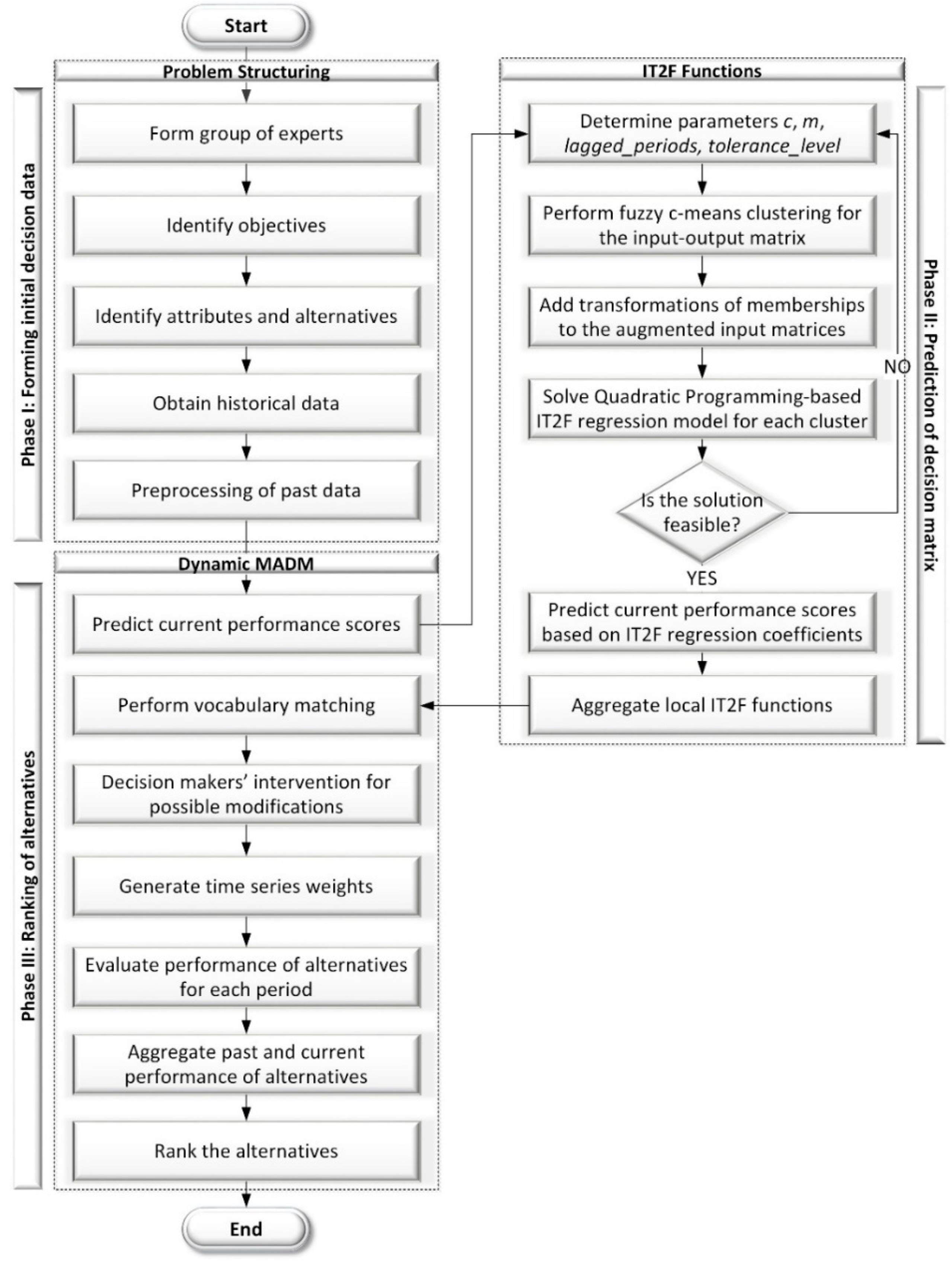
In this section, the proposed IT2F functions approach was given in a step-by-step manner. The flowchart of the proposed model is illustrated in Figure 2.

3.3.1. Phase-I: Problem Structuring

Step 1: Problem-framing: In this step, a group of experts decided on the objective of the study, and the attributes and alternatives were identified. Here, expert opinions and the literature surveys helped to arrive at problem-framing.
Step 2: Obtaining historical data: Historical records were identified and the past data were fetched from the databases. Past data contained performance values of alternatives with respect to attributes at different periods as given in Equation (37).
A ( t 1 ) = [ a 11 ( t 1 ) a 12 ( t 1 ) a 1 M ( t 1 ) a 21 ( t 1 ) a 22 ( t 1 ) a 2 M ( t 1 ) a N 1 ( t 1 ) a N 2 ( t 1 ) a N M ( t 1 ) ] , , A ( t H ) = [ a 11 ( t H ) a 12 ( t H ) a 1 M ( t H ) a 21 ( t H ) a 22 ( t H ) a 2 M ( t H ) a N 1 ( t H ) a N 2 ( t H ) a N M ( t H ) ] ,
where A ( t 1 ) and A ( t H ) are the decision matrices at the first and last period of the historical data, respectively.
This data can be unstructured so that the preprocessing is required.
Step 3: Preprocessing of historical data: In order to ensure accurate and meaningful analysis, data cleaning and preprocessing techniques are implemented in this step. Bad or missing data are eliminated by removing or replacing. Abrupt changes and local optima values are also identified. Smoothing or de-trending methods can be applied to remove noise.
Moreover, the historical decision making matrices are arranged as time series data. Here, for each alternative and attribute pair, time series data are formed. Mathematically speaking, the performance scores for a particular alternative and attribute ( a i j ( t 1 ) , a i j ( t 2 ) , , a i j ( t H ) ) are collected from each period and the time series y = ( y 1 , y 2 , , y H ) t is formed, where the number of points is equal to number of periods H .
Then, the lagged matrices are constructed where number of lagged periods is denoted by p . Note that j th data point in the input matrix x j = ( x t 1 , j , x t 2 , j , , x t p , j ) t will be used to estimate y j , j = 1 , 2 , , n d , where n d is equal to H p . The inputs and the outputs of the system are given as:
X = [ x t 1 , 1 x t 2 , 1 x t p , 1 x t 1 , 2 x t 2 , 2 x t p , 2 x t 1 , n d x t 2 , n d x t p , n d ] , Y = [ y 1 y 2 y n d ] ,
where x t p , n d represents the value of variable t p of the data point n d .
Let the number of past decision matrices are four, and the lagged periods are determined as two. Suppose that decision makers are concerned with the past performance of the second alternative with respect to the first attribute. The corresponding time series data, input and output matrices are illustrated in Table 1.

3.3.2. Phase-II: Training of Fuzzy Functions Approach

Step 4: Determining parameters of the IT2F functions model: In this step, parameters of the fuzzy c-means clustering algorithm were determined. The number of clusters c, fuzzification coefficient m, lagged_periods, and tolerance_level for calculating possibility- and necessity-based constraints in IT2F regression were defined.
Step 5: Performing fuzzy c-means clustering to input-output model: In this step, inputs and outputs of the system were used to carry out fuzzy c-means clustering. Having the inputs of the system in the form of lagged variables, the next step was to form the input–output matrix Z . The matrix Z = ( X , Y ) is composed of the input matrix X and output matrix Y . Then, elements of the Z matrix z j were clustered by using the FCM algorithm. FCM was applied by using the following formulas:
v i = k = 1 n d μ i j m z j j = 1 n d μ i j m ,   i = 1 , 2 , , c ,
μ i j = 1 h = 1 c ( v i z j v h z j ) 2 m 1 ,   i = 1 , 2 , , c ;   j = 1 , 2 , , n d ,
where . represents the Euclidian distance.
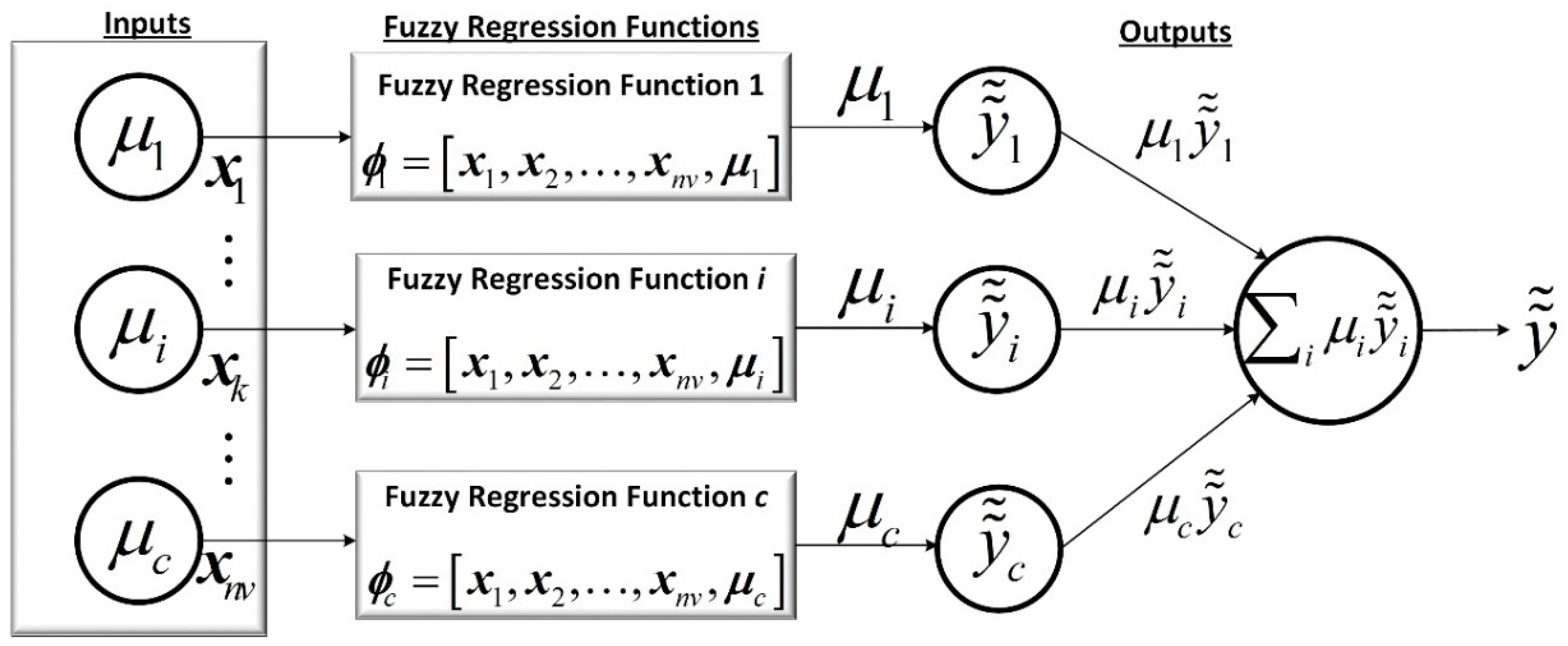
Step 6: Generating augmented input matrices: The augmented input matrix is obtained by adding memberships and their transformations into the original input matrix. Based on the cluster centers found in the Step 5, membership values of the input space are calculated as:
μ i j = 1 h = 1 c ( v i x j v h x j ) 2 m 1 ,   i = 1 , 2 , , c ;   j = 1 , 2 , , n d ,
where x denotes the input matrix.
Membership values of each input data sample, μ i j and their transformations are augmented to the original input matrix for the i th cluster as:
ϕ i = [ 1 μ i , 1 exp ( μ i , 1 ) ( μ i , 1 ) p x t 1 , 1 x t p , 1 1 1 μ i , 2 μ i , j exp ( μ i , 2 ) exp ( μ i , j ) ( μ i , 2 ) p ( μ i , j ) p x t 1 , 2 x t 1 , j x t p , 2 x t p , j 1 μ i , n d exp ( μ i , n d ) ( μ i , n d ) p x t 1 , n d x t p , n d ] ,
where j-th data point is represented by ϕ i , j = ( 1 , μ i , j , exp ( μ i , j ) , μ i , j 2 , x t 1 , j , , x t p , j ) t .
The schematic representation of the proposed IT2F functions is given in Figure 3.
Step 7: Solving quadratic programming model for each cluster: Fuzzy regression coefficients are calculated for each cluster by solving a quadratic programming model:
min   b , f , g , p , q J = j = 1 n d ( y j b t ϕ i , j ) 2 + ( 1 h ) j = 1 n d ( p t | ϕ i , j | + q t | ϕ i , j | ) + ξ ( f t f + g t g + p t p + q t q ) Subject   to { b t ϕ i , j + ( 1 h ) θ R * ( ϕ i , j ) y j + ( 1 h ) e j b t ϕ i , j ( 1 h ) θ L * ( ϕ i , j ) y j ( 1 h ) e j b t ϕ i , j + ( 1 h ) θ * R ( ϕ i , j ) y j + ( 1 h ) e j b t ϕ i , j ( 1 h ) θ * L ( ϕ i , j ) y j ( 1 h ) e j } f 0 , g 0 , p 0 , q 0 , j = 1 , , n d ,
where regression coefficients are IT2F numbers represented by β ˜ ˜ = ( ( b , f + p , g + q ) , ( b , f , g ) ) ,
Step 8: Collecting predictions of local fuzzy functions: Predicted output values are calculated as:
y ˜ ˜ i = ϕ i β ˜ ˜ i ,
where y ˜ ˜ i = ( y ˜ ˜ i , 1 , y ˜ ˜ i , 2 , , y ˜ ˜ i , j , , y ˜ ˜ i , n d ) t , β ˜ ˜ i is the regression coefficients of the ith local fuzzy function and denotes the fuzzy matrix multiplication.
Step 9: Aggregating local IT2F functions: Finally, outputs of the local fuzzy functions y ˜ ˜ i are weighted by the corresponding membership values and predicted IT2F output is calculated:
Y ˜ ˜ j = i c y ˜ ˜ i , j μ i , j i = 1 c μ i , j , j = 1 , 2 , , n d ,
where Y ˜ ˜ j is the predicted value of the j th data point.

3.3.3. Phase-III: Ranking of Alternatives

Step 10: Performing vocabulary matching: The resulting values of the IT2F functions were inherently IT2F sets. Since experts often linguistically evaluate the objects in the decision making applications and it is difficult to analytically interpret the obtained numerical values, there was a need for transforming IT2F functions results into the linguistic terms. For that aim, similarity-based vocabulary matching was implemented in this step.
Let V { V 1 , V 2 , , V U } represents the vocabulary of the linguistic terms, i.e., V U denotes the linguistic term very good, V U 1 denotes the term good, etc. The linguistic outputs of the IT2F functions approach can be given as:
A ˜ ˜ ( t C ) = [ a ˜ ˜ 11 ( t C ) a ˜ ˜ 12 ( t C ) a ˜ ˜ 1 M ( t C ) a ˜ ˜ 21 ( t C ) a ˜ ˜ 22 ( t C ) a ˜ ˜ 2 M ( t C ) a ˜ ˜ N 1 ( t C ) a ˜ ˜ N 2 ( t C ) a ˜ ˜ N M ( t C ) ] .
The a ˜ ˜ i j values are calculated as:
a ˜ ˜ i j = arg max l { 1 , 2 , , U } S M ( a ˜ ˜ i j , V l ) ,
where S M represents the Jaccard similarity measure given earlier, and V l is the l th linguistic term in the vocabulary.
Step 11: Modifying solutions if necessary: In this step, the results of IT2F functions in the form of linguistic variables were presented to the decision makers. In other words, the current decision matrix was automatically generated based on the past data. The decision makers evaluated the results and made necessary modifications if needed. The illustration of this process is given in Figure 4. Here, the decision makers’ perceptions had a pivotal role. For example, decision makers might decide on the fact that the performance of the first alternative with respect to the first and second attributes needs to be modified. Then the decision matrix takes the form as given in Equation (48).
A ˜ ˜ ( t C ) = [ a ˜ ˜ 11 ( t C ) a ˜ ˜ 12 ( t C ) a ˜ ˜ 1 M ( t C ) a ˜ ˜ 21 ( t C ) a ˜ ˜ 22 ( t C ) a ˜ ˜ 2 M ( t C ) a ˜ ˜ N 1 ( t C ) a ˜ ˜ N 2 ( t C ) a ˜ ˜ N M ( t C ) ] ,
where a ˜ ˜ i j ( t C ) represents the subjective judgments of the decision makers and a ˜ ˜ i j ( t C ) denotes the IT2F function result.
Step 12: Generating time series weights: In this step, time series weights were generated. A basic unit-interval monotonic (BUM) function was used to generate weights. Yager [55] defined the BUM function as Q : [ 0 , 1 ] [ 0 , 1 ] , where the weights are considered as quantifiers underlying the information fusion process.
  • Q ( 0 ) = 0 ,
  • Q ( 1 ) = 1 ,
  • Q ( x ) Q ( y ) , if x > y ,
    where Q ( x ) is a monotonically non-decreasing function defined in the unit interval [ 0 , 1 ] .
Based on the BUM function, the time series weights are generated as:
ξ ( t k ) = Q ( k p ) Q ( k 1 p ) ,   k = 1 , 2 , , p ,
where Q ( x ) = e α x 1 e α 1 ,   α > 0 .
According to the BUM function, the more the period is closer to the current period, the higher the weight of that period, which is a desired behavior for real-world applications.
Step 13: Evaluating performance of alternatives at each period: Performance of each alternative is calculated for different periods separately. In this step, variety of MADM methods can be employed to obtain a performance indicator. For the sake of simplicity, well-known closeness coefficient measures are used to evaluate performance of alternatives at each period. As the current decision matrix comprises of IT2F evaluations, computational steps for the IT2FSs are given in this section in order to avoid repetition. Note that the required computations for the past data are the same, except the fact that numerical values are crisp. First, the decision matrices related to past periods are normalized as given earlier in Equations (1) and (2). As the current decision matrix consists of IT2F evaluations, normalization is conducted based on the Equations (50) and (51).
r ˜ ˜ i j ( t k ) = ( ( a ¯ i j 1 ( t k ) max j { a ¯ i j 3 ( t k ) } , a ¯ i j 2 ( t k ) max j { a ¯ i j 3 ( t k ) } , a ¯ i j 3 ( t k ) max j { a ¯ i j 3 ( t k ) } ; 1 ) , ( a _ i j 1 ( t k ) max j { a ¯ i j 3 ( t k ) } , a _ i j 2 ( t k ) max j { a ¯ i j 3 ( t k ) } , a _ i j 3 ( t k ) max j { a ¯ i j 3 ( t k ) } ; 1 ) ) , if   i Ω b ,
r ˜ ˜ i j ( t k ) = ( ( min j { a ¯ i j 1 ( t k ) } a ¯ i j 3 ( t k ) , min j { a ¯ i j 1 ( t k ) } a ¯ i j 2 ( t k ) , min j { a ¯ i j 1 ( t k ) } a ¯ i j 1 ( t k ) ; 1 ) , ( min j { a ¯ i j 1 ( t k ) } a _ i j 3 ( t k ) , min j { a ¯ i j 1 ( t k ) } a _ i j 2 ( t k ) , min j { a ¯ i j 1 ( t k ) } a _ i j 1 ( t k ) ; 1 ) ) , if   i Ω c .
Then, the weighted normalized decision matrices are calculated as:
ν ˜ ˜ i j ( t k ) = r ˜ ˜ i j ( t k ) × w i ,   i = 1 , 2 , , N ,   j = 1 , 2 , , M ,   k = 1 , 2 , , H .
When the weighted normalized decision matrices are constructed, the next step is to calculate the positive ideal solutions (PIS) and negative ideal solutions (NIS) as:
PIS = ( ν 1 + , ν 2 + , , ν N + ) = { ( max j { R a n k ( ν ˜ ˜ i j ( t k ) ) } ) | i Ω b , ( min j { R a n k ( ν ˜ ˜ i j ( t k ) ) } ) | i Ω c } , k = 1 , 2 , , H
NIS = ( ν 1 , ν 2 , , ν N ) = { ( min j { R a n k ( ν ˜ ˜ i j ( t k ) ) } ) | i Ω b , ( max j { R a n k ( ν ˜ ˜ i j ( t k ) ) } ) | i Ω c } , k = 1 , 2 , , H
Then, separation measures are calculated by using the Euclidean distance as:
D j + ( t k ) = i = 1 N ( R a n k ( ν ˜ ˜ i j ( t k ) ) ν i + ( t k ) ) 2 ,
D j ( t k ) = i = 1 N ( R a n k ( ν ˜ ˜ i j ( t k ) ) ν i ( t k ) ) 2 .
Finally, closeness coefficients are calculated as:
C C j ( t k ) = D j ( t k ) ( D j + ( t k ) + D j ( t k ) ) ,
where C C j ( t k ) represents the closeness coefficient of the j th alternative at period t k .
Step 14: Aggregating past and current performance of alternatives: Finally, a dynamic weighted averaging (DWA) operator was utilized to obtain final ranking values of alternatives.
D W A ξ ( t ) ( C C j ( t 1 ) , C C j ( t 2 ) , , C C j ( t H ) ) = k = 1 H ξ ( t k ) C C j ( t k ) .
Step 15: Rank the alternatives: When the past and current performance scores of alternatives were aggregated, alternatives were ranked based on their ranking values. Higher ranking value implies superiority of an alternative.

4. Case Study

One of the most important assets of a company is undoubtedly the human resources (HRs). Regardless of how the other resources are managed in an organization, inadequacies in the management of HRs result in poor performance of many operations. Therefore, firms have steadily recognized the importance of HRs and have been taking necessary actions to increase overall performance.
Personnel promotion is a significant task in HR management that aims to select the right person for the right job. Despite its similarity with the personnel selection problem, personnel promotion problem deals with selecting appropriate personnel for higher positions within the firms’ current personnel rather than evaluating the applicants from outside the firm. Personnel promotion problem can be defined as selecting the most qualified employee among the available candidates for a vacant position by considering their performance during their employment at the firm. Hence, the personnel promotion problem is an inherently dynamic MADM problem as the temporal performance of employees are taken into consideration with respect to predetermined attributes. Unfortunately, many enterprises are not aware of the methodologies and tools to utilize historical records in their HR practices. As evaluating personnel with respect to their performance on a diverse set of criteria during their employment is cognitively demanding, firms should be supported with relevant data-driven tools.
In this study, a real-life personnel promotion problem is considered and the proposed model is implemented. The company, which was contacted within the scope of this study, was a medium sized firm involved in automobile subsidiary industry. Due to the firm policy, it was named as company A. Company A had hired three students as a part-time employee for their continuous improvement project. Upon graduation, at most two students with qualified skills will be offered to full-time job so that the supervisors have been evaluating students’ performance in a monthly basis. Therefore, performance data was used to demonstrate the procedural steps of the proposed model.

4.1. Structering Personnel Promotion Problem

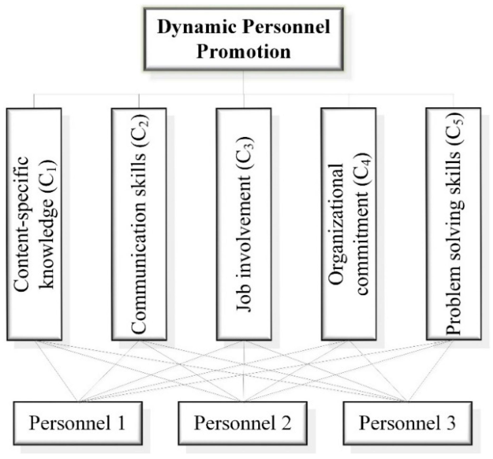
Step 1: In this step, the experts were identified based on their professional backgrounds. The heterogeneity of the experts was assured and three experts were identified. The experts were the directors of HR and production and quality control departments. After identification of the experts, participants were elucidated about the scope and details of the study. The evaluation criteria determined by the experts were employed within the scope of this study. The evaluation criteria consisted of content-specific knowledge (C1), communication skills (C2), job involvement (C3), organizational commitment (C4), and problem solving skills (C5). The decision hierarchy is given in Figure 5.
Step 2: Historical performance data of the employees with respect to predefined attributes were obtained. The company had a performance evaluation system that assigned performance scores between 0–10, 0 and 10 represented the worst and the best values, respectively. In the scope of this study, performance values of the past 1.5 years (18 months) were directly used. The historical data of the performance scores of the employee 1 with respect to decision attributes is given in Table 2. Similarly, the historical records for the employee 2 and employee 3 were obtained.
Step 3: Historical data was organized in tables, and missing values were sought for. No missing values were identified within the 18-month data period. On the other hand, it was decided not to implement normalization techniques as the proposed model could handle numeric values in the range 0–10. The historical decision matrices were also transformed into time series vectors so that the IT2F functions method could be implemented.
Afterwards, the data set was divided into training and test sets. The training set consisted of the first 80% part of the historical data and the rest of the data points were allocated to the test set.

4.2. Estimating the Current Decision Matrix

Having obtained the historical data, the next step was to employ the proposed IT2F functions approach to estimate the current decision matrix based on past data.
Step 4: In this step, parameters of the model were identified. The model parameters were the number of lagged_periods, tolerance_levels, number of cluster, and the degree of fuzzification. Instead of using cluster validity indices in order to select the optimum c and m parameters, the model parameters were selected by using a grid search for each parameter based on Root Mean Square Error (RMSE) performance metric. The tolerance_levels were set to 30% for being able to find feasible solutions for every combination of parameters when solving quadratic programming models.
The identified parameters are given in Table 3.
Step 5: In this step, the input and output matrices were combined and the FCM clustering algorithm was performed based on the parameters identified in the previous step. By utilizing FCM clustering algorithm, cluster centers were identified. These cluster centers had a key role in the Turksen’s fuzzy system model in which the clusters were used as a fuzzification engine of the classical FRB systems.
Step 6: Having identified cluster centers, the next step was to find membership grades of the input data and to form the augmented input matrices by integrating membership transformations as explanatory variables. In this study, integration of membership degrees, exponentials of the memberships, and the square of the memberships were found to exhibit good performance so that these transformations were used to augment the input space.
Step 7: When the input and output matrices were formed by means of membership grades, quadratic programming model was solved in order to obtain fuzzy regression coefficients. The models were written in MATLAB 9.5.0 and quadratic programming models were solved via quadratic programming solver function cplexqp of the Cplex Optimization Studio 12.8. As the regression coefficients were defined as the distance to the center (b) earlier, their corresponding IT2F number representations are given in Table 4 and Table 5 for the case of first alternative and first criteria.
Similarly, the same computations were performed for all of the alternative and criteria pairs. Note that number of clusters was based on the Table 3.
Step 8: When all of the IT2F regression coefficients were calculated, the output was predicted by using the obtained regression coefficients for each cluster. For the time series data of the alternative 1 and criteria 1, 2 local fuzzy functions were calculated. Since there were five clusters in the time series data of the alternative 1 and criteria 2, the total of five local fuzzy function results were obtained.
Step 9: In this step, the local fuzzy functions were aggregated and the estimated outputs were calculated. Performance of the proposed IT2F functions approach was compared with the IT2F regression model by means of RMSE and Mean Absolute Percentage Error (MAPE) metrics. Table 6 shows the performance comparison of the proposed IT2F functions approach.
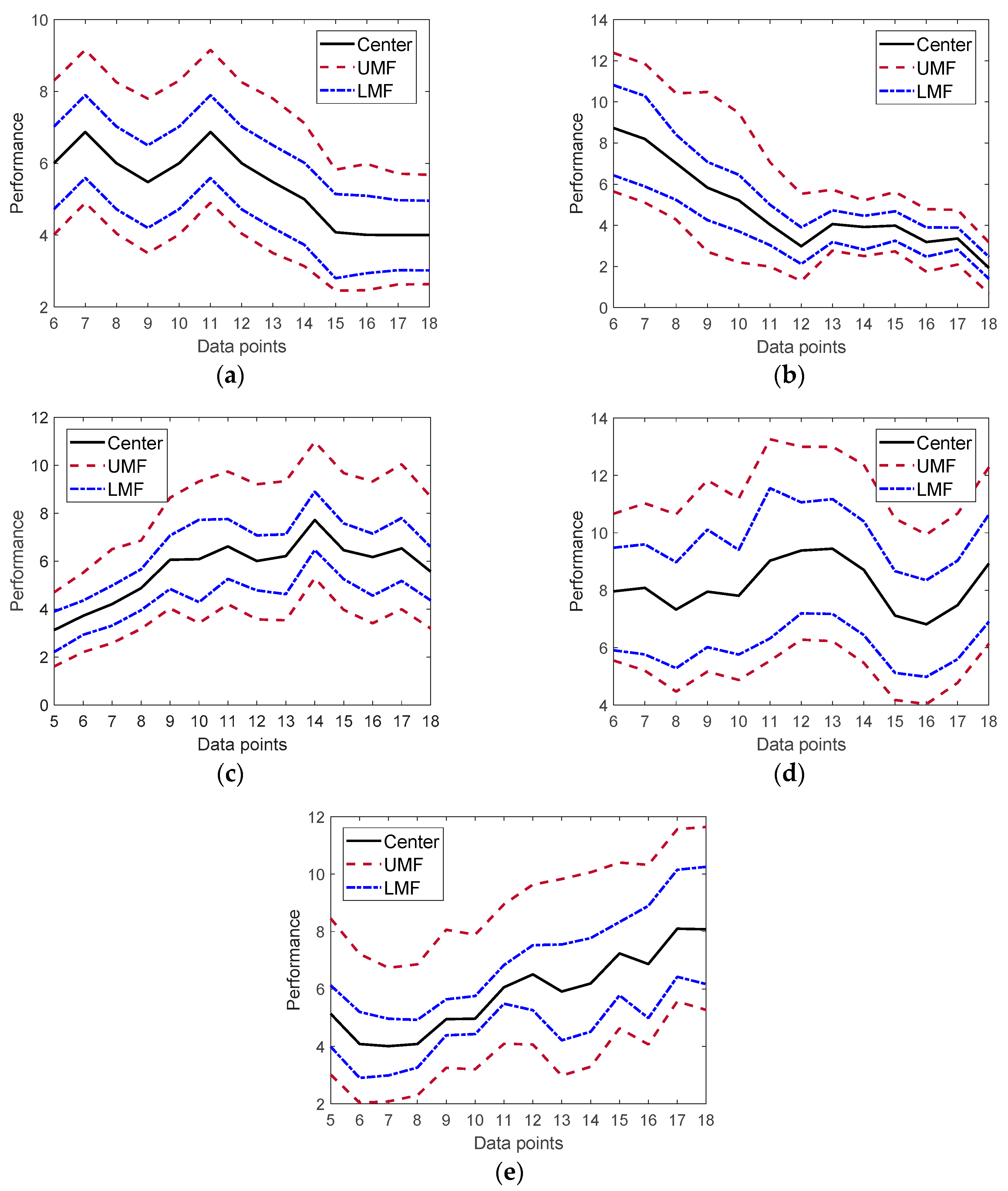
Despite its practicality, IT2F regression, which does not make use of FCM clustering and augmented input matrix as in the case of the proposed IT2F functions, cannot capture the trends and patterns in the historical dataset to the desired extent. Hence, both of the performance metrics were quite high. On the other hand, the proposed IT2F functions approach had successfully captured the patterns in the data thanks to its membership processing mechanisms. Figure 6 shows the estimated performance scores of the alternative 1 with respect to five criteria by means of the IT2F functions approach.
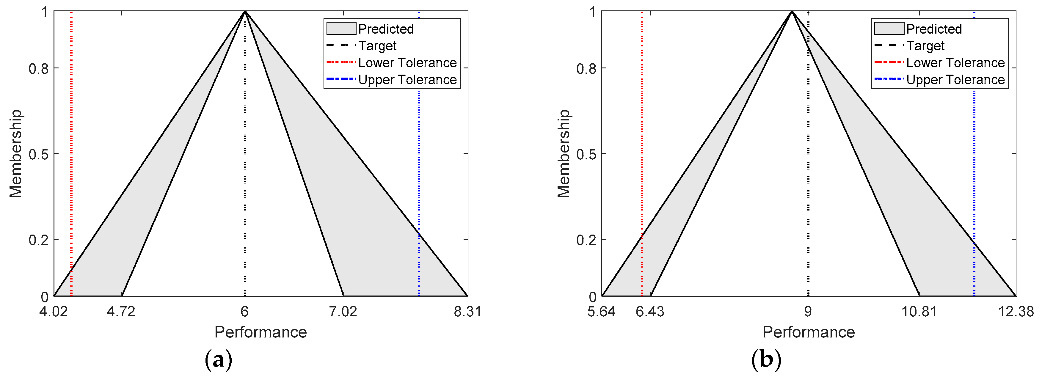
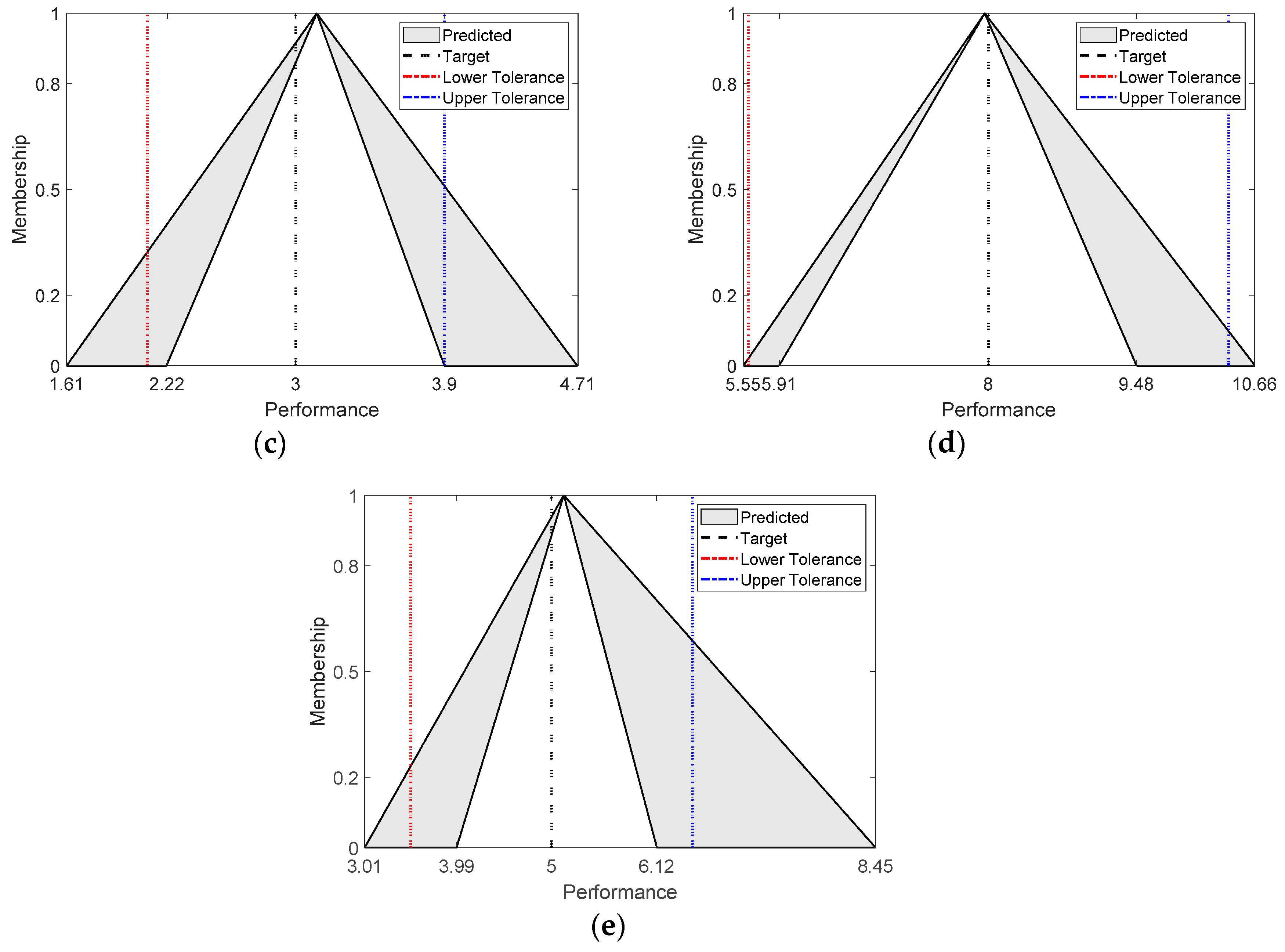
Note that the produced results were IT2F numbers. Another critical point is about whether the produced results satisfy the imposed constraints by possibility and necessity relationships. Figure 7 digs into the first data points of the predictions, which are illustrated in Figure 6. Note that the lower and upper tolerances covered the lower membership function, which was the property of the necessity constraints in the mathematical model. Furthermore, the lower and upper tolerances were covered by the upper membership function, which was due to the possibility constraints. It can be seen that both of the lower and upper tolerances lied within the FOU of the IT2F outputs. The estimated outputs were also inside the FOU and the centers of the IT2F outputs were quite close to the target values, which indicates the predictive power of the IT2F functions.
Based on the trained IT2F functions model, the current decision matrix was predicted. The resulting decision matrix is shown in Table 7.
As it is difficult for experts to interpret the produced results, they were transformed into linguistic terms in the next section.

4.3. Ranking of Employees

Step 10: In this step, a similarity-based vocabulary matching was performed. First, the linguistic terms and their corresponding IT2F number were determined. Table 8 shows the linguistic terms of the vocabulary.
Based on the linguistic terms given in Table 8, similarity-based vocabulary matching was carried out. As a result, the linguistic decision matrix is given in Table 9.
Step 11: When the linguistic decision matrix was formed, the results were presented to the decision makers. Then, the decision makers were asked to change the performance values of the alternatives based on their perceptions. The decision makers might accept the decision matrix as it is or alter the whole performance values depending on their judgments. In this study, decision makers decided to change the performance values of the second and third alternatives with respect to first, fourth, and fifth criteria. The modified decision matrix is represented in Table 10. The modified linguistic terms are highlighted by gray shading.
The decision makers accepted the linguistic terms produced by the IT2F functions model for the rest of the evaluations. By this way, required expert judgments were decreased by 80%, which dramatically increased the speed of decision making.
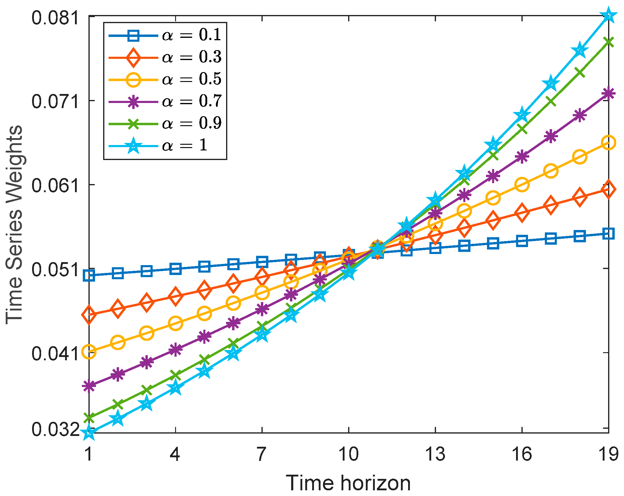
Step 12: In this step, time series weights were generated based on the BUM function. The only parameter required by BUM function was α . Figure 8 illustrates the time series weights for different α values. In this study, α was selected as 0.5. Furthermore, results for the different α values were examined as well.
Step 13: In this step, performance of each employee was evaluated at each period. Here, past and current decision matrices were evaluated one-by-one separately. As mentioned earlier, closeness coefficient is very practical to use so that for each period distance to positive and negative ideal solutions were calculated. The weights of criteria were assumed to be fixed throughout the periods and given as 0.10, 0.10, 0.15, 0.25, and 0.35, respectively. The separation measures are given in Table 11 and Table 12.
Based on the distances from positive and negative ideal solutions, closeness coefficients were calculated as given in Table 13.
Step 14: In this step, closeness coefficients pertaining to the past and current performance scores of employees were aggregated by taking into account the time series weights. As there were numerous aggregation operators, the most practical one, namely the DWA operator, was used in this study. As a result of the DWA operator, rankings of employees were obtained. Moreover, for the purpose of comparison, different model components were activated and the results were examined. Table 14 summarizes the computational setting with different model components.
The proposed model integrates all of the model components. Different from the proposed model, the predicted decision matrix was not modified in model 1. In model 2, neither the linguistic decision matrix was generated nor the decision makers were allowed to change the decision matrix. Finally, model 3 made use of the IT2F functions, vocabulary matching, and modified preferences, but only the decision matrix of the current period was considered for ranking of alternatives, which corresponded to the conventional MADM approach.
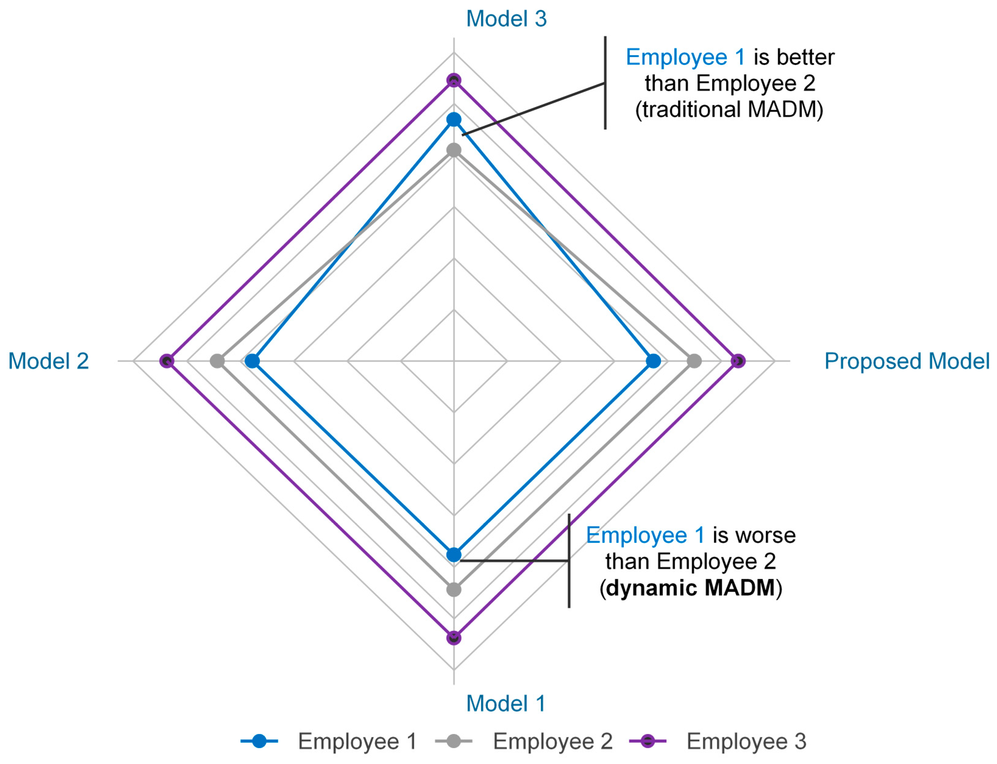
Step 15: The employees were ranked and the results were interpreted in this step. As can be seen from the Table 15, employee 3 dominated the other candidates regardless of the model configurations. However, the performance of employee 1 needed more attention here as the ranking order differed by the static or dynamic MADM aspects. The performance of employee 1 has been visualized in Figure 9.
It was observed that the performance of employee 2 was better than employee 1 for all of the dynamic MADM models. However, considering only the current decision matrix in model 3, static MADM ranked employee 1 as second and employee 2 as third.
Although the performance of the employee 1 was higher than the employee 2 in the current period, considering historical performance values changed the overall rankings. Therefore, the present study provided policy makers with a broader view regarding performance of employees by considering different modeling aspects.

5. Discussion

According to proposed dynamic MADM model, past performance values of employees were used to form current decision matrix. Hence, the current decision matrix was automatically generated based on the proposed IT2F functions model and the decision makers modified three performance scores out of 15. Therefore, preference elicitation procedures were dramatically improved.
The results of the case study had also shown that employee 3 had ranked first according to all of the dynamic MADM models. Although employee 1 had better performance than employee 2 in terms of current period performance, consideration of the past data made employee 1 the worst candidate for the full-time position among other employees. Although employee 2 had the worst performance without considering the past performance, with the dynamic character of the proposed model, employee 2 had become the second ranked alternative. As a result, taking into account the past and current decision matrices together provides more information to the decision makers and leads to more accurate rankings.

6. Conclusions

In this study, a new interactive dynamic MADM model, which combines IT2F regression and fuzzy functions approaches, was proposed. The proposed model exhibited desirable properties that helped overcome the drawbacks of the traditional dynamic MADM approaches. The proposed model was realized in a real-life personnel promotion problem. The proposed IT2F functions approach had improved the performance of IT2F regression by successfully capturing the trends and patterns in the historical records.
The advantage of the proposed model lies in its data-driven character, that is to say, the past data is used to guide preference elicitation processes. In classical MADM approaches, the decision makers are asked to fill out the entire decision matrix, which can be time consuming and cognitively demanding. On the other hand, the proposed model generates an IT2F decision matrix based on past data and allows decision makers to alter automatically generated decision matrix by using linguistic terms. Fuzziness in both the linguistic expressions and the past data were modeled by the proposed approach.
The main limitation of the presented study was that the results produced by the proposed model were highly dependent on the data obtained from the case company. Accordingly, results were difficult to be generalized. Secondly, prediction performance highly depends on available data. Nevertheless, the presented study can be improved in terms of many aspects. Hyper-parameter optimization can be used to tune the parameters of the model automatically. Different strategies can also be imposed to generate time series weights, and results can be compared. Last but not least, different MADM approaches can be used to rank the alternatives. In future studies, these considerations will be at the top of our agenda.

Author Contributions

The authors equally contributed to this work, thus they share first-author contribution. The authors contributed in the following manners: conceptualization, A.B. and İ.G.; methodology, A.B. and İ.G.; writing and original draft preparation, İ.G.; software, İ.G.; investigation, A.B.; supervision, A.B.; resources, A.B.; data curation, İ.G.; validation, A.B. and İ.G.

Funding

This research received no external funding.

Acknowledgments

We would like to thank the reviewers for their valuable comments.

Conflicts of Interest

The authors declare no conflict of interest.

References

  1. Dyer, J.S. Maut—Multiattribute Utility Theory. In Multiple Criteria Decision Analysis: State of the Art Surveys; Springer: New York, NY, USA, 2005; Volume 78, pp. 265–292. [Google Scholar]
  2. Fishburn, P.C. Utility Theory for Decision Making; Wiley: New York, NY, USA, 1970. [Google Scholar]
  3. Keeney, R.L. Building models of values. Eur. J. Oper. Res. 1988, 37, 149–157. [Google Scholar] [CrossRef]
  4. Saaty, T.L. The Analytic Hierarchy Process; McGraw-Hill: New York, NY, USA, 1980. [Google Scholar]
  5. Saaty, T.L. Decision Making with Dependence and Feedback: The Analytic Network Process; RWS Publications: Pittsburgh, PA, USA, 1996; p. 481. [Google Scholar]
  6. Hwang, C.L.; Yoon, K. Multiple Attribute Decision Making, Methods and Applications; Springer: New York, NY, USA, 1981; Volume 186. [Google Scholar]
  7. Roy, B. The Outranking Approach and the Foundations of Electre Methods. In Readings in Multiple Criteria Decision Aid; Bana e Costa, C., Ed.; Springer: Berlin/Heidelberg, Germany, 1990; pp. 155–183. [Google Scholar]
  8. Opricovic, S.; Tzeng, G.-H. Compromise solution by MCDM methods: A comparative analysis of VIKOR and TOPSIS. Eur. J. Oper. Res. 2004, 156, 445–455. [Google Scholar] [CrossRef]
  9. Fontela, E.; Gabus, A. The DEMATEL Observer; Battelle Geneva Research Center: Geneva, Switzerland, 1976. [Google Scholar]
  10. Kornbluth, J.S.H. Dynamic multi-criteria decision making. J. Multi-Criteria Decis. Anal. 1992, 1, 81–92. [Google Scholar] [CrossRef]
  11. Dong, Q.X.; Guo, Y.J.; He, Z.Y. Method of dynamic multi-criteria decision-making based on integration of absolute and relative differences. In Proceedings of the IEEE International Conference on Advanced Computer Control, Shenyang, China, 27–29 March 2010; pp. 353–356. [Google Scholar]
  12. Lou, C.; Peng, Y.; Kou, G.; Ge, X. DMCDM: A dynamic multi criteria decision making model for sovereign credit default risk evaluation. In Proceedings of the 2nd International Conference on Software Engineering and Data Mining, Chengdu, China, 23–25 June 2010; pp. 489–494. [Google Scholar]
  13. Campanella, G.; Ribeiro, R.A. A framework for dynamic multiple-criteria decision making. Decis. Support Syst. 2011, 52, 52–60. [Google Scholar] [CrossRef]
  14. Xu, Z.; Yager, R.R. Dynamic intuitionistic fuzzy multi-attribute decision making. Int. J. Approx. Reason. 2008, 48, 246–262. [Google Scholar] [CrossRef] [Green Version]
  15. Park, J.H.; Cho, H.J.; Kwun, Y.C. Extension of the VIKOR method to dynamic intuitionistic fuzzy multiple attribute decision making. Comput. Math. Appl. 2013, 65, 731–744. [Google Scholar] [CrossRef]
  16. Zhou, F.; Wang, X.; Samvedi, A. Quality improvement pilot program selection based on dynamic hybrid MCDM approach. Ind. Manag. Data Syst. 2018, 118, 144–163. [Google Scholar] [CrossRef]
  17. Bali, Ö.; Gümüş, S.; Kaya, İ. A Multi-Period Decision Making Procedure Based on Intuitionistic Fuzzy Sets for Selection Among Third-Party Logistics Providers. J. Mult. Valued Log. Soft Comput. 2015, 24, 547–569. [Google Scholar]
  18. Chen, Y.; Li, B. Dynamic multi-attribute decision making model based on triangular intuitionistic fuzzy numbers. Sci. Iran. 2011, 18, 268–274. [Google Scholar] [CrossRef] [Green Version]
  19. Liang, C.Y.; Zhang, E.Q.; Qi, X.W.; Cai, M.J. A dynamic multiple attribute decision making method under incomplete information. In Proceedings of the 6th International Conference on Natural Computation, Yantai, China, 10–12 August 2010; pp. 2720–2723. [Google Scholar]
  20. Bali, O.; Dagdeviren, M.; Gumus, S. An integrated dynamic intuitionistic fuzzy MADM approach for personnel promotion problem. Kybernetes 2015, 44, 1422–1436. [Google Scholar] [CrossRef]
  21. Xu, Z. A method based on the dynamic weighted geometric aggregation operator for dynamic hybrid multi-attribute group decision making. Int. J. Uncertain. Fuzziness Knowl. Based Syst. 2009, 17, 15–33. [Google Scholar] [CrossRef]
  22. Zulueta, Y.; Martínez-Moreno, J.; Pérez, R.B.; Martínez, L. A discrete time variable index for supporting dynamic multi-criteria decision making. Int. J. Uncertain. Fuzziness Knowl. Based Syst. 2014, 22, 1–22. [Google Scholar] [CrossRef]
  23. Lin, Y.-H.; Lee, P.-C.; Ting, H.-I. Dynamic multi-attribute decision making model with grey number evaluations. Expert Syst. Appl. 2008, 35, 1638–1644. [Google Scholar] [CrossRef]
  24. Zhang, C.L. Risk assessment of supply chain finance with intuitionistic fuzzy information. J. Intell. Fuzzy Syst. 2016, 31, 1967–1975. [Google Scholar] [CrossRef]
  25. Wei, G.W. Some geometric aggregation functions and their application to dynamic multiple attribute decision making in the intuitionistic fuzzy setting. Int. J. Uncertain. Fuzziness Knowl. Based Syst. 2009, 17, 179–196. [Google Scholar] [CrossRef]
  26. Ai, F.Y.; Yang, J.Y. Approaches to dynamic multiple attribute decision making with 2-tuple linguistic information. J. Intell. Fuzzy Syst. 2014, 27, 2715–2723. [Google Scholar] [CrossRef]
  27. Liu, H.; Jiang, L.; Martínez, L. A dynamic multi-criteria decision making model with bipolar linguistic term sets. Expert Syst. Appl. 2018, 95, 104–112. [Google Scholar] [CrossRef]
  28. Liu, Y. A method for 2-tuple linguistic dynamic multiple attribute decision making with entropy weight. J. Intell. Fuzzy Syst. 2014, 27, 1803–1810. [Google Scholar] [CrossRef]
  29. Zulueta-Veliz, Y.; Sanchez, P.J. Linguistic dynamic multicriteria decision making using symbolic linguistic computing models. Granul. Comput. 2018. [Google Scholar] [CrossRef]
  30. Xu, Z. Multi-period multi-attribute group decision-making under linguistic assessments. Int. J. Gen. Syst. 2009, 38, 823–850. [Google Scholar] [CrossRef]
  31. Cui, J.; Liu, S.F.; Dang, Y.G.; Xie, N.M.; Zeng, B. A grey multi-stage dynamic multiple attribute decision making method. In Proceedings of the IEEE International Conference on Grey Systems and Intelligent Services, Nanjing, China, 15–18 September 2011; pp. 548–550. [Google Scholar]
  32. Shen, J.M.; Dang, Y.G.; Zhou, W.J.; Li, X.M. Evaluation for Core Competence of Private Enterprises in Xuchang City Based on an Improved Dynamic Multiple-Attribute Decision-Making Model. Math. Probl. Eng. 2015, 2015. [Google Scholar] [CrossRef]
  33. Mardani, A.; Nilashi, M.; Zavadskas, E.K.; Awang, S.R.; Zare, H.; Jamal, N.M. Decision Making Methods Based on Fuzzy Aggregation Operators: Three Decades Review from 1986 to 2017. Int. J. Inf. Technol. Decis. Mak. 2018, 17, 391–466. [Google Scholar] [CrossRef]
  34. Saaty, T.L. Time dependent decision-making; dynamic priorities in the AHP/ANP: Generalizing from points to functions and from real to complex variables. Math. Comput. Model. 2007, 46, 860–891. [Google Scholar] [CrossRef]
  35. Hashemkhani Zolfani, S.; Maknoon, R.; Zavadskas, E.K. An introduction to Prospective Multiple Attribute Decision Making (PMADM). Technol. Econ. Dev. Econ. 2016, 22, 309–326. [Google Scholar] [CrossRef]
  36. Orji, I.J.; Wei, S. An innovative integration of fuzzy-logic and systems dynamics in sustainable supplier selection: A case on manufacturing industry. Comput. Ind. Eng. 2015, 88, 1–12. [Google Scholar] [CrossRef]
  37. Baykasoğlu, A.; Gölcük, İ. A dynamic multiple attribute decision making model with learning of fuzzy cognitive maps. Comput. Ind. Eng. 2019. [Google Scholar] [CrossRef]
  38. Lee, H.; Tanaka, H. Fuzzy approximations with non-symmetric fuzzy parameters in fuzzy regression analysis. J. Oper. Res. Soc. Jpn. 1999, 42, 98–112. [Google Scholar] [CrossRef]
  39. Turksen, I.B. Fuzzy functions with LSE. Appl. Soft Comput. J. 2008, 8, 1178–1188. [Google Scholar] [CrossRef]
  40. Çelikyilmaz, A.; Turksen, I.B. Fuzzy functions with support vector machines. Inf. Sci. 2007, 177, 5163–5177. [Google Scholar] [CrossRef]
  41. Kasabov, N.K.; Song, Q. DENFIS: Dynamic evolving neural-fuzzy inference system and its application for time-series prediction. IEEE Trans. Fuzzy Syst. 2002, 10, 144–154. [Google Scholar] [CrossRef]
  42. Emami, M.R.; Türksen, I.B.; Goldenberg, A.A. Development of a systematic methodology of fuzzy logic modeling. IEEE Trans. Fuzzy Syst. 1998, 6, 346–361. [Google Scholar] [CrossRef]
  43. Kilic, K.; Sproule, B.A.; Turksen, I.B.; Naranjo, C.A. A fuzzy system modeling algorithm for data analysis and approximate reasoning. Robot. Auton. Syst. 2004, 49, 173–180. [Google Scholar] [CrossRef]
  44. Babuška, R.; Verbruggen, H.B. Constructing fuzzy models by product space clustering. In Fuzzy Model Identification; Springer: Berlin, Germany, 1997; pp. 53–90. [Google Scholar]
  45. Zarandi, M.H.F.; Turksen, I.B.; Rezaee, B. A systematic approach to fuzzy modeling for rule generation from numerical data. In Proceedings of the IEEE Annual Meeting of the Fuzzy Information, Banff, AB, Canada, 27–30 June 2004; pp. 768–773. [Google Scholar]
  46. Jang, J.-S.R. ANFIS: Adaptive-network-based fuzzy inference system. IEEE Trans. Syst. Man Cybern. 1993, 23, 665–685. [Google Scholar] [CrossRef]
  47. Cordón, O.; Gomide, F.; Herrera, F.; Hoffmann, F.; Magdalena, L. Ten years of genetic fuzzy systems: Current framework and new trends. Fuzzy Sets Syst. 2004, 141, 5–31. [Google Scholar] [CrossRef]
  48. Mendel, J.M.; John, R.I.; Feilong, L. Interval Type-2 Fuzzy Logic Systems Made Simple. IEEE Trans. Fuzzy Syst. 2006, 14, 808–821. [Google Scholar] [CrossRef]
  49. Mendel, J.M.; Wu, D. Perceptual Computing: Aiding People in Making Subjective Judgments; Wiley-IEEE Press: Hoboken, NJ, USA, 2010; Volume 13. [Google Scholar]
  50. Hamrawi, H.; Coupland, S. Type-2 fuzzy arithmetic using alpha-planes. In Proceedings of the IFSA-EUSFLAT Conference, Lisbon, Portugal, 20–24 July 2009; pp. 606–612. [Google Scholar]
  51. Chen, S.-M.; Yang, M.-W.; Lee, L.-W.; Yang, S.-W. Fuzzy multiple attributes group decision-making based on ranking interval type-2 fuzzy sets. Expert Syst. Appl. 2012, 39, 5295–5308. [Google Scholar] [CrossRef]
  52. Karnik, N.N.; Mendel, J.M. Centroid of a type-2 fuzzy set. Inf. Sci. 2001, 132, 195–220. [Google Scholar] [CrossRef]
  53. Wu, D.; Mendel, J.M. A comparative study of ranking methods, similarity measures and uncertainty measures for interval type-2 fuzzy sets. Inf. Sci. 2009, 179, 1169–1192. [Google Scholar] [CrossRef]
  54. Bajestani, N.S.; Kamyad, A.V.; Esfahani, E.N.; Zare, A. Prediction of retinopathy in diabetic patients using type-2 fuzzy regression model. Eur. J. Oper. Res. 2018, 264, 859–869. [Google Scholar] [CrossRef]
  55. Yager, R.R. On ordered weighted averaging aggregation operators in multicriteria decisionmaking. IEEE Trans. Syst. Man Cybern. 1988, 18, 183–190. [Google Scholar] [CrossRef]
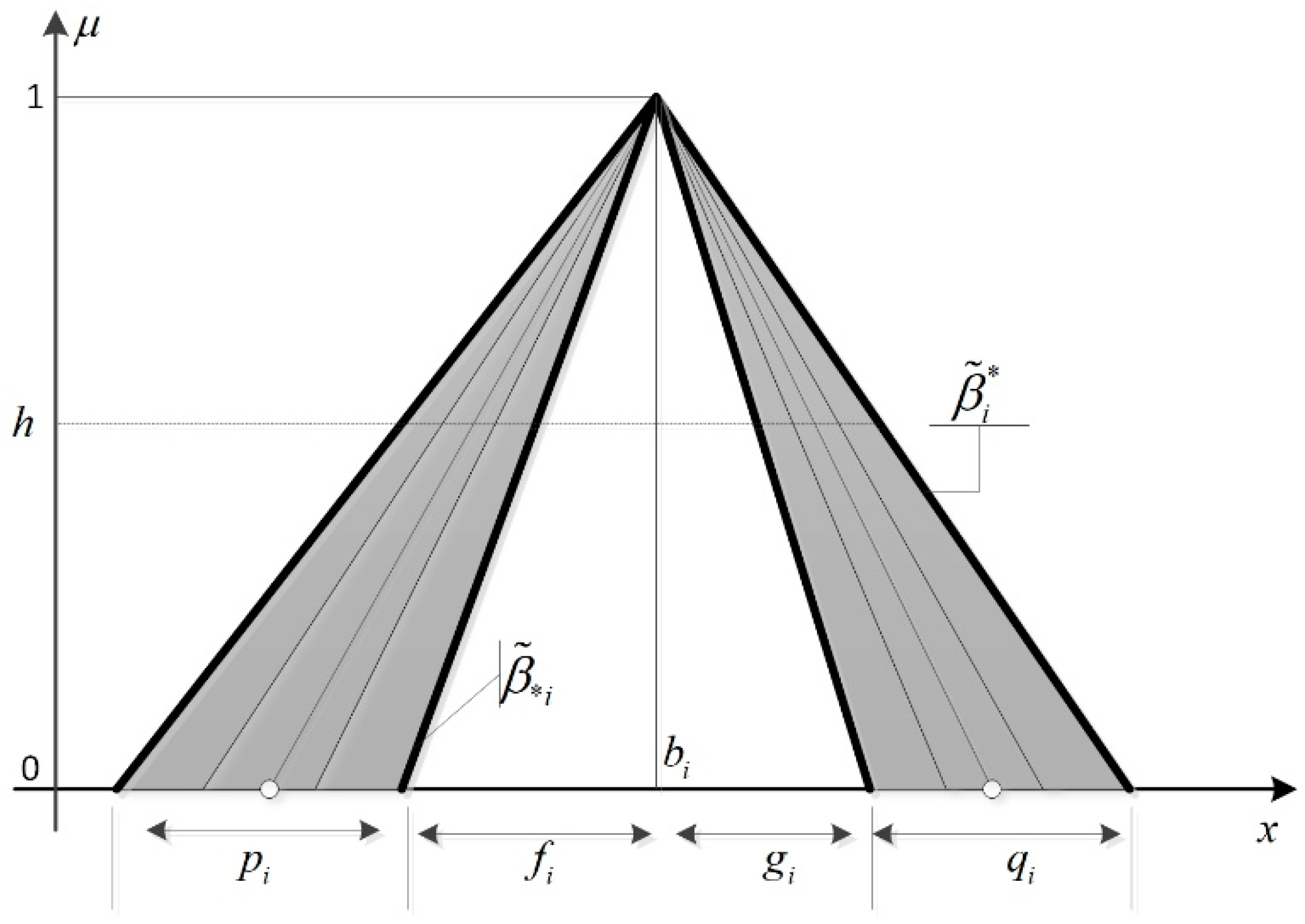
Figure 1. Representation of regression coefficients.
Mathematics 07 00584 g001
Figure 2. Flowchart of the proposed model.
Mathematics 07 00584 g002
Figure 3. Proposed IT2F functions approach.
Mathematics 07 00584 g003
Figure 4. Interactive process of the proposed model.
Mathematics 07 00584 g004
Figure 5. Decision hierarchy.
Mathematics 07 00584 g005
Figure 6. Estimations for the 1st alternative. (a) 1st criterion; (b) 2nd criterion; (c) 3rd criterion; (d) 4th criterion and (e) 5th criterion.
Mathematics 07 00584 g006
Figure 7. Details of the predictions for the 1st alternative. (a) 6th data point w.r.t. 1st criterion; (b) 6th data point w.r.t. 2nd criterion; (c) 5th data point w.r.t. 3rd criterion; (d) 6th data point w.r.t. 4th criterion and (e) 5th data point w.r.t. 5th criterion.
Mathematics 07 00584 g007aMathematics 07 00584 g007b
Figure 8. Time series weights.
Mathematics 07 00584 g008
Figure 9. Changes in the ranking of employee 1.
Mathematics 07 00584 g009
Table 1. Illustration of the four-period example.
PeriodPast Decision MatricesCorresponding Time SeriesInput MatrixOutput Matrix
t1 A 1 A 2 A 3 C 1 [ a 12 ( t 1 ) = 5 ] [ y 1 = 5 y 2 = 3 y 3 = 6 y 4 = 8 ] X = [ y 1 y 2 y 2 y 3 ] = [ 5 3 3 6 ] Y = [ y 3 y 4 ] = [ 6 8 ]
t2 A 1 A 2 A 3 C 1 [ a 12 ( t 2 ) = 3 ]
t3 A 1 A 2 A 3 C 1 [ a 12 ( t 3 ) = 6 ]
t4 A 1 A 2 A 3 C 1 [ a 12 ( t 4 ) = 8 ]
Note that because the lagged periods are two, number of data points is H p = 4 2 = 2 .
Table 2. Historical data of employee 1.
PeriodC1C2C3C4C5
167337
267226
378335
469455
568365
669484
778484
867574
966685
1065685
1174796
12636106
13546106
1454886
1544678
1643677
1743678
1842698
Table 3. Parameters of the model.
AlternativeCriteriaParameters
cmLagged_Periods
1121.65
251.65
342.14
452.15
541.64
2141.65
252.15
321.15
452.15
551.65
3122.15
221.65
331.65
452.15
551.65
Table 4. Cluster 1 results for the 1st alternative and 1st criteria.
VariableIT2F Regression CoefficientsIT2F Coefficients
bfgpq
110.5728.65 × 10−90.0319.30 × 10−119.13 × 10⁻¹¹((10.572, 10.572, 10.603;1),
(10.572, 10.572, 10.603;1))
μ −8.5243.39 × 10−90.0706.45 × 10−116.44 × 10⁻¹¹((−8.524, −8.524, −8.454;1),
(−8.524, −8.524, −8.454;1))
exp ( μ ) −4.5502.04 × 10−90.0162.79 × 10−112.78 × 10⁻¹¹((−4.55, −4.55, −4.534;1),
(−4.55, −4.55, −4.534;1))
μ 2 13.4667.27 × 10−90.0857.34 × 10−117.34 × 10⁻¹¹((13.466, 13.466, 13.551;1),
(13.466, 13.466, 13.551;1))
x t 1 0.0170.1460430.0102.67 × 10−112.59 × 10⁻¹¹((−0.129, 0.017, 0.027;1),
(−0.129, 0.017, 0.027;1))
x t 2 −0.6131.24 × 10−90.0050.10.185714((−0.713, −0.613, −0.423;1),
(−0.613, −0.613, −0.609;1))
x t 3 −0.2111.44 × 10−90.0041.67 × 10−111.63 × 10⁻¹¹((−0.211, −0.211, −0.207;1),
(−0.211, −0.211, −0.207;1))
x t 4 0.8220.0781110.1261.48 × 10−111.42 × 10⁻¹¹((0.744, 0.822, 0.948;1),
(0.744, 0.822, 0.948;1))
x t 5 0.0381.44 × 10−90.0061.36 × 10−111.34 × 10⁻¹¹((0.038, 0.038, 0.044;1),
(0.038, 0.038, 0.044;1))
Table 5. Cluster-2 results for the 1st alternative and 1st criteria.
VariableIT2F Regression CoefficientsIT2F Coefficients
bfgpq
1−10.9071.281.0184.25 × 10−94.59 × 10⁻⁹((−12.184, −10.907, −9.889;1),
(−12.184, −10.907, −9.889;1))
μ −18.9643.03 × 10−90.0001.44 × 10−81.44 × 10⁻⁸((−18.964, −18.964, −18.964;1),
(−18.964, −18.964, −18.964;1))
exp ( μ ) 15.0771.79 × 10−90.0003.39 × 10−93.61 × 10⁻⁹((15.077, 15.077, 15.077;1),
(15.077, 15.077, 15.077;1))
μ 2 −3.4473.12 × 10−90.0007.20 × 10−11.16((−4.167, −3.447, −2.289;1),
(−3.447, −3.447, −3.447;1))
x t 1 −0.1071.50 × 10−90.0008.08 × 10−108.56 × 10⁻¹⁰((−0.107, −0.107, −0.107;1),
(−0.107, −0.107, −0.107;1))
x t 2 −0.7259.06 × 10−100.0003.64 × 10−70.024974((−0.725, −0.725, −0.7;1),
(−0.725, −0.725, −0.725;1))
x t 3 −0.2623.18 × 10−90.0006.04 × 10−106.37 × 10⁻¹⁰((−0.262, −0.262, −0.262;1),
(−0.262, −0.262, −0.262;1))
x t 4 0.7353.18 × 10−90.0005.26 × 10−105.27 × 10⁻¹⁰((0.735, 0.735, 0.735;1),
(0.735, 0.735, 0.735;1))
x t 5 0.1501.16 × 10−50.0015.74 × 10−106.10 × 10⁻¹⁰((0.15, 0.15, 0.151;1),
(0.15, 0.15, 0.151;1))
Table 6. Performance comparison of the proposed method and IT2F regression.
AlternativeCriteriaProposed IT2F FunctionsIT2F Regression
RMSEMAPERMSEMAPE
110.23072.38830.697411.4445
20.19483.31490.784415.1122
30.25194.06790.982814.0217
40.3753.44590.69527.2826
50.36065.64630.897616.7376
210.28946.06870.444913.6456
20.23922.43060.67937.5079
30.37334.28110.934311.083
40.42835.16770.59347.8132
50.30354.00270.56577.9788
310.14571.7220.72858.0463
20.16863.99120.583317.4631
30.24172.63020.61966.6876
40.21422.1350.32213.4379
50.22052.74940.55677.9517
Table 7. Resulting decision matrix of the IT2F functions.
CriteriaAlternatives
A1A2A3
C1((1.694, 2.99, 4.515;1),((2.163, 3.73, 5.516;1),((5.223, 7.902, 11.27;1),
(2.064, 2.99, 3.822;1))(2.864, 3.73, 4.204;1))(5.601, 7.902, 10.396;1))
C2((1.354, 2.255, 3.33;1),((4.992, 8.419, 12.522;1),((2.662, 3.919, 5.449;1),
(1.891, 2.255, 2.623;1))(5.964, 8.419, 10.802;1))(3.204, 3.919, 4.596;1))
C3((2.986, 5.358, 8.46;1),((2.194, 4.143, 5.991;1),((6.016, 9.229, 12.788;1),
(4.13, 5.358, 6.362;1))(3.144, 4.143, 5.238;1))(6.68, 9.229, 11.589;1))
C4((7.187, 10.353, 14.08;1),((0.469, 1.617, 3.242;1),((5.678, 8.415, 11.417;1),
(8.084, 10.353, 12.123;1))(0.933, 1.617, 2.178;1))(6.071, 8.415, 10.508;1))
C5((2.409, 5.252, 9.04;1),((4.427, 6.446, 9.052;1),((3.715, 6.246, 8.94;1),
(3.372, 5.252, 7.208;1))(5.168, 6.446, 7.487;1))(4.566, 6.246, 7.472;1))
Table 8. Vocabulary of linguistic terms.
Linguistic TermsIT2F Number
SymbolExplanation
VLVery Low((0, 0, 1;1), (0, 0, 0.5;1))
LLow((0, 1, 3;1), (0.5, 1, 2;1))
MLMedium Low((1, 3, 5;1), (2, 3, 4;1))
MMedium((3, 5, 7;1), (4, 5, 6;1))
MHMedium High((5, 7, 9;1), (6, 7, 8;1))
HHigh((7, 9, 10;1), (8, 9, 9.5;1))
VHVery High((9, 10, 10;1), (9.5, 10, 10;1))
Table 9. Linguistic decision matrix.
CriteriaAlternatives
A1A2A3
C1MLMLMH
C2MLHML
C3MMH
C4HLH
C5MMHMH
Table 10. Modified decision matrix.
CriteriaAlternatives
A1A2A3
C1MLMHMH
C2MLHML
C3MMH
C4HLMH
C5MHMH
Table 11. Distances between the performance of employees and the positive ideal solution.
PeriodsDistance to Positive Ideal Solution
Employee 1Employee 2Employee 3
t10.14580.11010.1111
t20.22590.15690.1084
t30.21550.15460.1161
t40.16040.12030.0850
t50.17300.13130.0938
t60.17000.09190.0833
t70.17000.09770.0750
t80.17140.07090.0643
t90.12560.08720.0750
t100.13030.08740.0750
t110.09600.07970.1086
t120.11460.09010.1397
t130.12040.09610.1393
t140.10040.09140.1050
t150.12260.14010.0797
t160.12640.13300.0972
t170.14220.18730.1001
t180.14040.23350.0981
tC0.17250.19550.1143
Table 12. Distances between the performance of employees and the negative ideal solution.
PeriodsDistance to Negative Ideal Solution
Employee 1Employee 2Employee 3
t10.14090.15560.1541
t20.11690.15240.2462
t30.11610.13340.2155
t40.08980.06980.1613
t50.09950.08050.1762
t60.10110.16360.1836
t70.09830.12780.1857
t80.07440.16970.1807
t90.06840.12590.1385
t100.05630.09500.1336
t110.08110.11020.0717
t120.09970.13970.0750
t130.08170.13110.0750
t140.06800.10500.0914
t150.09270.08500.1247
t160.08100.10000.1244
t170.12180.10500.1719
t180.21430.11730.1966
tC0.18730.16310.1751
Table 13. Closeness coefficients of employees.
PeriodsCloseness Coefficients
Employee 1Employee 2Employee 3
t10.49150.58560.5811
t20.34110.49280.6942
t30.35010.46330.6499
t40.35880.36710.6549
t50.36520.38010.6527
t60.37290.64050.6878
t70.36640.56660.7123
t80.30280.70530.7376
t90.35250.59070.6487
t100.30160.52080.6404
t110.45800.58020.3978
t120.46520.60780.3493
t130.40430.57690.3500
t140.40390.53470.4653
t150.43040.37760.6099
t160.39060.42910.5614
t170.46130.35930.6321
t180.60410.33450.6671
tC0.52060.45470.6051
Table 14. Different model configurations.
Model ComponentsModels
Proposed ModelModel 1Model 2Model 3
IT2F FunctionsYesYesYesYes
Vocabulary MatchingYesYesNoYes
Modified preferences (interactive)YesNoNoYes
DWA OperatorYesYesYesNo
Table 15. Overall results.
ModelOverall Assessment
Employee 1Employee 2Employee 3
CCRankCCRankCCRank
Proposed Model0.413830.498420.58951
Model 10.417630.492620.59671
Model 20.418530.490520.59511
Model 30.520620.454730.60511