Audio Signal Processing Using Fractional Linear Prediction

Abstract

Fractional linear prediction (FLP), as a generalization of conventional linear prediction (LP), was recently successfully applied in different fields of research and engineering, such as biomedical signal processing, speech modeling and image processing. The FLP model has a similar design as the conventional LP model, i.e., it uses a linear combination of “fractional terms” with different orders of fractional derivative. Assuming only one “fractional term” and using limited number of previous samples for prediction, FLP model with “restricted memory” is presented in this paper and the closed-form expressions for calculation of FLP coefficients are derived. This FLP model is fully comparable with the widely used low-order LP, as it uses the same number of previous samples, but less predictor coefficients, making it more efficient. Two different datasets, MIDI Aligned Piano Sounds (MAPS) and Orchset, were used for the experiments. Triads representing the chords composed of three randomly chosen notes and usual Western musical chords (both of them from MAPS dataset) served as the test signals, while the piano recordings from MAPS dataset and orchestra recordings from the Orchset dataset served as the musical signal. The results show enhancement of FLP over LP in terms of model complexity, whereas the performance is comparable.

1. Introduction

The sinusoidal model is widely used for representation of pseudo-stationary signals, especially in audio coding [1] and musical signal processing [2]. Parameters of the sinusoidal model are determined frame-wise from the input audio/musical signal, and a sound is synthesized using the extracted parameters [3]. A pure tone can be represented as a single sine wave, whereas the musical chords are produced by combining three or more sine waves with different frequencies. In fact, any musical tone can be described as a combination of sine waves or its partials, each with its own amplitude, phase and frequency of vibration [4]. A sine wave can be fully described using three parameters: amplitude, phase and frequency. Obviously, such signal is redundant; hence, there is no need to encode and transmit each signal sample.

Linear prediction (LP) can be used to remove redundancy by predicting the current signal sample from the signal history, as the weighted linear combination of past samples. In that case, only the coefficients of the predictor need to be transmitted, not the signal samples themselves. While LP is extensively used for modeling speech signal [5,6,7], it did not prove to be the best choice for modeling audio signals. This is unexpected, since a signal represented by a combination of sine waves should be perfectly predicted using an LP model with an order twice larger than the number of sinusoids. The problem might be the fact that LP can model well signals with equally distributed tonal components in the Nyquist interval, which is not the case with audio, where tonal components are concentrated in a substantially smaller frequency region in comparison to the signal bandwidth [8]. This happens due to the fact that audio signals are usually sampled at a much higher frequency than the frequency of their tonal components. Nevertheless, there are applications of LP in audio coding algorithms using the so-called frequency-warped LP [9,10], where the unit delays are replaced by the first-order all-pass filter elements to adjust the frequency resolution in the spectral estimate to closely approximate the frequency resolution of human hearing [9]. LP is also used in acoustic echo cancelation [11], music dereverberation [12], audio signal classification [13] and audio/music onset detection [14,15].

The idea of using the signal history is fundamentally rooted in fractional calculus [16]. Fractional linear prediction (FLP), as a generalization of LP for fractional (arbitrary real) order derivatives, was recently used in electroencephalogram (EEG) [16,17] and electrocardiogram (ECG) signal modeling [18], as well as in speech coding [16,19,20,21]. While in [17,18,19] the full signal history is used for predicting the current signal sample, which is impractical from the implementation point of view, a model with restricted signal memory that uses only the recent signal samples and its applications is proposed in [21,22]. However, to the best of our knowledge, there are no applications of FLP in audio/musical signal processing. In this paper, we present FLP with memory restricted to maximum of four previous samples and apply it to prediction of randomly generated test chords, usual chords in Western music and piano parts extracted from the MIDI Aligned Piano Sounds dataset; and musical parts extracted from symphonies, ballets and other classical musical forms, and interpreted by symphonic orchestras, from the Orchset dataset.

The paper is organized as follows. Section 2 presents an overview of conventional LP and the FLP with “restricted memory”. Datasets used for experiments are described in Section 3. The numerical results using the test chords, piano and orchestra musical parts are discussed in Section 4, followed by concluding remarks in Section 5.

2. Linear Prediction

2.1. Conventional Linear Prediction

Let the signal $x\left(t\right)$ represent a linear and stationary stochastic process, where $x_{\left[n\right]}=x\left(nT\right)$ is the nth signal sample at arbitrary time t, and T is the sampling period. The signal $x\left(t\right)$ at time instance $t=nT$ is modeled as the linear combination of p previous signal samples:

$${\widehat{x}}_{\left[n\right]}=\sum _{i=1}^p{a}_i{x}_{[n-i]},$$

(1)

where ${\widehat{x}}_{\left[n\right]}$ denotes the predicted signal sample and $a_i$ are the linear predictor coefficients. The order of a linear predictor denotes the number of linear predictor coefficients, which is equal to the number of samples used for prediction.

The prediction error $e_{\left[n\right]}=x_{\left[n\right]}-{\widehat{x}}_{\left[n\right]}$ is defined as the deviation of the predicted signal $\widehat{x}$ from the original signal x, and the mean-squared prediction error is equal to:

$$J=E\left[e_{\left[n\right]}^2\right]=E{\left[x_{\left[n\right]}-\sum _{i=1}^p{a}_i{x}_{[n-i]}\right]}^2,$$

(2)

where $E[·]$ is the mathematical expectation. The optimal predictor coefficients $a_i$ can be determined by equating the first derivative of J, with respect to $a_i$, to zero. After some manipulation, we obtain:

$$\sum _{i=1}^p{a}_i{R}_{xx}(k-i)=R_{xx}\left(k\right),k=1,2,\dots ,p,$$

(3)

where $R_{xx}\left(k\right)=E\left[x_{\left[n\right]}{x}_{[n-k]}\right]$ denotes the autocorrelation function at lag k. Equation (3) is known as the Yule–Walker equation [7] and can be rewritten in the matrix form as:

$${\mathbf{R}}_{xx}·\mathbf{a}={\mathbf{r}}_{xx},$$

(4)

where

$${\mathbf{R}}_{xx}=\left[\begin{array}{ccccc}{R}_{xx}\left(0\right)& R_{xx}\left(1\right)& R_{xx}\left(2\right)& \cdots & R_{xx}(p-1)\\ R_{xx}\left(1\right)& R_{xx}\left(2\right)& R_{xx}\left(3\right)& \cdots & R_{xx}(p-2)\\ ⋮& ⋮& ⋮& \ddots & ⋮\\ R_{xx}(p-1)& R_{xx}(p-2)& R_{xx}(p-3)& \cdots & 0\end{array}\right],$$

$$\mathbf{a}={\left[a_1{a}_2{a}_3\cdots a_p\right]}^T,$$

$${\mathbf{r}}_{xx}={\left[R_{xx}\left(1\right)R_{xx}\left(2\right)R_{xx}\left(3\right)\cdots R_{xx}\left(p\right)\right]}^T.$$

The optimal linear predictor coefficients $\mathbf{a}$ can be found from:

$$\mathbf{a}={{\mathbf{R}}_{xx}}^{-1}·{\mathbf{r}}_{xx}.$$

(5)

2.2. Fractional Linear Prediction with “Restricted Memory”

FLP is a generalization of LP using the fractional-order derivatives. Using the analogy from LP, the nth signal sample can be represented as the linear combination of q “fractional terms”, and can be written as [16]:

$${\widehat{x}}_{\left[n\right]}=\sum _{i=1}^q{a}_i{D}^{{\alpha }_i}{x}_{[n-1]},$$

(6)

where ${\widehat{x}}_{\left[n\right]}$ is the estimate of the nth signal sample, q is the number of “fractional terms” used for the prediction, $a_i$ are the FLP coefficients, and $D^{\alpha }{x}_{[n-1]}$ are the fractional derivatives of order ${\alpha }_i$ of the time-delayed signal, where ${\alpha }_i\in \mathbb{R}$.

The fractional derivative $D^{\alpha }$ can be approximated by the Grünwald–Letnikov (GL) definition of a function $x\left(t\right)$ at time instant t [23]:

$${}_a{D}_t^{\alpha }x\left(t\right)=\underset{h\to 0}{lim}\frac{1}{h^{\alpha }}\sum _{j=0}^{⌊\frac{t-a}{h}⌋}{(-1)}^j\left(\genfrac{}{}{0pt}{}{\alpha }{j}\right)x(t-jh),$$

(7)

where h is the sampling period, a and t are lower and upper limits of differentiation, and $\alpha \in \mathbb{R}$ is the order of fractional differentiation. Note that the upper limit of summation tends to infinity. Accounting only for the recent history of the signal, i.e., replacing the lower limit a by the the moving lower limit $t-L$ (L is the memory length), the “short memory” principle [23] is employed. Due to this approximation, the number of addends in Equation (7) is not greater than $K=⌊L/h⌋$. For $t=nh$, Equation (7) becomes:

$$D^{\alpha }x\left(nh\right)=\underset{h\to 0}{lim}\frac{1}{h^{\alpha }}\sum _{j=0}^K{(-1)}^j\left(\genfrac{}{}{0pt}{}{\alpha }{j}\right)x\left((n-j)h\right).$$

(8)

Replacing $x\left(nh\right)$ with $x_{\left[n\right]}$, and assuming that in the signal prediction only the past samples are used for the estimation of the predicted signal sample, without including the current sample, i.e., introducing a time-delay in Equation (8) of one sample, one gets:

$$D^{\alpha }{x}_{[n-1]}=h^{-\alpha }\sum _{j=0}^K{(-1)}^j\left(\genfrac{}{}{0pt}{}{\alpha }{j}\right)x_{[n-1-j]}.$$

(9)

Taking into account only one “fractional term” from Equation (6), i.e., when $q=1$, one obtains [21,22]:

$${\widehat{x}}_{\left[n\right]}=a{D}^{\alpha }{x}_{[n-1]}.$$

(10)

Considering $K\in \mathbb{I}$ as the upper limit of the summation in Equation (9), i.e., for $K=1$:

$$D^{\alpha }{x}_{[n-1]}=\frac{1}{h^{\alpha }}\left(x_{[n-1]}-\alpha x_{[n-2]}\right),$$

(11)

$K=2$:

$$D^{\alpha }{x}_{[n-1]}=\frac{1}{h^{\alpha }}\left(x_{[n-1]}-\alpha x_{[n-2]}-\frac{\alpha (1-\alpha )}{2}{x}_{[n-3]}\right),$$

(12)

and $K=3$:

$$D^{\alpha }{x}_{[n-1]}=\frac{1}{h^{\alpha }}\left(x_{[n-1]}-\alpha x_{[n-2]}-\frac{\alpha (1-\alpha )}{2}\left(x_{[n-3]}+\frac{2-\alpha }{3}{x}_{[n-4]}\right)\right),$$

(13)

we get three modifications of FLP model with “restricted memory” (Equation (10)), which use the memory (M) of two, three, and four samples, respectively.

Employing the memory of two samples, i.e., substituting $D^{\alpha }{x}_{[n-1]}$ from Equation (11) into Equation (10), the two-sample FLP model is defined as:

$${\widehat{x}}_{\left[n\right]}=\frac{a}{h^{\alpha }}\left(x_{[n-1]}-\alpha x_{[n-2]}\right),$$

(14)

and the prediction error is evaluated as $e_{\left[n\right]}=x_{\left[n\right]}-{\widehat{x}}_{\left[n\right]}$. Minimizing the mean squared prediction error $J=E\left[e_{\left[n\right]}^2\right]$ and substituting the autocorrelation function, the optimal coefficient a can be found. After some manipulation, the optimal FLP parameter can be written as:

$$a=h^{\alpha }\frac{R_{xx}\left(1\right)-\alpha R_{xx}\left(2\right)}{R_{xx}\left(0\right)-2\alpha R_{xx}\left(1\right)+{\alpha }^2{R}_{xx}\left(0\right)}.$$

(15)

In case the order of fractional derivative $\alpha$ tends to zero, we get:

$$\underset{\alpha \to 0}{lim}a=\underset{\alpha \to 0}{lim}{h}^{\alpha }\frac{R_{xx}\left(1\right)-\alpha R_{xx}\left(2\right)}{R_{xx}\left(0\right)-2\alpha R_{xx}\left(1\right)+{\alpha }^2{R}_{xx}\left(0\right)}=\frac{R_{xx}\left(1\right)}{R_{xx}\left(0\right)},$$

(16)

i.e., the optimal first-order linear predictor is only a special case of the proposed FLP model with “restricted memory” using the memory of two previous samples.

Considering the FLP model with “restricted memory” of three samples, where $D^{\alpha }{x}_{[n-1]}$ is estimated using Equation (12), the predicted sample becomes:

$${\widehat{x}}_{\left[n\right]}=\frac{a}{h^{\alpha }}\left(x_{[n-1]}-\alpha x_{[n-2]}-\frac{\alpha (1-\alpha )}{2}{x}_{[n-3]}\right).$$

(17)

Minimizing the mean squared prediction error $J=E\left[e_{\left[n\right]}^2\right]$, the optimal coefficient a can be found as:

$$a=h^{\alpha }\frac{R_{xx}\left(1\right)-\alpha R_{xx}\left(2\right)-\frac{\alpha (1-\alpha )}{2}{R}_{xx}\left(3\right)}{R_{xx}\left(0\right)-2\alpha \left(R_{xx}\left(1\right)-\frac{\alpha -1}{2}{R}_{xx}\left(2\right)\right)+{\alpha }^2\left(R_{xx}\left(0\right)-(\alpha -1)R_{xx}\left(1\right)+\frac{{(\alpha -1)}^2}{4}{R}_{xx}\left(0\right)\right)}.$$

(18)

As in the case of FLP model with two-sample memory, when the order of fractional derivative $\alpha$ tends to zero, the computation of the FLP coefficient a reduces to $a=R_{xx}\left(1\right)/R_{xx}\left(0\right)$, meaning that the first-order LP is a special case of the FLP model with “restricted memory” using the memory of three previous samples.

The last modification of the presented FLP model with “restricted memory” (Equation (10)) is taking into account the memory of four previous samples, i.e., $D^{\alpha }{x}_{[n-1]}$ is estimated using Equation (13):

$${\widehat{x}}_{\left[n\right]}=\frac{a}{h^{\alpha }}\left(x_{[n-1]}-\alpha x_{[n-2]}-\frac{\alpha (1-\alpha )}{2}\left(x_{[n-3]}+\frac{2-\alpha }{3}{x}_{[n-4]}\right)\right).$$

(19)

Computing the prediction error $e_{\left[n\right]}=x_{\left[n\right]}-{\widehat{x}}_{\left[n\right]}$ and minimizing the mean squared prediction error $J=E\left[e_{\left[n\right]}^2\right]$ by finding the first derivative of J with respect to a and equating to zero, optimal coefficient a is obtained in the form:

$$a=h^{\alpha }\frac{R_{xx}\left(1\right)-\alpha R_{xx}\left(2\right)-\frac{\alpha (1-\alpha )}{2}\left(R_{xx}\left(3\right)-\frac{\alpha -2}{3}{R}_{xx}\left(4\right)\right)}{R_{xx}\left(0\right)-2\alpha R_{xx}\left(1\right)+{\alpha }^2{R}_{xx}\left(0\right)+\frac{{\alpha }^2{(\alpha -1)}^2}{4}\#1+\alpha (\alpha -1)\#2}$$

(20)

where

$$\begin{array}{c}\hfill \#1=\left(R_{xx}\left(0\right)-\frac{2\alpha -4}{3}{R}_{xx}\left(1\right)+\frac{{(\alpha -2)}^2}{9}{R}_{xx}\left(0\right)\right),\\ \hfill \#2=\left(R_{xx}\left(2\right)-\alpha R_{xx}\left(1\right)-\frac{\alpha -2}{3}{R}_{xx}\left(3\right)+\frac{\alpha (\alpha -2)}{3}{R}_{xx}\left(2\right)\right).\end{array}$$

Again, as in the case of FLP model with two-sample and three-sample memory, in the case of using the memory of four samples, when the order of fractional derivative $\alpha$ tends to zero, the computation of the FLP coefficient a is reduced to $a=R_{xx}\left(1\right)/R_{xx}\left(0\right)$. This confirms that the proposed FLP models with the “restricted memory” are generalizations of the low-order LP, i.e., the first-order LP is only a special case of the presented FLP model.

It was proven in [21,22] that the parameter $\alpha$ of the FLP model with “restricted memory” can be estimated as the inverse of the number of samples used by the FLP model, i.e., $\alpha =1/M$. Thus, the order of fractional differentiation is in this paper assumed fixed, with the values $\alpha =0.5$ for FLP model with two-sample memory, $\alpha =0.33$ for FLP model with three-sample memory, and $\alpha =0.25$ for FLP model with four-sample memory. It follows that the FLP model with “restricted memory” practically uses only one predictor coefficient, which has to be encoded and transmitted, regardless of the number of previous samples used for prediction.

3. Datasets

3.1. MAPS Dataset

The MIDI Aligned Piano Sounds (MAPS) dataset contains 65 h of stereo audio recordings sampled at 44.1 kHz with 16 bit resolution (CD quality), recorded either using the software-based sound generation, or the Disklavier piano [24,25]. The dataset contains four subsets: isolated notes (ISOL); chords composed of randomly chosen notes (RAND); usual chords in Western music (UCHO); and piano classical music pieces (MUS). The audio samples were recorded in different recording conditions (e.g., studio, jazz club, church, and concert hall). RAND, UCHO and MUS subsets were used in the experiments using all four recording conditions.

3.2. Orchset Dataset

Orchset database contains 64 mono and stereo audio recordings, sampled at 44.1 kHz, extracted from symphonies, ballets and other classical musical forms and interpreted by symphonic orchestras [26]. The lengths of the recordings are 10–32 s (mean 22.1 s, standard deviation 6.1 s), the number of recordings per composer is 1–13, with 15 composers in total. Music excerpts were selected to have a dominant melody, maximizing the existence of voiced segments per excerpt. In all excerpts, the melody was played using more than one instrument from the instrument section, except for one excerpt where only oboe was used (with orchestral accompaniment).

3.3. Signal Preprocessing

In signal processing applications, e.g., when processing speech or audio signal that are non-stationary signals, the signal is usually divided into short-time windows, denoted as frames, where the signal is approximately stationary. In the case of audio signal, the frame length is typically 10–120 ms [27,28]. In this study, the experiments were performed using three different frame-sizes, equal to 10 ms, 60 ms and 120 ms.

The audio signal may contain silent periods, usually at the beginning or at the end of a signal. This was especially evident in RAND and UCHO subsets of the MAPS dataset, where the silence periods were even longer than the signal itself. Modeling silent frames is unnecessary since the resources are spent on parts of the signal which do not contribute to signal reconstruction. Therefore, the silence frames were removed before further processing. Furthermore, DC offset was removed from the audio signal, as the signal compression, or any other processing of the signal that includes the absolute signal levels may lead to distortions and other non-desirable results. Finally, all stereo recordings were converted to mono by combining left and right channels prior to further processing.

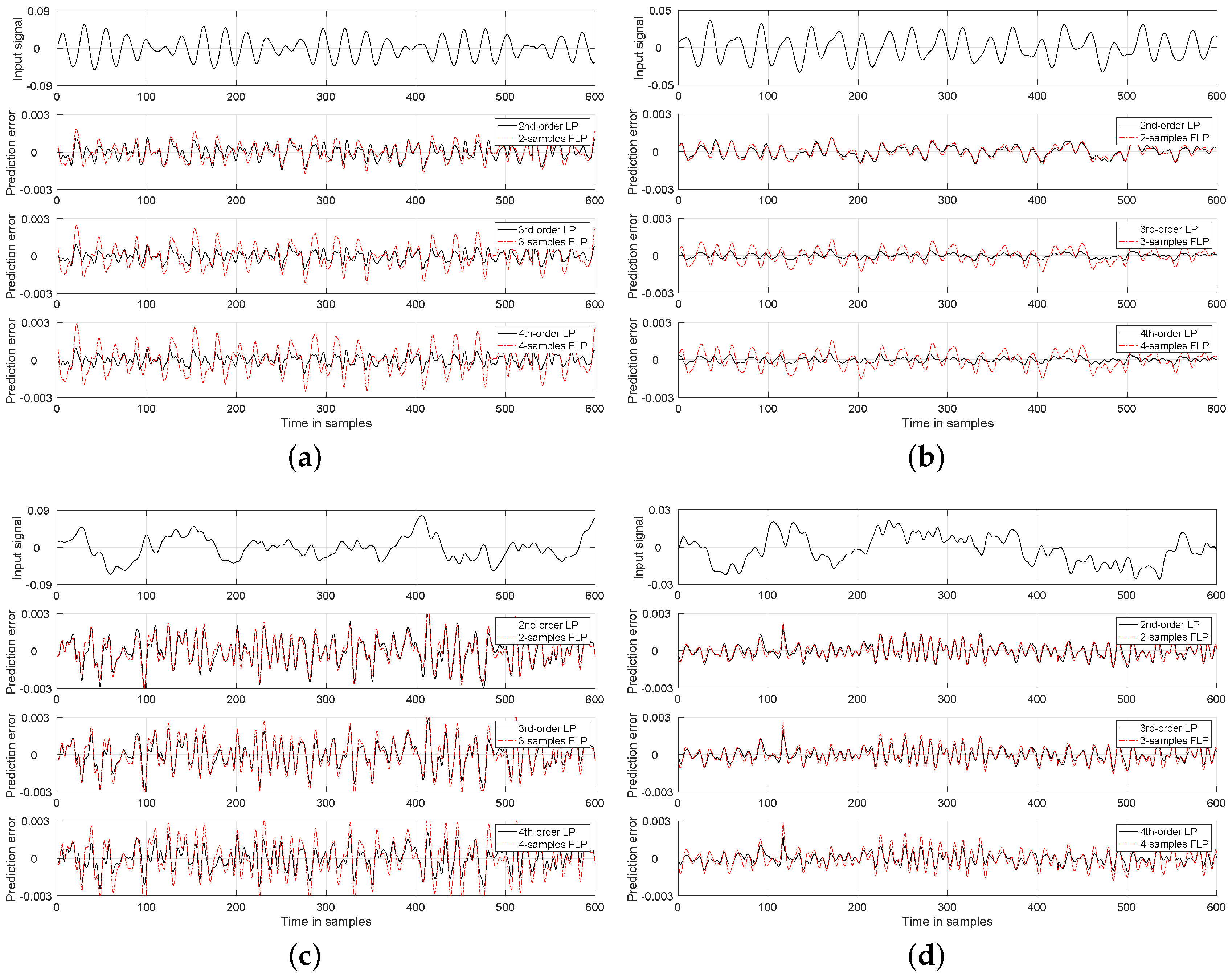
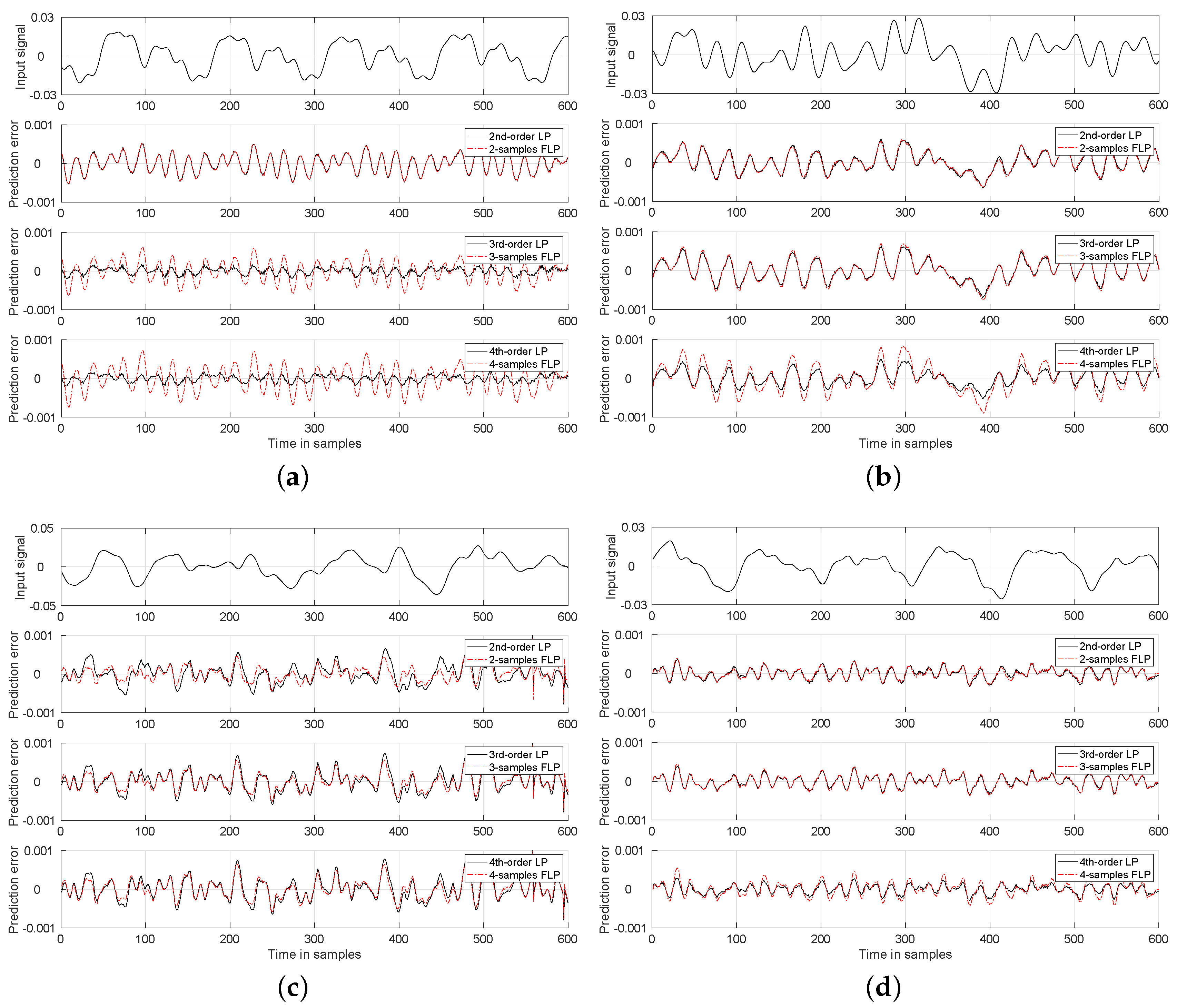
4. Numerical Results and Discussion

The proposed FLP with “restricted memory” given in Equation (10) with the memory of two (Equation (14)), three (Equation (17)) and four samples (Equation (19)) was compared to conventional low-order LP using the same signal history. Experiments were performed using two test signals: the three-note chords composed of randomly chosen notes (MAPS–RAND subset), usual three-notes Western musical chords (MAPS–UCHO subset), and two musical signals: piano recordings (MAPS–MUS subset) and orchestra recordings (Orchset). The signals belonging to one recording condition (studio, jazz club, church, or concert hall) of the particular dataset were concatenated to one signal prior to applying either LP or FLP.

The prediction gain (PG) served as the predictor performance measure, defined as the ratio between the variance of the input signal and the variance of the prediction error measured in decibels:

$$PG\left(dB\right)=10{log}_{10}\frac{{{\sigma }_{\mathbf{x}}}^2}{{{\sigma }_{{\mathbf{e}}_p}}^2}.$$

(21)

The smaller is the error generated by the predictor, the higher is the gain [29].

Experiments

The results for the randomly generated chords (MAPS–RAND subset) for different recording conditions (studio, jazz club, church, and concert hall) using four low-order LP models (first-order, second-order, third-order and fourth-order) and FLP models with the two-sample, three-sample and four-sample memory are presented in

Table 1. Prediction gain (dB) for the chords composed of three randomly chosen notes (MAPS–RAND subset).

			MAPS–RAND
			Studio	Jazz	Church	Concert
120 ms	LP	First-order	17.41	17.53	19.10	15.48
		Second-order	23.94	23.91	26.25	22.51
		Third-order	24.85	24.52	26.89	23.55
		Fourth-order	25.25	24.79	27.15	23.96
	FLP	Two-sample memory	23.40	23.36	25.82	22.14
		Three-sample memory	23.41	23.68	26.02	22.01
		Four-sample memory	23.11	25.06	25.88	21.63
60 ms	LP	First-order	17.15	17.35	18.90	15.23
		Second-order	22.90	22.82	25.15	21.43
		Third-order	23.51	23.42	25.70	22.14
		Fourth-order	23.85	23.66	25.93	22.51
	FLP	Two-sample memory	22.32	22.25	24.71	21.07
		Three-sample memory	22.47	22.66	25.01	21.08
		Four-sample memory	22.28	22.73	24.96	20.81
10 ms	LP	First-order	16.35	16.58	18.13	14.65
		Second-order	19.82	19.95	21.65	18.86
		Third-order	20.28	20.48	22.19	19.29
		Fourth-order	20.46	20.68	22.38	19.50
	FLP	Two-sample memory	19.30	19.37	21.22	18.50
		Three-sample memory	19.74	19.96	21.78	18.80
		Four-sample memory	19.81	20.17	21.94	18.76

. The results show that the first-order LP is inappropriate; however, increasing the prediction-order beyond the second-order LP is not necessary, as it does not bring significant improvement. Similar behavior can be observed for FLP models, where the best performing model is the one with the two-sample memory. For the frames having 120 ms length, its performance is only slightly lower than the performance of the second-order LP, albeit obtained using only one predictor coefficient (note that the second-order LP that also uses the memory of two samples, requires the optimization of two predictor coefficients). By decreasing the frame length, the performance of both LP and FLP decrease, but with FLP approaching LP for the memory of three and four samples. Note that the results for FLP with the memory of three and four samples were obtained using two and three predictor coefficients less than in the case of the third-order and fourth-order LP.

The prediction results for the chords composed of three randomly chosen notes from the MAPS–RAND subset are also presented in Figure 1, where the prediction error using the second-order, third-order and fourth-order LP (black solid line) is compared to the prediction error obtained using the FLP model with two-sample, three-sample and four-sample memory (red dot-dashed line). Ten characteristic frames with the length of 60 ms are shown in the figure. The results confirm that the performance of the second-order LP and the FLP with two-sample memory is comparable for the signals recorded under different conditions (studio, jazz club, church, and concert hall), and the difference between the prediction error of the LP and FLP models is generally increasing with the length of the used memory.

Similar behavior as in case of randomly generated chords can be observed when using usual three-notes Western musical chords (MAPS–UCHO subset). Again, the performance of FLP with two-sample memory is comparable to the second-order LP for all frames, although FLP is using one coefficient less (see

Table 2. Prediction gain (dB) for the usual Western music three-notes chords (MAPS–UCHO subset).

			MAPS–UCHO
			Studio	Jazz	Church	Concert
120 ms	LP	First-order	17.03	18.54	18.74	17.44
		Second-order	24.51	25.75	26.62	25.22
		Third-order	25.25	26.29	27.12	26.02
		Fourth-order	25.61	26.52	27.34	26.39
	FLP	Two-sample memory	23.95	25.08	26.29	24.92
		Three-sample memory	23.90	25.44	26.46	24.78
		Four-sample memory	23.57	25.47	26.29	24.37
60 ms	LP	First-order	16.83	18.37	18.53	17.15
		Second-order	23.53	24.58	25.42	24.07
		Third-order	24.04	25.10	25.91	24.62
		Fourth-order	24.32	25.29	26.08	24.93
	FLP	Two-sample memory	22.97	23.89	25.07	23.76
		Three-sample memory	23.05	24.36	25.36	23.76
		Four-sample memory	22.82	24.47	25.30	23.46
10 ms	LP	First-order	16.07	17.46	17.71	16.38
		Second-order	20.44	21.15	21.77	20.85
		Third-order	20.87	21.74	22.32	21.29
		Fourth-order	21.01	21.93	22.49	21.45
	FLP	Two-sample memory	19.95	20.51	21.45	20.57
		Three-sample memory	20.34	21.15	21.99	20.90
		Four-sample memory	20.37	21.42	22.14	20.88

).

Ten characteristic frames with the length of 60 ms are shown in Figure 2 for the MAPS–UCHO subset, where the prediction error using the second-order, third-order and fourth-order LP (black solid line) is compared to the prediction error obtained using the FLP model with two-sample, three-sample and four-sample memory (red dot-dashed line). The results confirm that the performance of the second-order LP and the FLP with two-sample memory is comparable for the signals recorded under different conditions (studio, jazz club, church, and concert hall), and also that the difference between the prediction errors of the LP and FLP models is increasing with the length of the used memory.

The results for the piano music excerpts using MAPS–MUS subset are also presented for three different frame sizes, i.e., 10 ms, 60 ms and 120 ms (see

Table 3. Prediction gain (dB) for musical signal of classical music pieces played by piano (MAPS–MUS subset) and the classical music pieces performed by orchestra (Orchset dataset).

			MAPS–MUS				Orchset
			Studio	Jazz	Church	Concert
120 ms	LP	First-order	20.54	22.13	21.90	19.60	18.12
		Second-order	31.60	34.04	32.95	30.21	26.82
		Third-order	32.36	34.52	33.51	31.24	27.94
		Fourth-order	32.86	34.75	33.78	31.74	28.15
	FLP	Two-sample memory	31.59	34.02	32.94	30.18	26.70
		Three-sample memory	31.20	34.25	32.98	29.69	26.03
		Four-sample memory	30.55	33.98	32.65	28.96	25.29
60 ms	LP	First-order	20.49	22.00	21.79	19.58	18.08
		Second-order	30.27	32.05	31.28	29.10	26.18
		Third-order	30.81	32.63	31.87	29.82	26.99
		Fourth-order	31.17	32.80	32.07	30.22	27.18
	FLP	Two-sample memory	30.25	32.04	31.26	29.08	26.09
		Three-sample memory	30.14	32.56	31.57	28.83	25.56
		Four-sample memory	29.66	32.44	31.39	28.25	24.91
10 ms	LP	First-order	19.68	20.94	20.77	18.90	17.53
		Second-order	25.18	25.92	25.66	24.60	23.01
		Third-order	25.75	26.75	26.40	25.15	23.37
		Fourth-order	25.92	27.01	26.62	25.35	23.49
	FLP	Two-sample memory	25.17	25.92	25.66	24.57	23.00
		Three-sample memory	25.70	26.74	26.39	24.97	22.93
		Four-sample memory	25.64	27.00	26.52	24.81	22.62

). For shorter frames (10 ms), the performance of FLP is always comparable to the performance of the corresponding LP that uses the same signal memory. For longer frames, PG of FLP is comparable to PG of the corresponding LP for jazz club and church recording conditions, while the performance deteriorates by 1–2 dB only for FLP with the memory of three and four samples for studio and concert recording conditions, suggesting that FLP is better suited for signals recorded in reverberant or non-ideal acoustical conditions. Note that FLP always uses only one predictor coefficient, regardless of the signal memory used for prediction. For example, for the FLP with the four-sample memory, comparable performance is obtained to the corresponding fourth-order LP, but with three predictor coefficients less that need to be optimized. This can lead to substantial savings in bit rate, as predictor coefficients need to be encoded and transferred to receiver end. Furthermore, note that better performance is obtained using longer frames for both LP and FLP; hence, more frequent coefficient update does not bring any improvement.

The last experiment was performed using the orchestra music excerpts from the Orchset dataset. Since LP models are, in general, known to perform well on piano music, we tested the performance of our model on a more challenging music signal played by the orchestra (see Table 3). The performance of FLP in comparison to LP is lower than in piano music; however, the model with two-sample memory is still comparable to the corresponding second-order LP for all frame lengths. Third- and fourth-order LP models perform better than FLP at the expense of two and three additional coefficients, respectively.

When evaluating the prediction error in case of using musical signals from the MAPS–MUS subset (see Figure 3) under the same recording conditions as in previous experiments (e.g., studio, jazz club, church, and concert hall), an interesting observation can be made, i.e., the difference between the prediction error of the LP and FLP models is not increasing that significantly with the length of the used memory (especially for the jazz club and church recording conditions), as was the case of using signals representing chords. Furthermore, it is obvious that the second-order LP and the FLP with two-sample memory for the shown signals perform at the same level for all four recording conditions. Similar behavior is present in the case of using orchestra music excerpts from the Orchset dataset (see Figure 4). Please note that, in Figure 3 and Figure 4, again ten characteristic frames with the length of 60 ms are shown, and that the prediction error using the second-order, third-order and fourth-order LP (black solid line) is compared to the prediction error obtained using the FLP model with two-sample, three-sample and four-sample memory (red dot-dashed line).

Here, it should be emphasized that LP and FLP models always use the same number of previous samples (two, three and four) that allows a fair comparison. Furthermore, it is important to emphasize that all FLP models show comparable performance in comparison to LP models, even though they use only two coefficients, i.e., one predictor coefficient a and one order of fractional derivative $\alpha$, in comparison to LP models that use two, three and four predictor coefficients (based on the order of the LP predictor). Moreover, the order of fractional differentiation $\alpha$ does not have to be computed or optimized. It might be estimated as the inverse of the predictor memory, as previously shown in [21,22], resulting in only one FLP coefficient that has to be encoded and transmitted. This makes the proposed FLP significantly more efficient than LP.

5. Conclusions

Fractional linear prediction with “restricted memory” that uses two, three, and four previous samples, respectively, for audio signal prediction is discussed in this work and the closed-form expressions for the FLP predictor coefficient are derived. Two datasets were used for the experiments to test the performance of the model and compare it to linear prediction, i.e., MAPS dataset, which contains chords composed of randomly chosen notes, usual chords in Western music, and piano music excerpts; and Orchset dataset, which contains music excerpts, extracted from symphonies, ballets and other classical musical forms, and interpreted by symphonic orchestras.

Using the same number of previous samples for prediction, the results show that FLP is better suited for prediction of audio signal than the conventional low-order LP models, since it provides comparable performance, even though it uses less parameters (one predictor coefficients and one order of fractional derivative). Furthermore, the order of fractional derivative does not have to be optimized and can be assumed as the inverse of the memory length of the FLP model, making it even more efficient in comparison to LP model, where the number of predictor coefficients is always equal to the predictor order. For example, FLP with the memory of four samples requires only one predictor coefficient, whereas the corresponding fourth-order LP requires four predictor coefficients, at similar performance. Therefore, substantial savings in transmission costs are possible.

References

1. Purnhagen, H.; Meine, N. HILN–The MPEG-4 Parametric Audio Coding Tools. In Proceedings of the 2000 IEEE International Symposium on Circuits and Systems. Emerging Technologies for the 21st Century, Geneva, Switzerland, 28–31 May 2000; Volume 3, pp. 201–204. [Google Scholar]
2. Marchand, S.; Strandh, R. InSpect and ReSpect: Spectral Modeling, Analysis and Real-Time Synthesis Software Tools for Researchers and Composers. In Proceedings of the Int. Computer Music Conference (ICMC 1999), Beijing, China, 22–27 October 1999; pp. 341–344. [Google Scholar]
3. Lagrange, M.; Marchand, S. Long Interpolation of Audio Signals Using Linear Prediction in Sinusoidal Modeling. J. Audio Eng. Soc. 2005, 53, 891–905. [Google Scholar]
4. Thompson, W.F. Music, Thought, and Feeling: Understanding the Psychology of Music; Oxford University Press: Oxford, UK; New York, NY, USA, 2008. [Google Scholar]
5. Atal, B.S. The History of Linear Prediction. IEEE Signal Process. Mag. 2006, 23, 154–161. [Google Scholar] [CrossRef]
6. Benesty, J.; Chen, J.; Huang, Y. Linear Prediction. In Springer Handbook of Speech Processing; Benesty, J., Sondhi, M.M., Huang, Y., Eds.; Springer: Berlin, Germany, 2007; Chapter 7; pp. 121–133. [Google Scholar]
7. Vaidyanathan, P.P. The Theory of Linear Prediction; Synthesis Lectures on Signal Processing; Morgan & Claypool: San Rafael, CA, USA, 2008. [Google Scholar]
8. van Waterschoot, T.; Moonen, M. Comparison of linear prediction models for audio signals. EURASIP J. Audio Speech Music Process. 2009, 2008. [Google Scholar] [CrossRef]
9. Harma, A.; Laine, U.K. A comparison of warped and conventional linear predictive coding. IEEE Trans. Speech Audio Process. 2001, 9, 579–588. [Google Scholar] [CrossRef]
10. Deriche, M.; Ning, D. A novel audio coding scheme using warped linear prediction model and the discrete wavelet transform. IEEE Trans. Audio Speech Lang. Process. 2006, 14, 2039–2048. [Google Scholar] [CrossRef]
11. Van Waterschoot, T.; Rombouts, G.; Verhoeve, P.; Moonen, M. Double-talk-robust prediction error identification algorithms for acoustic echo cancellation. IEEE Trans. Signal Process. 2007, 55, 846–858. [Google Scholar] [CrossRef]
12. Mahkonen, K.; Eronen, A.; Virtanen, T.; Helander, E.; Popa, V.; Leppanen, J.; Curcio, I.D. Music dereverberation by spectral linear prediction in live recordings. In Proceedings of the 16th Int. Conference on Digital Audio Effects (DAFx-13), Maynooth, Ireland, 2–6 September 2013; pp. 1–4. [Google Scholar]
13. Grama, L.; Rusu, C. Audio signal classification using Linear Predictive Coding and Random Forests, Bucharest, Romania. In Proceedings of the International Conference on Speech Technology and Human-Computer Dialogue (SpeD 2017), Bucharest, Romania, 6–9 July 2017. [Google Scholar]
14. Glover, J.; Lazzarini, V.; Timoney, J. Real-time detection of musical onsets with linear prediction and sinusoidal modeling. EURASIP J. Adv. Signal Process. 2011, 2011, 68. [Google Scholar] [CrossRef] [Green Version]
15. Marchi, E.; Ferroni, G.; Eyben, F.; Gabrielli, L.; Squartini, S.; Schuller, B. Multi-resolution linear prediction based features for audio onset detection with bidirectional LSTM neural networks. In Proceedings of the IEEE International Conference on Acoustic, Speech and Signal Processing (ICASSP 2014), Florence, Italy, 4–9 May 2014; pp. 2183–2187. [Google Scholar]
16. Skovranek, T.; Despotovic, V. Signal Prediction using Fractional Derivative Models. In Handbook of Fractional Calculus with Applications; Baleanu, D., Lopes, A.M., Eds.; Walter de Gruyter GmbH: Berlin/Munich, Germany; Boston, MA, USA, 2019; Volume 8, Chapter 7; pp. 179–206. [Google Scholar]
17. Joshia, V.; Pachori, R.B.; Vijesh, A. Classification of ictal and seizure-free EEG signals using fractional linear prediction. Biomed. Signal Process. Control 2014, 9, 1–5. [Google Scholar] [CrossRef]
18. Talbi, M.L.; Ravier, P. Detection of PVC in ECG Signals Using Fractional Linear Prediction. Biomed. Signal Process. Control 2016, 23, 42–51. [Google Scholar] [CrossRef]
19. Assaleh, K.; Ahmad, W.M. Modeling of Speech Signals Using Fractional Calculus. In Proceedings of the 9th International Symposium on Signal Processing and Its Applications (ISSPA’07), Sharjah, UAE, 12–15 February 2007; pp. 1–4. [Google Scholar]
20. Despotovic, V.; Skovranek, T. Fractional-order Speech Prediction. In Proceedings of the International Conference on Fractional Differentiation and its Applications (ICFDA’16), Novi Sad, Serbia, 18–20 July 2016; pp. 124–127. [Google Scholar]
21. Despotovic, V.; Skovranek, T.; Peric, Z. One-parameter fractional linear prediction. Comput. Electr. Eng. Spec. Issue Signal Process. 2018, 69, 158–170. [Google Scholar] [CrossRef]
22. Skovranek, T.; Despotovic, V.; Peric, Z. Optimal Fractional Linear Prediction With Restricted Memory. IEEE Signal Process. Lett. 2019, 26, 760–764. [Google Scholar] [CrossRef]
23. Podlubny, I. Fractional Differential Equations; Academic Press: San Diego, CA, USA, 1999. [Google Scholar]
24. Emiya, V.; Badeau, R.; David, B. Multipitch estimation of piano sounds using a new probabilistic spectral smoothness principle. IEEE Trans. Audio Speech Lang. Process. 2010, 18, 1643–1654. [Google Scholar] [CrossRef]
25. Emiya, V. Transcription Automatique de la Musique de Piano. Ph.D. Thesis, Telecom ParisTech, Paris, France, October 2008. [Google Scholar]
26. Bosch, J.; Marxer, R.; Gomez, E. Evaluation and Combination of Pitch Estimation Methods for Melody Extraction in Symphonic Classical Music. J. New Music Res. 2016, 45, 101–117. [Google Scholar] [CrossRef]
27. Driedger, J.; Mueller, M. A Review of Time-Scale Modification of Music Signals. Appl. Sci. 2016, 6, 57. [Google Scholar] [CrossRef]
28. Theodoridis, S.; Koutroumbas, K. Pattern Recognition, 4th ed.; Academic Press: San Diego, CA, USA, 2008. [Google Scholar]
29. Chu, W.C. Speech Coding Algorithms: Foundation and Evolution of Standardized Coders; John Wiley & Sons: Hoboken, NJ, USA, 2003. [Google Scholar]
Figure 1. The prediction error results for the random chords (MAPS–RAND) for second-order, third-order and fourth-order LP and the FLP with the two-sample, three-sample, and four-sample memory: (a) studio recording; (b) jazz club recording; (c) church recording; and (d) concert hall recording.
Mathematics 07 00580 g001
Figure 2. The prediction error results for the three-notes chords (MAPS–UCHO) for second-order, third-order and fourth-order LP and the FLP with the two-sample, three-sample, and four-sample memory: (a) studio recording; (b) jazz club recording; (c) church recording; and (d) concert hall recording.
Mathematics 07 00580 g002
Figure 3. The prediction error results for the musical signals (MAPS–MUS) for second-order, third-order and fourth-order LP and the FLP with the two-sample, three-sample, and four-sample memory: (a) studio recording; (b) jazz club recording; (c) church recording; and (d) concert hall recording.
Mathematics 07 00580 g003
Figure 4. The prediction error results for the musical signal (Strauss–BlueDanube–ex1, from the Orchset) for second-order, third-order and fourth-order LP and the FLP with the two-sample, three-sample, and four-sample memory.
Mathematics 07 00580 g004