Reliability Analysis of the Bijective Connection Networks for Components

Abstract

Connectivity is a critical parameter that can measure the reliability of networks. Let $Q\subseteq V\left(G\right)$ be a vertex set. If $G-Q$ is disconnected and every component of $G-Q$ contains at least $k+1$ vertices, then Q is an extra-cut. The number of vertices in the smallest extra-cut is the extraconnectivity ${\kappa }_k\left(G\right)$. Suppose $\omega \left(G\right)$ is the number of components of G and $W\subseteq V\left(G\right)$; if $\omega (G-W)\ge t$, then w is a t-component cut of G. The number of vertices in the least t-component cut is the t-component connectivity $c{\kappa }_t\left(G\right)$ of G. The t-component edge connectivity $c{\lambda }_t\left(G\right)$ is defined similarly. In this note, we study the BC networks and obtain the t-component (edge) connectivity of bijective connection networks for some t.

1. Introduction

Multiprocessor systems have many advantages over their uniprocessor counterparts, such as high performance and reliability, better reconfigurability, and scalability. With the development of VLSItechnology and software technology, multiprocessor systems with hundreds of thousands of processors have become available. With the continuous increase in the size of multiprocessor systems, the complexity of a system can adversely affect its fault tolerance and reliability. For the design and maintenance purpose of multiprocessor systems, appropriate measures of reliability should be found.

A graph $G=(V,E)$ can simulate a network. The edges can represent links between the nodes, and the vertices can represent nodes that are processors or stations. Reliability is the essential consideration in network design [1,2]. For a connected graph G, the connectivity $\kappa \left(G\right)$ is defined as the minimum number k of vertices that can be removed to reduce the graph connectivity or leave only one vertex. For the reliability of networks, connectivity is worst for most measures. To compensate for this shortcoming, it seems reasonable to generalize the notion of classical connectivity by imposing some conditions or restrictions on the components of $G-F$, where F denotes faulty processors/links. Hence, many parameters that can measure the reliability of multiprocessor systems have been proposed. Suppose $S_1\subseteq V\left(G\right)$; if $\omega (G-S_1)\ge t$, then $S_1$ is a t-component cut of G. The number of vertices in the least t-component cut is the t-component connectivity $c{\kappa }_t\left(G\right)$ of G. Correspondingly, the t-component edge connectivity $c{\lambda }_t\left(G\right)$ is obtained. The t-component (edge) connectivity was proposed in [3,4] independently. Fábrega et al. proposed extraconnectivity in [5]. Let $F_1\subseteq V\left(G\right)$ be a vertex set. If $G-F_1$ is disconnected and every component of $G-F_1$ contains at least $p+1$ vertices, then $F_1$ is an extra-cut. The number of vertices in the smallest extra-cut is the extraconnectivity ${\kappa }_p\left(G\right)$.

Suppose $G=(V,E)$ is a connected graph, $N_G\left(w\right)=\{u:wu\in E\}$ (simply $N\left(w\right)$), $E\left(w\right)=\{e:$e is an edge, and w is an end of e}.

Q is a subset of V; $G\left[Q\right]$ is the subgraph induced by the vertices in Q, $N_G\left(Q\right)={\cup }_{v\in Q}N\left(v\right)-Q,N_G\left[Q\right]=N_G\left(Q\right)\cup Q$; $G-Q$ is the subgraph of G that is induced by the vertices of $V-Q$. If $p,q\in V$, then $d(p,q)$ is the number of edges of the shortest $(p,q)$-path. For $P,Q\subset V$, the edge set $[P,Q]=\{e:e=wz\in E,w\in P,z\in Q\}$. We follow [6] for terminology and notation. We only consider simple, finite, and undirected graphs.

Definition 1. 

BC networks:The one-dimensional bijective connection network $X_1$ is the complete graph $K_2$. Let $L_1=\left\{X_1\right\}$ and G be an n-dimensional BC graph. Suppose $L_n=\{G:G$ is an n-dimensional bijective connection graph}. An n-dimensional BC graph G can be defined recursively:

(1) 

For two non-empty subsets $V_1,V_2\subset V\left(G\right)$, $V\left(G\right)=V_1\cup V_2$;

(2) 

An edge set $Q\subset E\left(G\right)$, Q is a perfect matching between $V_1$ and $V_2$, $G\left[V_1\right],G\left[V_2\right]\in L_{n-1}$.

In the following, we denote $X_n$ an n-dimensional BC network. The n-dimensional BC network $X_n$ with $2^n$ vertices and $n{2}^{n-1}$ edges was introduced by Fan et al. [7]. An n-dimensional BC graph $X_n$ is n regular Hamilton-connected. BC graphs contain most of the variants of the hypercube: hypercube, crossed cube, twisted cube, locally-twisted cube, and so on. We can see that $L_1=\left\{K_2\right\}$, $L_2=\left\{C_4\right\}$, $L_3=\{Q_3,C{Q}_3,T{Q}_3,LT{Q}_3\}$, where $C_4$ is a four-cycle, $Q_3$ is a three-dimensional hypercube, $C{Q}_3$ is a three-dimensional crossed cube, $T{Q}_3$ is a three-dimensional twisted cube, and $LT{Q}_3$ is a three-dimensional locally-twisted cube. $T{Q}_3$ and $LT{Q}_3$ are isomorphs of $C{Q}_3$.

According to the definition, every vertex of $X_{n-1}^0$ has only one neighbor in $X_{n-1}^1$, and every vertex of $X_{n-1}^1$ also has only one neighbor in $X_{n-1}^0$. Because $X_n$ can be obtained by putting a perfect matching W between $X_{n-1}^0$ and $X_{n-1}^1$, $X_n$ can be viewed as $G(X_{n-1}^0,X_{n-1}^1,W)$ or $X_{n-1}^0\odot X_{n-1}^1$. Suppose $w\in V\left(X_n\right),e_W\left(w\right)$ is the edge incident to w in W.

The BC graphs are an attractive alternative to hypercubes $Q_n$. For more references about BC networks, see [8,9,10,11,12,13]. For more references about component connectivity, see [14,15,16].

In this work, we get that:

(1)

Suppose $(n\ge 2)$; $c{\kappa }_2\left(X_n\right)=n$.

(2)

Suppose $(n\ge 3)$; $c{\kappa }_3\left(X_n\right)=2n-2$.

(3)

Suppose $(n\ge 2)$; $c{\lambda }_2\left(X_n\right)=n$.

(4)

Suppose $(n\ge 2)$; $c{\lambda }_3\left(X_n\right)=2n-1$.

(5)

Suppose $(n\ge 2)$; $c{\lambda }_4\left(X_n\right)=3n-2$.

2. Properties of BC Networks

The BC networks $X_n$ has an important property as follows.

Lemma 1 

([11]). Let $p,q\in V\left(X_n\right)(n\ge 2)$ be any two vertices. Then, $\left|N\right(p)\cap N(q\left)\right|\le 2$.

Corollary 1.

Suppose that $p,q\in V\left(X_n\right)(n\ge 2)$ are any two vertices. Then,

(1) 

if $d(p,q)$ is two, then $\left|N\right(p)\cap N(q\left)\right|\le 2$;

(2) 

if $d(p,q)\ne 2$, then $\left|N\right(p)\cap N(q\left)\right|=0$.

From Lemma 1, we can see that the girth of $X_n$ is $g\left(X_n\right)=4(n>1)$. By the definition of $X_n$, we obtain:

Lemma 2.

Suppose that $p,q\in V\left(X_n\right)(n\ge 2)$ are any two vertices such that $\left|N\right(p)\cap N(q\left)\right|=\{w,z\}$.

(1) 

If $p\in V\left(X_{n-1}^0\right),q\in V\left(X_{n-1}^1\right)$, then $w\in X_{n-1}^0$ and $z\in X_{n-1}^1$.

(2) 

If $p,q\in V\left(X_{n-1}^0\right)$ or $V\left(X_{n-1}^1\right)$, then $\{w,z\}\subseteq X_{n-1}^0$ or $\{w,z\}\subseteq X_{n-1}^1$.

Lemma 3

([7]). If $n\ge 2$, then $\kappa \left(X_n\right)=\lambda \left(X_n\right)=n$.

Theorem 1.

If $n\ge 2$, $c{\kappa }_2\left(X_n\right)=\kappa \left(X_n\right)=n$.

Theorem 2.

Suppose $(n\ge 3)$, $c{\kappa }_3\left(X_n\right)=2n-2$.

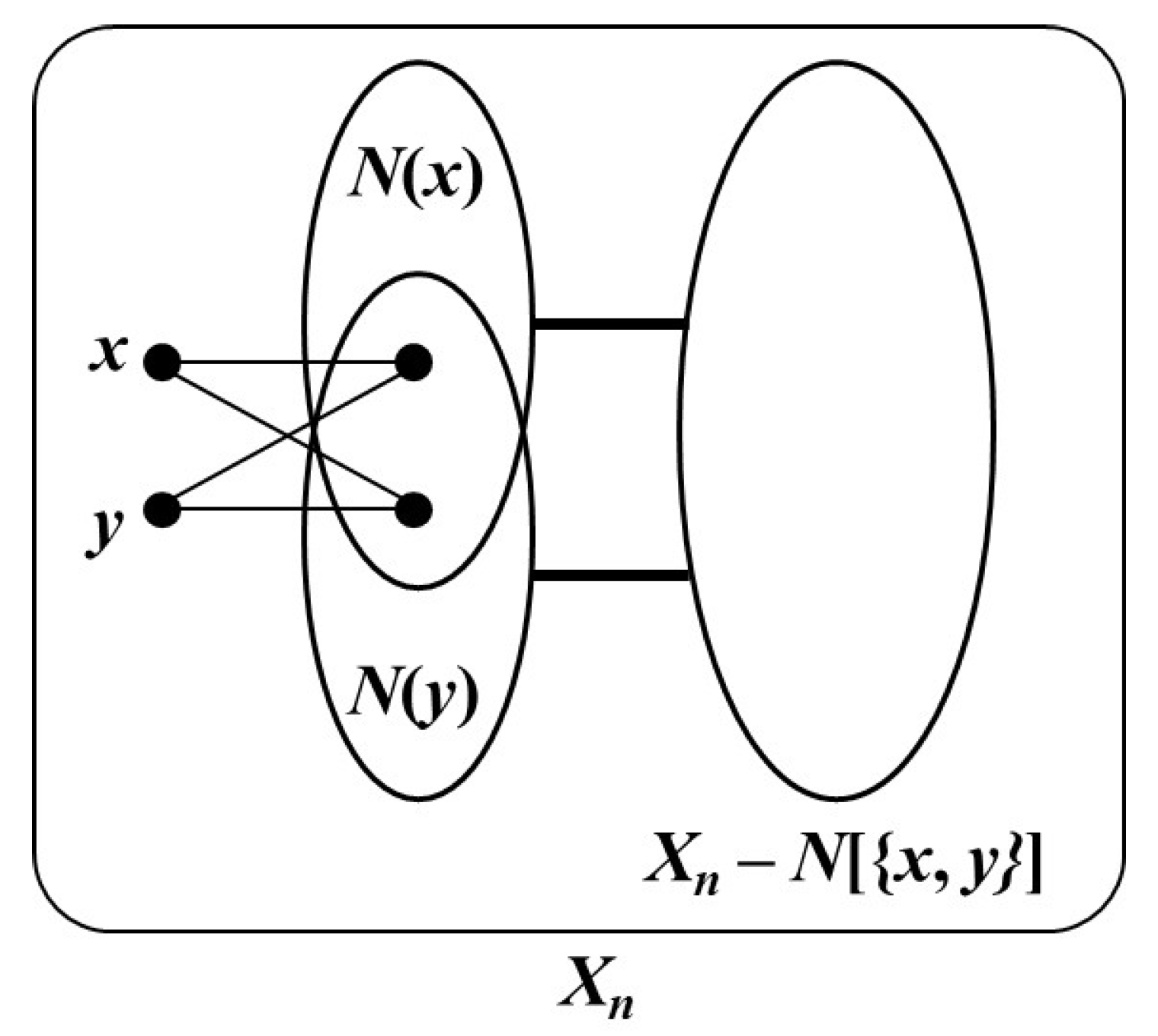
Proof. 

In a cycle $C_4$, take $x,y$ with $\left|N\right(x)\cap N(y\left)\right|=2,xy\notin E$. Then, $\omega (X_n-N\left(\{x,y\}\right))\ge 3$ (see Figure 1) and $\left|N\right(\{x,y\}\left)\right|=2n-2$. Hence, $c{\kappa }_3\left(X_n\right)\le 2n-2$.

Figure 1. Illustration of $X_n-N\left(\{x,y\}\right)$.

We will show $c{\kappa }_3\left(X_n\right)\ge 2n-2$ by induction; this is right for $n=3$. Hence, let $n\ge 4$. Suppose that the case of $n\le k-1$ is true. Set $n=k$.

By contradiction, suppose $Q\subseteq V\left(X_n\right)$ and $\left|Q\right|\le 2n-3$. Furthermore, $\omega (X_n-Q)\ge 3$, say $G_1,G_2$ and $G_3$. We have $|Q\cap V(X_{n-1}^0\left)\right|\le n-2$ or $|Q\cap V(X_{n-1}^1\left)\right|\le n-2$. We set $|Q\cap V(X_{n-1}^0\left)\right|\le n-2$ by symmetry. Hence, $X_{n-1}^0-Q$ must be connected.

If $\omega (X_{n-1}^1-Q)\ge 3$, then $|Q\cap V(X_{n-1}^1\left)\right|\ge 2n-4$ by the inductive hypothesis, and $|Q\cap V(X_{n-1}^0\left)\right|\le 1$. Since every vertex of $X_{n-1}^1$ has one neighbor in $X_{n-1}^0$, at most one vertex of $X_{n-1}^1-Q$ does not have neighbors in $X_{n-1}^0-Q$. Hence, $\omega (X_n-Q)\le 2$, a contradiction.

Hence, $\omega (X_{n-1}^1-Q)\le 2$. At most one connected component of $X_{n-1}^1-Q$ is not connected to $X_{n-1}^0-Q$. Then, $\omega (X_n-Q)\le 2$, a contradiction again. □

Lemma 4.

Let $w\in V\left(X_n\right)(n\ge 3)$ be an any vertex. The connectivity $\kappa (X_n-N\left[w\right])$ is $n-2$.

Proof. 

Since $\delta (X_n-N\left[w\right])=n-2$, $\kappa (X_n-N\left[w\right])\le n-2$. We need to prove $\kappa (X_n-N\left[w\right])\ge n-2$. The case of $n=3$ is true. Set $n\ge 4$ and $w\in V\left(X_{n-1}^0\right)$.

By contradiction, suppose $K\subseteq V\left(X_n\right)$ with $\left|K\right|\le n-3$. Next, it will be proven that $X_n-N\left[w\right]-K$ is connected. Since $\kappa \left(X_{n-1}\right)=n-1$, $X_{n-1}^1-N_{X_{n-1}^1}\left(w\right)-K$ is connected. By Theorem 4, $c{\kappa }_3\left(X_{n-1}\right)=2n-4>n-3(n\ge 4)$, then $\omega (X_{n-1}^0-N_{X_{n-1}^0}\left(w\right))=2$: one component is the vertex w, and the other component is $G_1=X_{n-1}^0-N_{X_{n-1}^0}\left(w\right)-w$. However, $|X_{n-1}^0-N_{X_{n-1}^0}\left[w\right]|=2^{n-1}-n>n-3$ for $(n\ge 4)$, and at least one vertex of $G_1$ is connected to $X_{n-1}^1-N_{X_{n-1}^1}\left(w\right)-K$. Then, $X_n-N\left[w\right]-K$ is connected, and this contradicts the hypothesis. □

Lemma 5.

Suppose $n\ge 3$, then ${\kappa }_1\left(X_n\right)=2n-2$.

Proof. 

Pick an edge $e=wz$. Therefore, $X_n-N\left(\{w,z\}\right)$ is disconnected, and at least two vertices are contained in every connected component. That is ${\kappa }_1\left(X_n\right)\le 2n-2$.

It suffices to show ${\kappa }_1\left(X_n\right)\ge 2n-2$ by induction. The case of $n=3$ is true. Assume that $n\ge 4$, and this is right when $n<k$. This will be proven for $n=k$.

By contradiction, suppose $R\subseteq V\left(X_n\right)$ with $\left|R\right|\le 2n-3$. We will show that $X_n-R$ is connected or $X_n-R$ contains an isolated vertex. We suppose $|R\cap V(X_{n-1}^0\left)\right|\le n-2$ by symmetry. Then, $X_{n-1}^0-R$ is connected.

If each connected component of $X_{n-1}^1-R$ contains more than one vertex, according to the inductive hypothesis, $|R\cap V(X_{n-1}^1\left)\right|\ge 2n-4$ and $|R\cap V(X_{n-1}^0\left)\right|\le 1$. At most one vertex of $X_{n-1}^1-R$ does not have neighbors in $X_{n-1}^0-R$. Hence, $X_n-R$ is connected.

Suppose $x^{\prime }$ is the isolated vertex of $X_{n-1}^1-R$. Note that $|N_{X_{n-1}^1}\left(x^{\prime }\right)|=n-1$, and by Lemma 4, $\kappa (X_{n-1}^1-N_{X_{n-1}^1}\left[x^{\prime }\right])=n-3$. If $|R\cap V(X_{n-1}^1\left)\right|\ge 2n-4$, then $|R\cap V(X_{n-1}^0\left)\right|\le 1$. Then, $X_n-R$ has an isolated vertex $x^{\prime }$, or $X_n-R$ has an isolated vertex $y^{\prime }$ whose degree is $n-3$ in $X_{n-1}^1-N_{X_{n-1}^1}\left[x^{\prime }\right]$, or $X_{n-1}^1-R$ is connected to $X_{n-1}^0-R$, a contradiction.

Assume $|R\cap V(X_{n-1}^1\left)\right|\le 2n-5$. Since $N_{X_{n-1}^1}\left(x^{\prime }\right)\subseteq R,\kappa (X_{n-1}^1-N_{X_{n-1}^1}\left[x^{\prime }\right])=n-3$, and $|R\cap V\left(X_{n-1}^1\right)-N_{X_{n-1}^1}(x^{\prime })|\le n-4$, $X_{n-1}^1-R-x^{\prime }$ is connected by Lemma 4. However, $2^{n-1}-(n-2)>2n-3(n\ge 4)$, $X_{n-1}^1-R-x^{\prime }$ is connected to $X_{n-1}^0-R$ or $X_n-R$ has an isolated vertex $x^{\prime }$, and this contradicts the hypothesis. □

Theorem 3.

Suppose $n\ge 2$, $c{\lambda }_2\left(X_n\right)=\lambda \left(X_n\right)=n$.

Theorem 4.

Suppose $n\ge 2$, $c{\lambda }_3\left(X_n\right)=2n-1$.

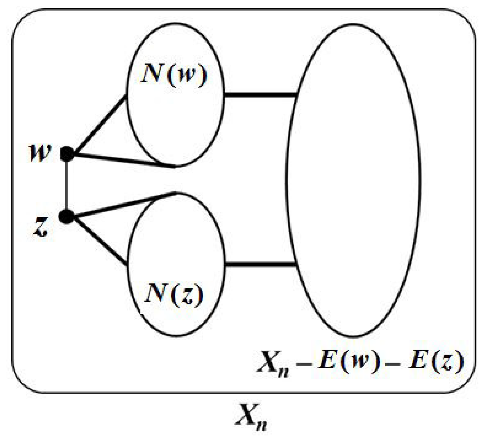
Proof. 

Pick an edge $e=wz$, then $\left|E\right(w)\cup E(z\left)\right|=2n-1$. $\omega (X_n-E\left(w\right)-E\left(z\right))\ge 3$ (see Figure 2). That is, $c{\lambda }_3\left(X_n\right)\le 2n-1$.

Figure 2. Illustration of $X_n-E\left(w\right)-E\left(z\right)$.

Next, we will show that $c{\lambda }_3\left(X_n\right)\ge 2n-1$ by induction. The cases of $n=2,3$ are true. Therefore, we set $n\ge 4$, and this is right for $n<k$. Next, for $n=k$, it will be proven that this is right.

By contradiction, suppose $R\subseteq E\left(X_n\right)$, $\left|R\right|\le 2n-2$, and $X_n-R$ has at least three components. Since $X_n=X_{n-1}^0\odot X_{n-1}^1$, we have $\left|E\right(X_{n-1}^0)\cap R|\le n-1$ or $\left|E\right(X_{n-1}^1)\cap R|\le n-1$, say $\left|E\right(X_{n-1}^0)\cap R|\le n-1$. Note that $\lambda \left(X_{n-1}\right)=n-1$.

Case 1. 

$X_{n-1}^0-R$ is disconnected.

We obtain $\left|E\right(X_{n-1}^0)\cap R|=n-1$ and $\omega (X_{n-1}^0-R)=2$.

If $X_{n-1}^1-R$ is disconnected, then $\left|E\right(X_{n-1}^1)\cap R|=n-1$. That is $[X_{n-1}^0,X_{n-1}^1]\cap R=\varnothing$. However, every vertex of $X_{n-1}^1-R$ has a path to one component of $X_{n-1}^0-R$. Hence, $X_n-R$ has at most two components, and this is a contradiction.

Since $|[X_{n-1}^0,X_{n-1}^1]|=2^{n-1}>n-1(n\ge 4)$, if $X_{n-1}^1-R$ is connected, then $X_{n-1}^1-R$ has a path to one component of $X_{n-1}^0-R$. Hence, $\omega (X_n-R)\le 2$, and this is a contradiction.

Case 2. 

$X_{n-1}^0-R$ is connected.

If $X_{n-1}^1-R$ is connected, then it holds. Assume that $X_{n-1}^1-R$ is not connected. At most one isolated vertex is in $X_{n-1}^1-R$ since $\left|R\right|\le 2n-2$.

If $\omega (X_{n-1}^1-R)\ge 3$, then $\left|E\right(X_{n-1}^1)\cap R|\ge 2n-3$ by the inductive hypothesis. Then, at most one of the components of $X_{n-1}^1-R$ is not connected to $X_{n-1}^0-R$, $\omega (X_n-R)\le 2$, a contradiction.

Therefore, we suppose that $\omega (X_{n-1}^1-R)=2$. However, $2^{n-1}-(2n-2)>0(n\ge 4)$, $\omega (X_n-R)\le 2$, a contradiction. □

Theorem 5.

Suppose $n\ge 2$, then $c{\lambda }_4\left(X_n\right)=3n-2$.

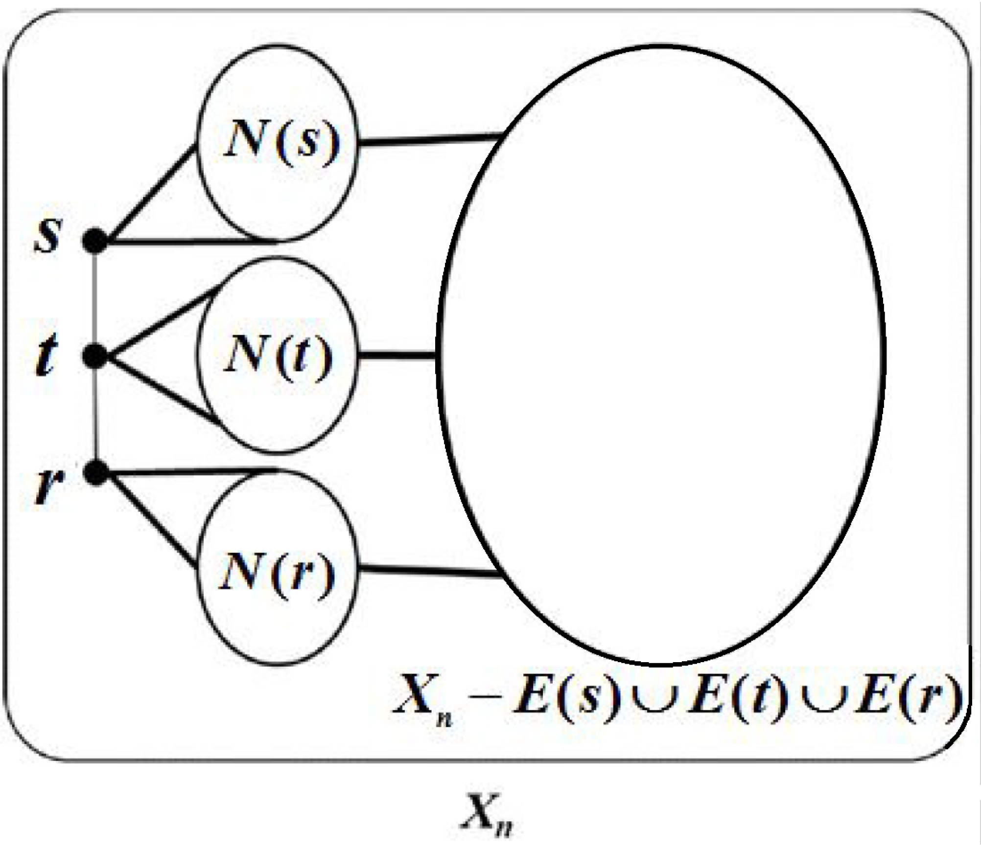
Proof. 

Pick a path $P_3=str$. Then, $\left|E\right(s)\cup E(t)\cup E(r\left)\right|=3n-2$. Then, $\omega (X_n-(E\left(s\right)\cup E\left(t\right)\cup E\left(r\right)))\ge 4$ (see Figure 3). That is, $c{\lambda }_4\left(X_n\right)\le 3n-2$.

Figure 3. Illustration of $X_n-(E\left(s\right)\cup E\left(t\right)\cup E\left(r\right))$.

Next, we will show that $c{\lambda }_4\left(X_n\right)\ge 3n-2$ by induction. The cases of $n=2,3$ are true. Therefore, we suppose $n\ge 4$ and assume all the cases of $n<k$ are true. We will prove that the case of $n=k$ holds.

By contradiction, assume that $U\subseteq E\left(X_n\right)$, $\left|U\right|\le 3n-3$, and $\omega (X_n-U)\ge 4$. Since $X_n=X_{n-1}^0\odot X_{n-1}^1$, we have $|E\left(X_{n-1}^0\right)\cap U|\le \lceil 3n/2\rceil -2$ or $|E\left(X_{n-1}^1\right)\cap U|\le \lceil 3n/2\rceil -2$, say $|E\left(X_{n-1}^0\right)\cap U|\le \lceil 3n/2\rceil -2$. Since $c{\lambda }_3\left(X_{n-1}\right)=2n-3>\lceil 3n/2\rceil -2(n\ge 4)$, $\omega (X_{n-1}^0-U)\le 2$.

Case 1. 

$X_{n-1}^0-U$ is connected.

If $\omega (X_{n-1}^1-U)\ge 4$, then $c{\lambda }_4\left(X_{n-1}\right)\ge 3n-5$ according to the inductive hypothesis. At most two edges need to be deleted again. Because every vertex of $X_{n-1}^1$ has a neighbor in $X_{n-1}^0$ and $|[X_{n-1}^0,X_{n-1}^1]|=2^{n-1}>2(n\ge 4)$, $\omega (X_n-U)\le 3$, a contradiction.

Suppose $\omega (X_{n-1}^1-U)\le 3$. If $n=4$, then $|[X_3^0,X_3^1]|=8<(3n-3)=9$. Assume that $[X_3^0,X_3^1]\subset U$. At most one edge needs to be delete again. Note that $\lambda \left(X_3\right)=3$, and $X_3^1-U$ and $X_3^0-U$ are connected. Hence, $\omega (X_4-U)=2$, a contradiction. Then, $[X_3^0,X_3^1]⊈U$. At least one component of $X_{n-1}^1-U$ is connected to $X_{n-1}^0-U$. Then, $\omega (X_n-U)\le 3$, a contradiction again.

Then, let $n\ge 5$. Because of $|[X_{n-1}^0,X_{n-1}^1]|=2^{n-1}>3n-3(n\ge 5)$, $\omega (X_n-U)\le 3$, a contradiction.

Case 2. 

$\omega (X_{n-1}^0-U)=2$.

Then, $|E\left(X_{n-1}^0\right)\cap U|\ge \lambda \left(X_{n-1}\right)=n-1$ and $\left|E\right(X_{n-1}^1)\cap U|\le 2n-2$. Note that $c{\lambda }_3\left(X_{n-1}\right)=2n-3$.

If $\omega (X_{n-1}^1-U)\ge 3$, then $\left|E\right(X_{n-1}^1)\cap U|\ge 2n-3$ and $\left|E\right(X_{n-1}^0)\cap U|\le n$. However, $\left|\right[X_{n-1}^0,X_{n-1}^1]\cap U|\le 1$ and $2^{n-1}>1(n\ge 4)$, $\omega (X_n-U)\le 3$, a contradiction.

Hence, $\omega (X_{n-1}^1-U)\le 2$. We have $|[X_{n-1}^0,X_{n-1}^1]|=2^{n-1}>3n-3-(n-1)(n\ge 4)$, and $\omega (X_n-U)\le 3$, a contradiction. □