Some q-Rung Picture Fuzzy Dombi Hamy Mean Operators with Their Application to Project Assessment

Abstract

The recently proposed q-rung picture fuzzy set (q-RPFSs) can describe complex fuzzy and uncertain information effectively. The Hamy mean (HM) operator gets good performance in the process of information aggregation due to its ability to capturing the interrelationships among aggregated values. In this study, we extend HM to q-rung picture fuzzy environment, propose novel q-rung picture fuzzy aggregation operators, and demonstrate their application to multi-attribute group decision-making (MAGDM). First of all, on the basis of Dombi t-norm and t-conorm (DTT), we propose novel operational rules of q-rung picture fuzzy numbers (q-RPFNs). Second, we propose some new aggregation operators of q-RPFNs based on the newly-developed operations, i.e., the q-rung picture fuzzy Dombi Hamy mean (q-RPFDHM) operator, the q-rung picture fuzzy Dombi weighted Hamy mean (q-RPFDWHM) operator, the q-rung picture fuzzy Dombi dual Hamy mean (q-RPFDDHM) operator, and the q-rung picture fuzzy Dombi weighted dual Hamy mean (q-RPFDWDHM) operator. Properties of these operators are also discussed. Third, a new q-rung picture fuzzy MAGDM method is proposed with the help of the proposed operators. Finally, a best project selection example is provided to demonstrate the practicality and effectiveness of the new method. The superiorities of the proposed method are illustrated through comparative analysis.

1. Introduction

In the framework of multi-attribute group decision-making (MAGDM), decision-makers evaluate all alternatives from multiple aspects. Afterward, the best alternative is determined according to some techniques and methods. Hence, when using MAGDM models to deal with real decision-making problems, a very important issue is to express decision-makers’ evaluation information over alternatives properly. Due to the complexity of decision-making problems and the inherent fuzziness information, it is almost impossible for decision-makers to express their decision opinions in crisp numbers. Atanassov [1] provided a new methodology to deal with fuzzy information, called intuitionistic fuzzy sets (IFSs). Thus, IFSs have been widely and successfully applied in MAGDM [2,3,4,5,6,7,8]. IFSs are constructed by a series of order pairs, called intuitionistic fuzzy numbers (IFNs), having a membership and a non-membership degree. The membership degree represents the degree that an element belongs to a given set, and the non-membership degree denotes the degree that the element does not belong to the given set. An obvious fact is that in IFSs, once the membership and non-membership degrees are determined, the indeterminacy degree or hesitancy degree is a default. For example, let $\alpha =\left(0.3,0.4\right)$ be an IFN, then the indeterminacy degree of $\alpha$ is 1 − 0.3 − 0.4 = 0.3. However, in some situations which require human opinions involving more answers of types like yes, abstain, no, and refusal (such as voting), IFSs are insufficient and unsuitable to express the decision-makers’ opinion. Hence, Coung [9] extended the classical IFSs and proposed a concept of picture fuzzy sets (PFSs), which have a positive membership degree, a neutral membership degree, and a negative membership degree. As an extension of IFSs, PFSs can deal with more decision-makers’ opinion and are more flexible than IFSs. Therefore, MAGDM based on PFSs have become a promising research field. Recently, quite achievements on PFSs in MAGDM have been reported. Wei [10] extended the traditional TODIM to MAGDM with picture fuzzy (PF) information. Wei [11] proposed the PF cross entropy and applied it in solving MAGDM in which decision-makers are required to use PF numbers to express their evaluation values. Wei [12] introduced the cosine similarity measures between PFSs and showed their application in strategic decision-making problems. Wei [13] proposed operations of PF numbers. To deal with MAGDM problems in which attributes are dependent, Xu et al. [14] proposed PF Muirhead mean operators. Wei [15] investigated PF operational rules based on Hamacher t-norm and t-conorm. Jana et al. [16] and Zhang et al. [17] put forward new PF aggregation operators based on Dombi t-norm and t-conorm. Liu and Zhang [18] proposed a concept of a picture linguistic set by combing PFSs with a linguistic term set, and investigated picture linguistic aggregation operators. Wei [19] and Wei et al. [20] combined 2-tuple linguistic variables with PFSs and proposed picture 2-tuple linguistic sets as well as their aggregation operators. Wei [21] further introduced picture uncertain linguistic and proposed picture uncertain linguistic aggregation operators and applied them in decision making.

The constraint of PFSs is that the sum of positive membership degree, the neutral membership degree, and the negative membership degree should not exceed one. However, this constraint cannot be always satisfied in practical MAGDM problems. For example, if a decision-maker provides 0.6 as the positive membership degree, 0.7 as the neutral membership degree, and 0.8 as the negative membership degree. Then the evaluation value (0.6, 0.7, 0.8) cannot be represented by PFNs as 0.6 + 0.7 + 0.8 = 2.1 > 1. In order to effectively deal with such a case, motivated by Yager’s [22] q-rung orthopair fuzzy sets (q-ROFSs), Li et al. [23] proposed a concept of q-RPFSs. As we know, the q-ROFSs, satisfying the condition that the sum of the qth power of membership degree and the qth of non-membership degree is equal to or less than one, are a good tool to express decision-makers’ evaluation values in MAGDM [24,25,26,27,28,29]. Hence, q-RPFSs satisfy the similar constraint as q-ROFSs do, i.e., the sum of qth power of positive membership degree, the qth power of the degree of neutral membership and the qth power of negative membership degree is equal to or less than one. However, in Reference [23], Li et al. did not study an aggregation operator for q-rung picture fuzzy information. Thus, the purpose of the paper is to propose q-rung picture fuzzy aggregation operators.

When considering q-rung picture fuzzy aggregation operators, we should pay attention to two aspects, i.e., the operational rules and aggregation functions. (1) For the first aspect, Li et al. [23] presented some basic algebraic operations of q-RPFNs. The DTT [30] are a general t-norm and t-conorm, which have the advantages of making the information aggregation process more flexible. Due to this characteristic, DTT have been applied in the information aggregation process of IFSs [31], single-valued neutrosophic sets [32,33], and hesitant fuzzy sets [34]. Therefore, this paper proses new q-rung picture fuzzy operational rules. (2) For the second aspect, we should notice the fact that attributes are usually related in practical MAGDM problems. It means that not only the attribute values, but the interrelationships among them should be taken into account. The Bonferroni mean and Heronian mean are two powerful aggregation functions which consider the interrelationship between any two interrelationships. However, in most situations, such interrelationships exist among multiple attributes. The HM is an aggregation function which is able to reflect the interrelationship among multiple attributes. Up to now, HM operator has been successfully applied to aggregate intuitionistic fuzzy numbers [35], Pythagorean fuzzy numbers [36], 2-tuple linguistic neutrosophic numbers [37], and linguistic neutrosophic numbers [38]. Hence, this paper utilizes the HM operator to fuse q-RPFNs based on Dombi operations and proposes a family of q-rung picture fuzzy Dombi Hamy mean operators. Moreover, a new MAGDM method is presented on the basis of the proposed aggregation operators.

We organize this paper as follows. Section 2 reviews basic concepts and proposes Dombi operations of q-RPFNs. Section 3 proposes the q-rung picture fuzzy Dombi Hamy mean operators and studies their properties. Section 4 introduces a new MAGDM method. Section 5 shows the performance of the proposed method in dealing with real MAGDM problem. Conclusion remarks are given in Section 6.

2. Preliminaries

In this section, we briefly review the concept of q-ROFS, DTT and HM operators. On this basis, we propose the Dombi operational rules of q-RPFNs.

2.1. q-Rung Orthopair Fuzzy Set (q-ROFS)

Definition 1 

[39]. Let X be a finite universe of discourse. A q-rung orthopair fuzzy set (q-ROFS) A defined on X is given as follows:

$$A=\left\{\left(x,u_B\left(x\right),v_B\left(x\right)\right)|x\in X\right\}$$

(1)

where $u_A\left(x\right)\in [0,1]$ is called the degree of membership of B and $v_A\left(x\right)\in [0,1]$ is called the degree of non-membership of A. $u_A\left(x\right)$ and $v_A\left(x\right)$ satisfy the following condition: $0\le u_A{\left(x\right)}^q+v_A{\left(x\right)}^q\le 1,\forall x\in X,q\ge 1$. Then for $x\in X,{\pi }_A\left(x\right)={\left(u_A{\left(x\right)}^q+v_A{\left(x\right)}^q-u_A{\left(x\right)}^q{v}_A{\left(x\right)}^q\right)}^{1/q}$ is called the indeterminacy degree of x in A. For simplicity, $\left(u_A\left(x\right),v_A\left(x\right)\right)$ is called a q-ROFN, denoted by $A=\left(u,v\right)$.

Li et al. [23] proposed the concept of q-rung picture fuzzy sets by taking the decision-makers’ neutral membership degree into account in q-ROFSs.

Definition 2 

[23]. Let X be an ordinary fixed set. A q-rung picture fuzzy set (q-RPFS) A defined on X is given as follows:

$$A=\left\{\left(x,u_A\left(x\right),{\eta }_A\left(x\right),v_A\left(x\right)\right)|x\in X\right\}$$

(2)

where $u_A\left(x\right)$, ${\eta }_A\left(x\right)$ and $v_A\left(x\right)$ represent degree of positive membership, degree of neutral membership, and degree of negative membership respectively, satisfying $u_A\left(x\right)$, ${\eta }_A\left(x\right)$, $v_A\left(x\right)\in [0,1]$ and $0\le u_A{\left(x\right)}^q+{\eta }_A{\left(x\right)}^q+v_A{\left(x\right)}^q\le 1\left(q\ge 1\right),\forall x\in X$. Then ${\pi }_A\left(x\right)={\left(1-\left(u_A{\left(x\right)}^q+{\eta }_A{\left(x\right)}^q+v_A{\left(x\right)}^q\right)\right)}^{1/q}$ is called the degree of refusal membership of x to X. For simplicity, $\left(u_C\left(x\right),{\eta }_C\left(x\right),v_C\left(x\right)\right)$ is called a q-RPFN, denoted by $\alpha =\left(u,\eta ,v\right)$.

To compare two q-RPFNs, we propose a method to rank q-RPFNs.

Definition 3. 

Let$\alpha =\left(u_{\alpha },{\eta }_{\alpha },v_{\alpha }\right)$be a q-RPFN. Then the score function of$\alpha$is defined as$S\left(\alpha \right)=u_{\alpha }^q+1-v_{\alpha }^q$, the accuracy function of$\alpha$is defined as$H\left(\alpha \right)=u_{\alpha }^q+{\eta }_{\alpha }^q+v_{\alpha }^q$. For any two q-RPFNs,${\alpha }_1=\left(u_1,{\eta }_1,v_1\right)$and${\alpha }_2=\left(u_2,{\eta }_2,v_2\right)$, and$S\left({\alpha }_1\right)$,$S\left({\alpha }_2\right)$are the score functions of${\alpha }_1$and${\alpha }_2$, and$H\left({\alpha }_1\right)$,$H\left({\alpha }_2\right)$are the accuracy functions of${\alpha }_1$and${\alpha }_2$, respectively, then:

(1)

If$S\left({\alpha }_1\right)>S\left({\alpha }_2\right)$, then${\alpha }_1>{\alpha }_2$;

(2)

If$S\left({\alpha }_1\right)=S\left({\alpha }_2\right)$, then

• if$H\left({\alpha }_1\right)>H\left({\alpha }_2\right)$, then${\alpha }_1>{\alpha }_2$;
• if$H\left({\alpha }_1\right)=H\left({\alpha }_2\right)$, then${\alpha }_1={\alpha }_2$.

2.2. Dombi T-Norm and T-Conorm

Definition 4 

[30]. Let x and y be any two real numbers. Thenthe Dombi T-norm and T-conorm (DTT) between x and y are defined as follows:

$$D\left(x,y\right)=\frac{1}{1+{\left({\left(\frac{1-x}{x}\right)}^{\lambda }+{\left(\frac{1-y}{y}\right)}^{\lambda }\right)}^{1/\lambda }},$$

(3)

$$D^c\left(x,y\right)=1-D\left(x,y\right),$$

(4)

where $\lambda >0$, $\left(x,y\right)\in \left[0,1\right]\times \left[0,1\right]$.

Based on the DTT, we provide new operations of q-RPFNs.

Definition 5. 

Let${\alpha }_1=\left(u_1,{\eta }_1,v_1\right)$and${\alpha }_2=\left(u_2,{\eta }_2,v_2\right)$be two q-RPFNs,$\lambda >0$be a real number. Then Dombi operational rules of q-RPFNs are defined as follows:

$$\begin{array}{c}{\alpha }_1\oplus {\alpha }_2=({\left(1-{\left(1+{\left({\left(\frac{u_1^q}{1-u_1^q}\right)}^{\lambda }+{\left(\frac{u_2^q}{1-u_2^q}\right)}^{\lambda }\right)}^{1/\lambda }\right)}^{-1}\right)}^{1/q},{\left(1+{\left({\left(\frac{1-{\eta }_1^q}{{\eta }_1^q}\right)}^{\lambda }+{\left(\frac{1-{\eta }_2^q}{{\eta }_2^q}\right)}^{\lambda }\right)}^{1/\lambda }\right)}^{-1/q},\hfill \\ {\left(1+{\left({\left(\frac{1-v_1^q}{v_1^q}\right)}^{\lambda }+{\left(\frac{1-v_2^q}{v_2^q}\right)}^{\lambda }\right)}^{1/\lambda }\right)}^{-1/q})\end{array}$$

(5)

$$\begin{array}{c}{\alpha }_1\otimes {\alpha }_2=({\left(1+{\left({\left(\frac{1-u_1^q}{u_1^q}\right)}^{\lambda }+{\left(\frac{1-u_2^q}{u_2^q}\right)}^{\lambda }\right)}^{1/\lambda }\right)}^{-1/q},{\left(1-{\left(1+{\left({\left(\frac{{\eta }_1^q}{1-{\eta }_1^q}\right)}^{\lambda }+{\left(\frac{{\eta }_2^q}{1-{\eta }_2^q}\right)}^{\lambda }\right)}^{1/\lambda }\right)}^{-1}\right)}^{1/q},\hfill \\ {\left(1-{\left(1+{\left({\left(\frac{v_1^q}{1-v_1^q}\right)}^{\lambda }+{\left(\frac{v_2^q}{1-v_2^q}\right)}^{\lambda }\right)}^{1/\lambda }\right)}^{-1}\right)}^{1/q})\end{array}$$

(6)

$$n{\alpha }_1=\left({\left(1-{\left(1+{\left(n{\left(\frac{u_1^q}{1-u_1^q}\right)}^{\lambda }\right)}^{1/\lambda }\right)}^{-1}\right)}^{1/q},{\left(1+{\left(n{\left(\frac{1-{\eta }_1^q}{{\eta }_1^q}\right)}^{\lambda }\right)}^{1/\lambda }\right)}^{-1/q},{\left(1+{\left(n{\left(\frac{1-v_1^q}{v_1^q}\right)}^{\lambda }\right)}^{1/\lambda }\right)}^{-1/q}\right),n>0$$

(7)

$${{\alpha }_1}^n=\left({\left(1+{\left(n{\left(\frac{1-u_1^q}{u_1^q}\right)}^{\lambda }\right)}^{1/\lambda }\right)}^{-1/q},{\left(1-{\left(1+{\left(n{\left(\frac{{\eta }_1^q}{1-{\eta }_1^q}\right)}^{\lambda }\right)}^{1/\lambda }\right)}^{-1}\right)}^{1/q},{\left(1-{\left(1+{\left(n{\left(\frac{{\nu }_1^q}{1-{\nu }_1^q}\right)}^{\lambda }\right)}^{1/\lambda }\right)}^{-1}\right)}^{1/q}\right),n>0$$

(8)

Based on Definition 5, the following theorem can be obtained:

Theorem 1. 

Let${\alpha }_1=\left(u_1,{\eta }_1,v_1\right)$,${\alpha }_2=\left(u_1,{\eta }_1,v_1\right)$and$\alpha =\left(u,\eta ,v\right)$be any three q-RPFNs. Then

(1) ${\alpha }_1\oplus {\alpha }_2={\alpha }_2\oplus {\alpha }_1$;

Proof. 

Since ${\alpha }_1=\left(u_1,{\eta }_1,v_1\right)$, ${\alpha }_2=\left(u_1,{\eta }_1,v_1\right)$ are two q-RPFNs,

let $u_i^{\prime }=\frac{u_i^q}{1-u_i^q}(i=1,2)$, ${\eta }_i^{\prime }=\frac{{\eta }_i^q}{1-{\eta }_i^q}(i=1,2)$, $v_i^{\prime }=\frac{v_i^q}{1-v_i^q}(i=1,2)$. Then we have

$$\begin{array}{c}{\alpha }_2\oplus {\alpha }_1=\left({\left(1-{\left(1+{\left({u_2^{\prime }}^{\lambda }+{u_1^{\prime }}^{\lambda }\right)}^{1/\lambda }\right)}^{-1}\right)}^{1/q},{\left(1+{\left({{\eta }_2^{\prime }}^{-\lambda }+{{\eta }_1^{\prime }}^{-\lambda }\right)}^{1/\lambda }\right)}^{-1/q},{\left(1+{\left({v_2^{\prime }}^{-\lambda }+{v_1^{\prime }}^{-\lambda }\right)}^{1/\lambda }\right)}^{-1/q}\right)\hfill \\ \hfill =\left({\left(1-{\left(1+{\left({u_1^{\prime }}^{\lambda }+{u_2^{\prime }}^{\lambda }\right)}^{1/\lambda }\right)}^{-1}\right)}^{1/q},{\left(1+{\left({{\eta }_1^{\prime }}^{-\lambda }+{{\eta }_2^{\prime }}^{-\lambda }\right)}^{1/\lambda }\right)}^{-1/q},{\left(1+{\left({v_1^{\prime }}^{-\lambda }+{v_2^{\prime }}^{-\lambda }\right)}^{1/\lambda }\right)}^{-1/q}\right)={\alpha }_1\oplus {\alpha }_2.\end{array}$$

 □

(2) ${\alpha }_1\otimes {\alpha }_2={\alpha }_2\otimes {\alpha }_1$;

Proof. 

Since ${\alpha }_1=\left(u_1,{\eta }_1,v_1\right)$, ${\alpha }_2=\left(u_1,{\eta }_1,v_1\right)$ are two q-RPFNs,

let $u_i^{\prime }=\frac{u_i^q}{1-u_i^q}(i=1,2)$, ${\eta }_i^{\prime }=\frac{{\eta }_i^q}{1-{\eta }_i^q}(i=1,2)$, $v_i^{\prime }=\frac{v_i^q}{1-v_i^q}(i=1,2)$. Then we have

$$\begin{array}{c}{\alpha }_2\otimes {\alpha }_1=\left({\left(1+{\left({u_2^{\prime }}^{-\lambda }+{u_1^{\prime }}^{-\lambda }\right)}^{1/\lambda }\right)}^{-1/q},{\left(1-{\left(1+{\left({{\eta }_2^{\prime }}^{\lambda }+{{\eta }_1^{\prime }}^{\lambda }\right)}^{1/\lambda }\right)}^{-1}\right)}^{1/q},{\left(1-{\left(1+{({v_2^{\prime }}^{\lambda }+{v_1^{\prime }}^{\lambda })}^{1/\lambda }\right)}^{-1}\right)}^{1/q}\right)\hfill \\ =\left({\left(1+{\left({u_1^{\prime }}^{-\lambda }+{u_2^{\prime }}^{-\lambda }\right)}^{1/\lambda }\right)}^{-1/q},{\left(1-{\left(1+{\left({{\eta }_1^{\prime }}^{\lambda }+{{\eta }_2^{\prime }}^{\lambda }\right)}^{1/\lambda }\right)}^{-1}\right)}^{1/q},{\left(1-{\left(1+{({v_1^{\prime }}^{\lambda }+{v_2^{\prime }}^{\lambda })}^{1/\lambda }\right)}^{-1}\right)}^{1/q}\right)={\alpha }_1\otimes {\alpha }_2.\hfill \end{array}$$

 □

(3) $\lambda \left({\alpha }_1\oplus {\alpha }_2\right)=\lambda {\alpha }_1\oplus \lambda {\alpha }_2$, $\lambda \ge 0$;

Proof. 

Since ${\alpha }_1=\left(u_1,{\eta }_1,v_1\right)$, ${\alpha }_2=\left(u_1,{\eta }_1,v_1\right)$ are two q-RPFNs and $\lambda \ge 0$,

let $u_i^{\prime }=\frac{u_i^q}{1-u_i^q}(i=1,2)$, ${\eta }_i^{\prime }=\frac{{\eta }_i^q}{1-{\eta }_i^q}(i=1,2)$, $v_i^{\prime }=\frac{v_i^q}{1-v_i^q}(i=1,2)$. Then we have

$$\begin{array}{ll}\lambda \left({\alpha }_1\oplus {\alpha }_2\right)& =\left({\left(1-{\left(1+{\left(\lambda \left({u_1^{\prime }}^{\lambda }+{u_2^{\prime }}^{\lambda }\right)\right)}^{1/\lambda }\right)}^{-1}\right)}^{1/q},{\left(1+{\left(\lambda \left({{\eta }_1^{\prime }}^{-\lambda }+{{\eta }_2^{\prime }}^{-\lambda }\right)\right)}^{1/\lambda }\right)}^{-1/q},{\left(1+{\left(\lambda \left({v_1^{\prime }}^{-\lambda }+{v_2^{\prime }}^{-\lambda }\right)\right)}^{1/\lambda }\right)}^{-1/q}\right)\\ & =\left({\left(1-{\left(1+{\left(\lambda {u_1^{\prime }}^{\lambda }\right)}^{1/\lambda }\right)}^{-1}\right)}^{1/q},{\left(1+{\left(\lambda {{\eta }_1^{\prime }}^{-\lambda }\right)}^{1/\lambda }\right)}^{-1/q},{\left(1+{\left(\lambda {v_1^{\prime }}^{-\lambda }\right)}^{1/\lambda }\right)}^{-1/q}\right)+({\left(1-{\left(1+{\left(\lambda {u_2^{\prime }}^{\lambda }\right)}^{1/\lambda }\right)}^{-1}\right)}^{1/q},\\ & {\left(1+{\left(\lambda {\left(\frac{1-{\eta }_2^q}{{\eta }_2^q}\right)}^{\lambda }\right)}^{1/\lambda }\right)}^{-1/q},{\left(1+{\left(\lambda {\left(\frac{1-v_2^q}{v_2^q}\right)}^{\lambda }\right)}^{1/\lambda }\right)}^{-1/q})=\lambda {\alpha }_1\oplus \lambda {\alpha }_2.\end{array}$$

 □

(4) ${\lambda }_1\alpha \oplus {\lambda }_2\alpha =\left({\lambda }_1+{\lambda }_2\right)\alpha$, ${\lambda }_1,{\lambda }_2\ge 0$;

Proof. 

Since $\alpha =\left(u,\eta ,v\right)$ is a q-RPFN and ${\lambda }_1,{\lambda }_2\ge 0$, let $u^{\prime }=\frac{u^q}{1-u^q}$, ${\eta }^{\prime }=\frac{{\eta }^q}{1-{\eta }^q}$, $v^{\prime }=\frac{v^q}{1-v^q}$. Then we have

$$\begin{array}{l}{\lambda }_1\alpha \oplus {\lambda }_2\alpha =\left({\left(1-{\left(1+{\left({\lambda }_1{u^{\prime }}^{\lambda }\right)}^{1/\lambda }\right)}^{-1}\right)}^{1/q},{\left(1+{\left({\lambda }_1{{\eta }^{\prime }}^{-\lambda }\right)}^{1/\lambda }\right)}^{-1/q},{\left(1+{\left({\lambda }_1{v^{\prime }}^{-\lambda }\right)}^{1/\lambda }\right)}^{-1/q}\right)\\ \oplus \left({\left(1-{\left(1+{\left({\lambda }_2{u^{\prime }}^{\lambda }\right)}^{1/\lambda }\right)}^{-1}\right)}^{1/q},{\left(1+{\left({\lambda }_2{{\eta }^{\prime }}^{-\lambda }\right)}^{1/\lambda }\right)}^{-1/q},{\left(1+{\left({\lambda }_2{v^{\prime }}^{-\lambda }\right)}^{1/\lambda }\right)}^{-1/q}\right)\\ =\left({\left(1-{\left(1+{\left(\left({\lambda }_1+{\lambda }_2\right){u^{\prime }}^{\lambda }\right)}^{1/\lambda }\right)}^{-1}\right)}^{1/q},{\left(1+{\left(\left({\lambda }_1+{\lambda }_2\right){{\eta }^{\prime }}^{-\lambda }\right)}^{1/\lambda }\right)}^{-1/q},{\left(1+{\left(\left({\lambda }_1+{\lambda }_2\right){v^{\prime }}^{-\lambda }\right)}^{1/\lambda }\right)}^{-1/q}\right)\\ =\left({\lambda }_1+{\lambda }_2\right)\alpha .\end{array}$$

 □

(5) ${\alpha }^{{\lambda }_1}\otimes {\alpha }^{{\lambda }_2}={\alpha }^{\left({\lambda }_1+{\lambda }_2\right)}$, ${\lambda }_1,{\lambda }_2\ge 0$;

Proof. 

Since $\alpha =\left(u,\eta ,v\right)$ is a q-RPFN and ${\lambda }_1,{\lambda }_2\ge 0$, let $u^{\prime }=\frac{u^q}{1-u^q}$, ${\eta }^{\prime }=\frac{{\eta }^q}{1-{\eta }^q}$, $v^{\prime }=\frac{v^q}{1-v^q}$. Then we have

$$\begin{array}{ll}{\alpha }^{{\lambda }_1}\otimes {\alpha }^{{\lambda }_2}=& \left({\left(1+{\left({\lambda }_1{u^{\prime }}^{-\lambda }\right)}^{1/\lambda }\right)}^{-1/q},{\left(1-{\left(1+{\left({\lambda }_1{{\eta }^{\prime }}^{\lambda }\right)}^{1/\lambda }\right)}^{-1}\right)}^{1/q},{\left(1-{\left(1+{\left({\lambda }_1{v^{\prime }}^{\lambda }\right)}^{1/\lambda }\right)}^{-1}\right)}^{1/q}\right)\\ & \otimes \left({\left(1+{\left({\lambda }_2{u^{\prime }}^{-\lambda }\right)}^{1/\lambda }\right)}^{-1/q},{\left(1-{\left(1+{\left({\lambda }_2{{\eta }^{\prime }}^{\lambda }\right)}^{1/\lambda }\right)}^{-1}\right)}^{1/q},{\left(1-{\left(1+{\left({\lambda }_2{v^{\prime }}^{\lambda }\right)}^{1/\lambda }\right)}^{-1}\right)}^{1/q}\right)\\ & =\left({\left(1+{\left(\left({\lambda }_1+{\lambda }_2\right){u^{\prime }}^{-\lambda }\right)}^{1/\lambda }\right)}^{-1/q},{\left(1-{\left(1+{\left(\left({\lambda }_1+{\lambda }_2\right){{\eta }^{\prime }}^{\lambda }\right)}^{1/\lambda }\right)}^{-1}\right)}^{1/q},{\left(1-{\left(1+{\left(\left({\lambda }_1+{\lambda }_2\right){v^{\prime }}^{\lambda }\right)}^{1/\lambda }\right)}^{-1}\right)}^{1/q}\right)\\ & ={\alpha }^{\left({\lambda }_1+{\lambda }_2\right)}.\end{array}$$

 □

(6) ${\alpha }_1^{\lambda }\otimes {\alpha }_2^{\lambda }={\left({\alpha }_1\oplus {\alpha }_2\right)}^{\lambda }$, $\lambda \ge 0$.

Proof. 

Since ${\alpha }_1=\left(u_1,{\eta }_1,v_1\right)$, ${\alpha }_2=\left(u_1,{\eta }_1,v_1\right)$ are two q-RPFNs and $\lambda \ge 0$,

let $u_i^{\prime }=\frac{u_i^q}{1-u_i^q}(i=1,2)$, ${\eta }_i^{\prime }=\frac{{\eta }_i^q}{1-{\eta }_i^q}(i=1,2)$, $v_i^{\prime }=\frac{v_i^q}{1-v_i^q}(i=1,2)$. Then we have

$$\begin{array}{ll}{\alpha }_1^{\lambda }\otimes {\alpha }_2^{\lambda }& =\left({\left(1+{\left(\lambda {u_1^{\prime }}^{-\lambda }\right)}^{1/\lambda }\right)}^{-1/q},{\left(1-{\left(1+{\left(\lambda {{\eta }_1^{\prime }}^{\lambda }\right)}^{1/\lambda }\right)}^{-1}\right)}^{1/q},{\left(1-{\left(1+{\left(\lambda {v_1^{\prime }}^{\lambda }\right)}^{1/\lambda }\right)}^{-1}\right)}^{1/q}\right)\\ & \otimes \left({\left(1+{\left(\lambda {u_2^{\prime }}^{-\lambda }\right)}^{1/\lambda }\right)}^{-1/q},{\left(1-{\left(1+{\left(\lambda {{\eta }_1^{\prime }}^{\lambda }\right)}^{1/\lambda }\right)}^{-1}\right)}^{1/q},{\left(1-{\left(1+{\left(\lambda {v_1^{\prime }}^{\lambda }\right)}^{1/\lambda }\right)}^{-1}\right)}^{1/q}\right)\\ & =\left({\left(1-{\left(1+{\left(\lambda \left({u_1^{\prime }}^{\lambda }+{u_2^{\prime }}^{\lambda }\right)\right)}^{1/\lambda }\right)}^{-1}\right)}^{1/q},{\left(1+{\left(\lambda \left({{\eta }_1^{\prime }}^{-\lambda }+{{\eta }_2^{\prime }}^{-\lambda }\right)\right)}^{1/\lambda }\right)}^{-1/q},{\left(1+{\left(\lambda \left({v_1^{\prime }}^{-\lambda }+{v_2^{\prime }}^{-\lambda }\right)\right)}^{1/\lambda }\right)}^{-1/q}\right)\\ & ={\left({\alpha }_1\oplus {\alpha }_2\right)}^{\lambda }.\end{array}$$

 □

2.3. Hamy Mean

In 1998, Hara [40] proposed an aggregation operator for non-negative real numbers, HM, which captures the relationship between multiple input parameters.

Definition 6 

[40]. Let $a_i\left(i=1,2,\dots ,n\right)$ be a collection of nonnegative real numbers, and $k=1,2,\dots ,n$. If

$$H{M}^{\left(k\right)}\left(a_1,a_2,\dots ,a_n\right)=\frac{{\displaystyle \sum _{1\le i_1<\cdots <i_k\le n}{\left({\displaystyle \prod _{j=1}^k{a}_{i_j}}\right)}^{1/k}}}{C_n^k},$$

(9)

Then $H{M}^{\left(k\right)}$ is the Hamy mean, where $\left(i_1,i_2,\dots ,i_k\right)$ traverses all the k-tuple combination of $\left(1,2,\dots ,n\right)$, and $C_n^k$ is the binomial coefficient.

Furthermore, Wu et al. [37] proposed a dual form of HM, called the dual Hamy mean (DHM).

Definition 7 

[37]. Let $a_i\left(i=1,2,\dots ,n\right)$ be a collection of nonnegative real numbers, and $k=1,2,\dots ,n$. If

$$DH{M}^{\left(k\right)}\left(a_1,a_2,\dots ,a_n\right)={\left({\displaystyle \prod _{1\le i_1<\cdots <i_k\le n}\left(\frac{{\displaystyle \sum _{j=1}^k{a}_{i_j}}}{k}\right)}\right)}^{1/C_n^k},$$

(10)

Then $DH{M}^{\left(k\right)}$ is the dual Hamy mean, where $\left(i_1,i_2,\dots ,i_k\right)$ traverses all the k-tuple combination of $\left(1,2,\dots ,n\right)$, and $C_n^k$ is the binomial coefficient.

3. Some q-Rung Picture Fuzzy Dombi Hamy Mean Operator

In this section, we utilize HM and DMM to fuse q-rung picture information based on DTT and develop the q-RPFDHM operator, the q-RPFDWHM operator, the q-RPFDDHM operator, and the q-RPFDWDHM operator. In addition, some properties and special cases of these new operators are also studied.

3.1. The q-Rung Picture Fuzzy Dombi Hamy Mean Operator

Definition 8. 

Let${\alpha }_j=\left(u_j,{\eta }_j,v_j\right)\left(j=1,2,\dots ,n\right)$be a set of q-RRFNs,$\left(i_1,i_2,\dots ,i_k\right)$be all the k-tuple combination of$\left(1,2,\dots ,n\right)$, and$k=1,2,\dots ,n$. If

$$q-RPFDH{M}^{\left(k\right)}\left({\alpha }_1,{\alpha }_2,\dots ,{\alpha }_n\right)=\frac{{\displaystyle \sum _{1\le i_1<\cdots <i_k\le n}{\left({\displaystyle \prod _{j=1}^k{\alpha }_{i_j}}\right)}^{1/k}}}{C_n^k},$$

(11)

then$q-RPFDH{M}^{\left(k\right)}$is called the q-rungpicture fuzzy Dombi Hamy mean operator, where$C_n^k$is the binomial coefficient.

Based on the DTT operational rules of q-RPFNs, we can obtain the following theorem.

Theorem 2. 

Let${\alpha }_j=\left(u_j,{\eta }_j,v_j\right)\left(j=1,2,\dots ,n\right)$be a set of q-RRFNs,$\left(i_1,i_2,\dots ,i_k\right)$be all the k-tuple combination of$\left(1,2,\dots ,n\right)$, and$k=1,2,\dots ,n$. Then the aggregated value by the q-RPFDHM operator is still a q-RPFN and

$$\begin{array}{c}q-RPFDH{M}^{\left(k\right)}\left({\alpha }_1,{\alpha }_2,\dots ,{\alpha }_n\right)={\left({(1-\left(1+{\left(\frac{1}{C_n^k}{\displaystyle \sum _{i=1}^{C_n^k}{\left(\frac{1}{k}{\displaystyle \sum _{j=1}^k{\left(\frac{1-u_{i_j}^q}{u_{i_j}^q}\right)}^{\lambda }}\right)}^{-1}}\right)}^{1/\lambda }\right)}^{-1}\right)}^{1/q},\hfill \\ \hfill ({1+{\left(\frac{1}{C_n^k}{\displaystyle \sum _{i=1}^{C_n^k}{\left(\frac{1}{k}{\displaystyle \sum _{j=1}^k{\left(\frac{{\eta }_{i_j}^q}{1-{\eta }_{i_j}^q}\right)}^{\lambda }}\right)}^{-1}}\right)}^{1/\lambda })}^{-1/q},({1+{\left(\frac{1}{C_n^k}{\displaystyle \sum _{i=1}^{C_n^k}{\left(\frac{1}{k}{\displaystyle \sum _{j=1}^k{\left(\frac{v_{i_j}^q}{1-v_{i_j}^q}\right)}^{\lambda }}\right)}^{-1}}\right)}^{1/\lambda })}^{-1/q}).\end{array}$$

(12)

Proof. 

Since

$${\displaystyle \prod _{j=1}^k{\alpha }_{i_j}}=\left({\left(1+{\left({\displaystyle \sum _{j=1}^k{\left(\frac{1-u_{i_j}^q}{u_{i_j}^q}\right)}^{\lambda }}\right)}^{1/\lambda }\right)}^{-1/q},{\left(1-{\left(1+{\left({\displaystyle \sum _{j=1}^k{\left(\frac{{\eta }_{i_j}^q}{1-{\eta }_{i_j}^q}\right)}^{\lambda }}\right)}^{1/\lambda }\right)}^{-1}\right)}^{1/q},{\left(1-{\left(1+{\left({\displaystyle \sum _{j=1}^k{\left(\frac{v_{i_j}^q}{1-v_{i_j}^q}\right)}^{\lambda }}\right)}^{1/\lambda }\right)}^{-1}\right)}^{1/q}\right).$$

Let $u_{i_j}^{\prime }=\frac{u_{i_j}^q}{1-u_{i_j}^q}$, ${\eta }_{i_j}^{\prime }=\frac{{\eta }_{i_j}^q}{1-{\eta }_{i_j}^q}$ and $v_{i_j}^{\prime }=\frac{v_{i_j}^q}{1-v_{i_j}^q}$. Then, we have

$${\left({\displaystyle \prod _{j=1}^k{\alpha }_{i_j}}\right)}^{1/k}=\left({\left(1+{\left(\frac{1}{k}{\displaystyle \sum _{j=1}^k{u_{i_j}^{\prime }}^{-\lambda }}\right)}^{1/\lambda }\right)}^{-1/q},{\left(1-{\left(1+{\left(\frac{1}{k}{\displaystyle \sum _{j=1}^k{{\eta }_{i_j}^{\prime }}^{\lambda }}\right)}^{1/\lambda }\right)}^{-1}\right)}^{1/q},{\left(1-{\left(1+{\left(\frac{1}{k}{\displaystyle \sum _{j=1}^k{v_{i_j}^{\prime }}^{\lambda }}\right)}^{1/\lambda }\right)}^{-1}\right)}^{1/q}\right).$$

Let $u_{i_j}^{″}=\frac{1}{k}{\displaystyle \sum _{j=1}^k{u_{i_j}^{\prime }}^{-\lambda }}$, ${\eta }_{i_j}^{″}=\frac{1}{k}{\displaystyle \sum _{j=1}^k{{\eta }_{i_j}^{\prime }}^{\lambda }}$ and $v_{i_j}^{″}=\frac{1}{k}{\displaystyle \sum _{j=1}^k{v_{i_j}^{\prime }}^{\lambda }}$. Subsequently, we have

$${\displaystyle \sum _{1\le i_1<\cdots <i_k\le n}{\left({\displaystyle \prod _{j=1}^k{\alpha }_{i_j}}\right)}^{1/k}}=\left({\left(1-{\left(1+{\left({\displaystyle \sum _{i=1}^{C_n^k}{u_{i_j}^{″}}^{-1}}\right)}^{1/\lambda }\right)}^{-1}\right)}^{1/q},{\left(1+{\left({\displaystyle \sum _{i=1}^{C_n^k}{{\eta }_{i_j}^{″}}^{-1}}\right)}^{1/\lambda }\right)}^{-1/q},{\left(1+{\left({\displaystyle \sum _{i=1}^{C_n^k}{v_{i_j}^{″}}^{-1}}\right)}^{1/\lambda }\right)}^{-1/q}\right).$$

Therefore,

$$\frac{{\displaystyle \sum _{1\le i_1<\cdots <i_k\le n}{\left({\displaystyle \prod _{j=1}^k{\alpha }_{i_j}}\right)}^{1/k}}}{C_n^k}=\left({\left(1-{\left(1+{\left(\frac{1}{C_n^k}{\displaystyle \sum _{i=1}^{C_n^k}{u_{i_j}^{″}}^{-1}}\right)}^{1/\lambda }\right)}^{-1}\right)}^{1/q},{\left(1+{\left(\frac{1}{C_n^k}{\displaystyle \sum _{i=1}^{C_n^k}{{\eta }_{i_j}^{″}}^{-1}}\right)}^{1/\lambda }\right)}^{-1/q},{\left(1+{\left(\frac{1}{C_n^k}{\displaystyle \sum _{i=1}^{C_n^k}{v_{i_j}^{″}}^{-1}}\right)}^{1/\lambda }\right)}^{-1/q}\right).$$

 □

Hence, Equation (12) is kept.

$$u={\left(1-{\left(1+{\left(\frac{1}{C_n^k}{\displaystyle \sum _{i=1}^{C_n^k}{u_{i_j}^{″}}^{-1}}\right)}^{1/\lambda }\right)}^{-1}\right)}^{1/q},\eta ={\left(1+{\left(\frac{1}{C_n^k}{\displaystyle \sum _{i=1}^{C_n^k}{{\eta }_{i_j}^{″}}^{-1}}\right)}^{1/\lambda }\right)}^{-1/q},v={\left(1+{\left(\frac{1}{C_n^k}{\displaystyle \sum _{i=1}^{C_n^k}{v_{i_j}^{″}}^{-1}}\right)}^{1/\lambda }\right)}^{-1/q}.$$

In the following, we prove the aggregated value is also a q-RPFN. In order to do this, we need to prove that the aggregated result satisfies the following conditions.

(1) $0\le u\le 1$, $0\le \eta \le 1$, $0\le v\le 1$;

(2) $0\le u^q+{\eta }^q+v^q\le 1$.

It is easy to prove that

$${\left(\frac{1}{C_n^k}{\displaystyle \sum _{i=1}^{C_n^k}{{\eta }_{i_j}^{\prime \prime }}^{-1}}\right)}^{1/\lambda }>0\mathrm{and}1+{\left(\frac{1}{C_n^k}{\displaystyle \sum _{i=1}^{C_n^k}{{\eta }_{i_j}^{\prime \prime }}^{-1}}\right)}^{1/\lambda }>1,$$

thus,

$$0<\eta ={\left(1+{\left(\frac{1}{C_n^k}{\displaystyle \sum _{i=1}^{C_n^k}{{\eta }_{i_j}^{\prime \prime }}^{-1}}\right)}^{1/\lambda }\right)}^{-1/q}<1,$$

Similarly, we can prove that

$$0<v={\left(1+{\left(\frac{1}{C_n^k}{\displaystyle \sum _{i=1}^{C_n^k}{v_{i_j}^{\prime \prime }}^{-1}}\right)}^{1/\lambda }\right)}^{-1/q}<1.$$

Since

$$0<{\left(1+{\left(\frac{1}{C_n^k}{\displaystyle \sum _{i=1}^{C_n^k}{u_{i_j}^{″}}^{-1}}\right)}^{1/\lambda }\right)}^{-1}<1,0<1-{\left(1+{\left(\frac{1}{C_n^k}{\displaystyle \sum _{i=1}^{C_n^k}{u_{i_j}^{″}}^{-1}}\right)}^{1/\lambda }\right)}^{-1}<1,$$

then we get

$$0<u={\left(1-{\left(1+{\left(\frac{1}{C_n^k}{\displaystyle \sum _{i=1}^{C_n^k}{u_{i_j}^{″}}^{-1}}\right)}^{1/\lambda }\right)}^{-1}\right)}^{1/q}<1.$$

Since $u_{i_j}^q+{\eta }_{i_j}^q+v_{i_j}^q\le 1$, then $u_{i_j}^q\le 1-\left({\eta }_{i_j}^q+v_{i_j}^q\right)$, we can obtain

$$\begin{array}{ll}0\le u^q+{\eta }^q+v^q& =1-{\left(1+{\left(\frac{1}{C_n^k}{\displaystyle \sum _{i=1}^{C_n^k}{u_{i_j}^{″}}^{-1}}\right)}^{1/\lambda }\right)}^{-1}+{\left(1+{\left(\frac{1}{C_n^k}{\displaystyle \sum _{i=1}^{C_n^k}{{\eta }_{i_j}^{″}}^{-1}}\right)}^{1/\lambda }\right)}^{-1}+{\left(1+{\left(\frac{1}{C_n^k}{\displaystyle \sum _{i=1}^{C_n^k}{v_{i_j}^{″}}^{-1}}\right)}^{1/\lambda }\right)}^{-1}\\ & \le 1-({\left(1+{\left(\frac{1}{C_n^k}{\displaystyle \sum _{i=1}^{C_n^k}{{\eta }_{i_j}^{\prime \prime }}^{-1}}\right)}^{1/\lambda }\right)}^{-1}+{\left(1+{\left(\frac{1}{C_n^k}{\displaystyle \sum _{i=1}^{C_n^k}{v_{i_j}^{\prime \prime }}^{-1}}\right)}^{1/\lambda }\right)}^{-1})+{\left(1+{\left(\frac{1}{C_n^k}{\displaystyle \sum _{i=1}^{C_n^k}{{\eta }_{i_j}^{″}}^{-1}}\right)}^{1/\lambda }\right)}^{-1}\\ & +{\left(1+{\left(\frac{1}{C_n^k}{\displaystyle \sum _{i=1}^{C_n^k}{v_{i_j}^{″}}^{-1}}\right)}^{1/\lambda }\right)}^{-1}=1.\end{array}$$

Thus, the aggregated value by the q-RPFDHM is a q-RPFN. Therefore, Theorem 2 is proved.

Example 1. 

Suppose that${\alpha }_1=\left(0.2,0.5,0.2\right)$,${\alpha }_2=\left(0.5,0.1,0.3\right)$,${\alpha }_3=\left(0.1,0.6,0.2\right)$are three PFNs,$q=3$,$k=1$and$\lambda =2$, then we use the q-RPFDHM operator to aggregate the three PFNs. The steps are as follows.

Since,

$$\frac{1}{k}{\displaystyle \sum _{j=1}^k{\left(\frac{1-u_{i_j}^q}{u_{i_j}^q}\right)}^{\lambda }}=1\times {\displaystyle \sum _{j=1}^1{\left(\frac{1-u_{i_j}^3}{u_{i_j}^3}\right)}^2}={\left(\frac{1-u_i^3}{u_i^3}\right)}^2.$$

Then, we have

$${\displaystyle \sum _{i=1}^{C_n^k}{\left(\frac{1}{k}{\displaystyle \sum _{j=1}^k{\left(\frac{1-u_{i_j}^q}{u_{i_j}^q}\right)}^{\lambda }}\right)}^{-1}}={\displaystyle \sum _{i=1}^3{\left({\left(\frac{1-u_i^3}{u_i^3}\right)}^2\right)}^{-1}}={\left(\frac{1-u_1^3}{u_1^3}\right)}^{-2}+{\left(\frac{1-u_2^3}{u_2^3}\right)}^{-2}+{\left(\frac{1-u_3^3}{u_3^3}\right)}^{-2}=0.0205.$$

Furthermore, we can have

$${\left(1-{\left(1+{\left(\frac{1}{C_n^k}{\displaystyle \sum _{i=1}^{C_n^k}{\left(\frac{1}{k}{\displaystyle \sum _{j=1}^k{\left(\frac{1-u_{i_j}^q}{u_{i_j}^q}\right)}^{\lambda }}\right)}^{-1}}\right)}^{1/\lambda }\right)}^{-1}\right)}^{1/q}={\left(1-{\left(1+{\left(\frac{1}{3}{\displaystyle \sum _{i=1}^3{\left(\frac{1-u_i^3}{u_i^3}\right)}^{-2}}\right)}^{1/2}\right)}^{-1}\right)}^{1/3}=0.4242.$$

Similarly, we have

$${\left(1+{\left(\frac{1}{C_n^k}{\displaystyle \sum _{i=1}^{C_n^k}{\left(\frac{1}{k}{\displaystyle \sum _{j=1}^k{\left(\frac{{\eta }_{i_j}^q}{1-{\eta }_{i_j}^q}\right)}^{\lambda }}\right)}^{-1}}\right)}^{1/\lambda }\right)}^{-1/q}=0.1201\mathrm{and}{\left(1+{\left(\frac{1}{C_n^k}{\displaystyle \sum _{i=1}^{C_n^k}{\left(\frac{1}{k}{\displaystyle \sum _{j=1}^k{\left(\frac{v_{i_j}^q}{1-v_{i_j}^q}\right)}^{\lambda }}\right)}^{-1}}\right)}^{1/\lambda }\right)}^{-1/q}=0.2124.$$

Finally, we get$q-RPFDH{M}^{\left(k\right)}\left({\alpha }_1,{\alpha }_2,{\alpha }_3\right)=(0.4242,0.1201,0.2124)$.

In the followings, some desirable properties of the q-RPFDHM operator are introduced.

Theorem 3 (Idempotency). 

Let${\alpha }_j=\left(u_j,{\eta }_j,v_j\right)\left(j=1,2,\dots ,n\right)$be a set of q-RPFNs, suppose${\alpha }_j=\alpha$for all j. Then

$$q-RPFDH{M}^{\left(k\right)}\left({\alpha }_1,{\alpha }_2,\dots ,{\alpha }_n\right)=\alpha$$

(13)

Proof. 

Since ${\alpha }_j=\alpha$ for all j, we have

$$\begin{array}{ll}q-RPFDH{M}^{\left(k\right)}\left({\alpha }_1,{\alpha }_2,\dots ,{\alpha }_n\right)& =\frac{{\displaystyle \sum _{1\le i_1<\cdots <i_k\le n}{\left({\displaystyle \prod _{j=1}^k{\alpha }_{i_j}}\right)}^{1/k}}}{C_n^k}=\frac{{\displaystyle \sum _{1\le i_1<\cdots <i_k\le n}{\left({\displaystyle \prod _{j=1}^k\alpha }\right)}^{1/k}}}{C_n^k}\\ & =\frac{{\displaystyle \sum _{1\le i_1<\cdots <i_k\le n}{\left({\alpha }^k\right)}^{1/k}}}{C_n^k}=\frac{{\displaystyle \sum _{1\le i_1<\cdots <i_k\le n}\alpha }}{C_n^k}=\frac{C_n^k\alpha }{C_n^k}=\alpha .\end{array}$$

Theorem 4 (Monotonicity). 

Let${\alpha }_j=\left(u_{{\alpha }_j},{\eta }_{{\alpha }_j},v_{{\alpha }_j}\right)$and${\beta }_j=\left(u_{{\beta }_j},{\eta }_{{\beta }_j},v_{{\beta }_j}\right)$$\left(j=1,2,\dots ,n\right)$be two sets of q-RPFNs. If$u_{{\alpha }_j}\le u_{{\beta }_j}$,${\eta }_{{\alpha }_j}\ge {\eta }_{{\beta }_j}$,$v_{{\alpha }_j}\ge v_{{\beta }_j}$holds for all j. Then

$$q-RPFDH{M}^{\left(k\right)}\left({\alpha }_1,{\alpha }_2,\dots ,{\alpha }_n\right)\le q-RPFDH{M}^{\left(k\right)}\left({\beta }_1,{\beta }_2,\dots ,{\beta }_n\right)$$

(14)

Proof. 

Let

$q-RPFDH{M}^{\left(k\right)}\left({\alpha }_1,{\alpha }_2,\dots ,{\alpha }_n\right)=\left(u_{\alpha },{\eta }_{\alpha },v_{\alpha }\right)=\alpha$, $q-RPFDH{M}^{\left(k\right)}\left({\beta }_1,{\beta }_2,\dots ,{\beta }_n\right)=\left(u_{\beta },{\eta }_{\beta },v_{\beta }\right)=\beta$.

Since $u_{{\alpha }_j}\le u_{{\beta }_j}$ holds for all j, we can obtain $\frac{1-u_{{\alpha }_{i_j}}^q}{u_{{\alpha }_{i_j}}^q}\ge \frac{1-u_{{\beta }_{i_j}}^q}{u_{{\beta }_{i_j}}^q}$.

Let $u_{{\alpha }_{i_j}}^{\prime }=\frac{1-u_{{\alpha }_{i_j}}^q}{u_{{\alpha }_{i_j}}^q}$ and $u_{{\beta }_{i_j}}^{\prime }=\frac{1-u_{{\beta }_{i_j}}^q}{u_{{\beta }_{i_j}}^q}$. Further, we have ${\displaystyle \sum _{j=1}^k{u_{{\alpha }_{i_j}}^{\prime }}^{\lambda }}\ge {\displaystyle \sum _{j=1}^k{u_{{\beta }_{i_j}}^{\prime }}^{\lambda }}$. Then

${\left(\frac{1}{k}{\displaystyle \sum _{j=1}^k{u_{{\alpha }_{i_j}}^{\prime }}^{\lambda }}\right)}^{-1}\le {\left(\frac{1}{k}{\displaystyle \sum _{j=1}^k{u_{{\beta }_{i_j}}^{\prime }}^{\lambda }}\right)}^{-1}$, $\frac{1}{C_n^k}{\displaystyle \sum _{i=1}^{C_n^k}{\left(\frac{1}{k}{\displaystyle \sum _{j=1}^k{u_{{\alpha }_{i_j}}^{\prime }}^{\lambda }}\right)}^{-1}}\le \frac{1}{C_n^k}{\displaystyle \sum _{i=1}^{C_n^k}{\left(\frac{1}{k}{\displaystyle \sum _{j=1}^k{u_{{\beta }_{i_j}}^{\prime }}^{\lambda }}\right)}^{-1}}$ and $1+{\left(\frac{1}{C_n^k}{\displaystyle \sum _{i=1}^{C_n^k}{\left(\frac{1}{k}{\displaystyle \sum _{j=1}^k{u_{{\alpha }_{i_j}}^{\prime }}^{\lambda }}\right)}^{-1}}\right)}^{1/\lambda }\le 1+{\left(\frac{1}{C_n^k}{\displaystyle \sum _{i=1}^{C_n^k}{\left(\frac{1}{k}{\displaystyle \sum _{j=1}^k{u_{{\beta }_{i_j}}^{\prime }}^{\lambda }}\right)}^{-1}}\right)}^{1/\lambda }$.

So, we can get

$1-{\left(1+{\left(\frac{1}{C_n^k}{\displaystyle \sum _{i=1}^{C_n^k}{\left(\frac{1}{k}{\displaystyle \sum _{j=1}^k{u_{{\alpha }_{i_j}}^{\prime }}^{\lambda }}\right)}^{-1}}\right)}^{1/\lambda }\right)}^{-1}\le 1-{\left(1+{\left(\frac{1}{C_n^k}{\displaystyle \sum _{i=1}^{C_n^k}{\left(\frac{1}{k}{\displaystyle \sum _{j=1}^k{u_{{\beta }_{i_j}}^{\prime }}^{\lambda }}\right)}^{-1}}\right)}^{1/\lambda }\right)}^{-1}$ and

${\left(1-{\left(1+{\left(\frac{1}{C_n^k}{\displaystyle \sum _{i=1}^{C_n^k}{\left(\frac{1}{k}{\displaystyle \sum _{j=1}^k{u_{{\alpha }_{i_j}}^{\prime }}^{\lambda }}\right)}^{-1}}\right)}^{1/\lambda }\right)}^{-1}\right)}^{1/q}\le {\left(1-{\left(1+{\left(\frac{1}{C_n^k}{\displaystyle \sum _{i=1}^{C_n^k}{\left(\frac{1}{k}{\displaystyle \sum _{j=1}^k{u_{{\alpha }_{i_j}}^{\prime }}^{\lambda }}\right)}^{-1}}\right)}^{1/\lambda }\right)}^{-1}\right)}^{1/q}$ i.e., $u_{\alpha }\le u_{\beta }$.

Similarly, we can also prove that ${\eta }_{\alpha }\ge {\eta }_{\beta }$ and $v_a\ge v_b$.

Further, we have $S\left(\alpha \right)=u_{\alpha }-{\eta }_{\alpha }-v_{\alpha }\le u_{\beta }-{\eta }_{\beta }-v_{\beta }=S\left(\beta \right)$ and

(1) when $S\left(\alpha \right)<S\left(\beta \right)$, $q-RPFDH{M}^{\left(k\right)}\left({\alpha }_1,{\alpha }_2,\dots ,{\alpha }_n\right)<q-RPFDH{M}^{\left(k\right)}\left({\beta }_1,{\beta }_2,\dots ,{\beta }_n\right)$;

(2) when $S\left(\alpha \right)=S\left(\beta \right)$, we can get ${\mu }_{\alpha }={\mu }_{\beta }$, ${\eta }_{\alpha }={\eta }_{\beta }$ and $v_{\alpha }=v_{\beta }$, then

$q-RPFDH{M}^{\left(k\right)}\left({\alpha }_1,{\alpha }_2,\dots ,{\alpha }_n\right)=q-RPFDH{M}^{\left(k\right)}\left({\beta }_1,{\beta }_2,\dots ,{\beta }_n\right)$.

Therefore, the Theorem 4 is proved. □

Theorem 5 (Boundedness). 

Let${\alpha }_j=\left(u_j,{\eta }_j,v_j\right)\left(j=1,2,\dots ,n\right)$be a set of q-RPFNs, and

${\alpha }^{+}=\left(\max \left(u_j\right),min\left({\eta }_j\right),min\left(v_j\right)\right)$,${\alpha }^{-}=\left(\min \left(u_j\right),\max \left({\eta }_j\right),\max \left(v_j\right)\right)$. Then

$${\alpha }^{-}\le q-RPFDH{M}^{\left(k\right)}\left({\alpha }_1,{\alpha }_2,\dots ,{\alpha }_n\right)\le {\alpha }^{+}.$$

(15)

Proof. 

Since ${\alpha }^{-}\le {\alpha }_i\le {\alpha }^{+}$, according to Theorems 3 and 4 we can get

$${\alpha }^{-}=q-RPFDH{M}^{\left(k\right)}\left({\alpha }^{-},{\alpha }^{-},\dots ,{\alpha }^{-}\right)\le q-RPFDH{M}^{\left(k\right)}\left({\alpha }_1,{\alpha }_2,\dots ,{\alpha }_n\right),$$

and

$$q-RPFDH{M}^{\left(k\right)}\left({\alpha }_1,{\alpha }_2,\dots ,{\alpha }_n\right)\le q-RPFDH{M}^{\left(k\right)}\left({\alpha }^{+},{\alpha }^{+},\dots ,{\alpha }^{+}\right)={\alpha }^{+}.$$

Therefore, we have

$${\alpha }^{-}\le q-RPFDH{M}^{\left(k\right)}\left({\alpha }_1,{\alpha }_2,\dots ,{\alpha }_n\right)\le {\alpha }^{+},$$

which completes the proof of Theorem 5. □

Further, we shall discuss some special cases of the q-RPFDHM operator with respect to the parameters k and q.

Case 1: If k = 1, the q-RPFDHM operator reduces to the q-rung picture fuzzy Dombi average (q-RPFDA) operator, i.e.,

$$\begin{gathered} q-RPFDH{M}^{\left(1\right)}\left({\alpha }_1,{\alpha }_2,\dots ,{\alpha }_n\right)=({\left(1-{\left(1+{\left(\frac{1}{n}{\displaystyle \sum _{i=1}^n{\left(\frac{1-u_i^q}{u_i^q}\right)}^{-\lambda }}\right)}^{1/\lambda }\right)}^{-1}\right)}^{1/q},{\left(1+{\left(\frac{1}{n}{\displaystyle \sum _{i=1}^n{\left(\frac{{\eta }_i^q}{1-{\eta }_i^q}\right)}^{-\lambda }}\right)}^{1/\lambda }\right)}^{-1/q}, \\ {\left(1+{\left(\frac{1}{n}{\displaystyle \sum _{i=1}^n{\left(\frac{v_i^q}{1-v_i^q}\right)}^{-\lambda }}\right)}^{1/\lambda }\right)}^{-1/q})=\frac{1}{n}{\displaystyle \sum _{i=1}^n{\alpha }_i}=q-RPFDA\left({\alpha }_1,{\alpha }_2,\dots ,{\alpha }_n\right). \end{gathered}$$

(16)

Case 2: If k = n, the q-RPFDHM operator reduces to the q-rung picture fuzzy Dombi geometric (q-RPFDG) operator

$$\begin{array}{c}q-RPFDH{M}^{\left(n\right)}\left({\alpha }_1,{\alpha }_2,\dots ,{\alpha }_n\right)=\\ \left({\left(1+{\left(\frac{1}{n}{\displaystyle \sum _{j=1}^n{\left(\frac{1-u_j^q}{u_j^q}\right)}^{\lambda }}\right)}^{1/\lambda }\right)}^{-1/q},{\left(1-{\left(1+{\left(\frac{1}{n}{\displaystyle \sum _{j=1}^n{\left(\frac{{\eta }_j^q}{1-{\eta }_j^q}\right)}^{\lambda }}\right)}^{1/\lambda }\right)}^{-1}\right)}^{1/q},{\left(1-{\left(1+{\left(\frac{1}{n}{\displaystyle \sum _{j=1}^n{\left(\frac{v_j^q}{1-v_j^q}\right)}^{\lambda }}\right)}^{1/\lambda }\right)}^{-1}\right)}^{1/q}\right)\\ \hfill ={\displaystyle \prod _{j=1}^n{\alpha }_j^{\frac{1}{n}}}=q-RPFDG\left({\alpha }_1,{\alpha }_2,\dots ,{\alpha }_n\right).\end{array}$$

(17)

Case 3: If q = 2, the q-RPFDHM operator reduces to the spherical fuzzy Dombi Hamy mean (SFDHM) operator.

$$\begin{array}{c}q-RPFDH{M}^{\left(k\right)}\left({\alpha }_1,{\alpha }_2,\dots ,{\alpha }_n\right)=\hfill \\ ({\left(1-{\left(1+{\left(\frac{1}{C_n^k}{\displaystyle \sum _{i=1}^{C_n^k}{\left(\frac{1}{k}{\displaystyle \sum _{j=1}^k{\left(\frac{1-u_{i_j}^2}{u_{i_j}^2}\right)}^{\lambda }}\right)}^{-1}}\right)}^{1/\lambda }\right)}^{-1}\right)}^{1/2},{\left(1+{\left(\frac{1}{C_n^k}{\displaystyle \sum _{i=1}^{C_n^k}{\left(\frac{1}{k}{\displaystyle \sum _{j=1}^k{\left(\frac{{\eta }_{i_j}^2}{1-{\eta }_{i_j}^2}\right)}^{\lambda }}\right)}^{-1}}\right)}^{1/\lambda }\right)}^{-1/2},\\ {\left(1+{\left(\frac{1}{C_n^k}{\displaystyle \sum _{i=1}^{C_n^k}{\left(\frac{1}{k}{\displaystyle \sum _{j=1}^k{\left(\frac{v_{i_j}^2}{1-v_{i_j}^2}\right)}^{\lambda }}\right)}^{-1}}\right)}^{1/\lambda }\right)}^{-1/2})=SFDH{M}^{\left(k\right)}\left({\alpha }_1,{\alpha }_2,\dots ,{\alpha }_n\right).\end{array}$$

(18)

Case 4: If q = 1, the q-RPFDHM operator reduces to the picture fuzzy Dombi Hamy mean (PFDHM) operator.

$$\begin{array}{c}q-RPFDH{M}^{\left(n\right)}\left({\alpha }_1,{\alpha }_2,\dots ,{\alpha }_n\right)=\hfill \\ (1-{\left(1+{\left(\frac{1}{C_n^k}{\displaystyle \sum _{i=1}^{C_n^k}{\left(\frac{1}{k}{\displaystyle \sum _{j=1}^k{\left(\frac{1-u_{i_j}^2}{u_{i_j}^2}\right)}^{\lambda }}\right)}^{-1}}\right)}^{1/\lambda }\right)}^{-1},{\left(1+{\left(\frac{1}{C_n^k}{\displaystyle \sum _{i=1}^{C_n^k}{\left(\frac{1}{k}{\displaystyle \sum _{j=1}^k{\left(\frac{{\eta }_{i_j}^2}{1-{\eta }_{i_j}^2}\right)}^{\lambda }}\right)}^{-1}}\right)}^{1/\lambda }\right)}^{-1},\\ {\left(1+{\left(\frac{1}{C_n^k}{\displaystyle \sum _{i=1}^{C_n^k}{\left(\frac{1}{k}{\displaystyle \sum _{j=1}^k{\left(\frac{v_{i_j}^2}{1-v_{i_j}^2}\right)}^{\lambda }}\right)}^{-1}}\right)}^{1/\lambda }\right)}^{-1})=PFDDH{M}^{\left(k\right)}\left({\alpha }_1,{\alpha }_2,\dots ,{\alpha }_n\right).\end{array}$$

(19)

3.2. The q-Rung Picture Fuzzy Dombi Weighted Hamy Mean Operator

Definition 9. 

Let${\alpha }_j=\left(u_j,{\eta }_j,v_j\right)\left(j=1,2,\dots ,n\right)$be a set of q-RRFNs with a weight vector${\omega }_j={\left({\omega }_1,{\omega }_2,\cdots ,{\omega }_n\right)}^T$satisfying${\omega }_j\in \left[0,1\right]$and${\displaystyle \sum _{j=1}^n{\omega }_j}=1$,$\left(i_1,i_2,\dots ,i_k\right)$be all the k-tuple combination of$\left(1,2,\dots ,n\right)$, and$k=1,2,\dots ,n$. If

$$q-RPFDWH{M}^{\left(k\right)}\left({\alpha }_1,{\alpha }_2,\dots ,{\alpha }_n\right)=\frac{{\displaystyle \sum _{1\le i_1<\cdots <i_k\le n}{\left({\displaystyle \prod _{j=1}^k{\left({\alpha }_{i_j}\right)}^{{\omega }_{i_j}}}\right)}^{1/k}}}{C_n^k},$$

(20)

then$q-RPFDWH{M}^{\left(k\right)}$is called the q-rung picture fuzzy Dombi weighted Hamy mean (q-RPFDWHM) operator, where$C_n^k$is the binomial coefficient.

Theorem 6. 

Let${\alpha }_j=\left(u_j,{\eta }_j,v_j\right)\left(j=1,2,\dots ,n\right)$be a set of q-RRFNs,$\left(i_1,i_2,\dots ,i_k\right)$be all the k-tuple combination of$\left(1,2,\dots ,n\right)$, and$k=1,2,\dots ,n$. The aggregated value by the q-RPFDWHM operator is still a q-RPFN and

$$\begin{array}{c}q-RPFDWH{M}^{\left(k\right)}\left({\alpha }_1,{\alpha }_2,\dots ,{\alpha }_n\right)=({\left(1-{\left(1+{\left(\frac{1}{C_n^k}{\displaystyle \sum _{i=1}^{C_n^k}{\left(\frac{1}{k}{\displaystyle \sum _{j=1}^k{\omega }_{i_j}{\left(\frac{1-u_{i_j}^q}{u_{i_j}^q}\right)}^{\lambda }}\right)}^{-1}}\right)}^{1/\lambda }\right)}^{-1}\right)}^{1/q},\hfill \\ \hfill {\left(1+{\left(\frac{1}{C_n^k}{\displaystyle \sum _{i=1}^{C_n^k}{\left(\frac{1}{k}{\displaystyle \sum _{j=1}^k{\omega }_{i_j}{\left(\frac{{\eta }_{i_j}^q}{1-{\eta }_{i_j}^q}\right)}^{\lambda }}\right)}^{-1}}\right)}^{1/\lambda }\right)}^{-1/q},{\left(1+{\left(\frac{1}{C_n^k}{\displaystyle \sum _{i=1}^{C_n^k}{\left(\frac{1}{k}{\displaystyle \sum _{j=1}^k{\omega }_{i_j}{\left(\frac{v_{i_j}^q}{1-v_{i_j}^q}\right)}^{\lambda }}\right)}^{-1}}\right)}^{1/\lambda }\right)}^{-1/q}).\end{array}$$

(21)

Example 2. 

Suppose${\alpha }_1=\left(0.2,0.5,0.2\right)$,${\alpha }_2=\left(0.5,0.1,0.3\right)$,${\alpha }_3=\left(0.1,0.6,0.2\right)$are three PFNs, and$\omega ={\left(0.3,0.2,0.5\right)}^T$is the weight vector of them. Suppose that$q=3$,$k=1$and$\lambda =2$. Then we use the q-RPFDWHM operator to aggregate the three PFNs. The steps are as follows.

Since,

$$\frac{1}{k}{\displaystyle \sum _{j=1}^k{\omega }_{i_j}{\left(\frac{1-u_{i_j}^q}{u_{i_j}^q}\right)}^{\lambda }}=1\times {\displaystyle \sum _{j=1}^1{\omega }_{i_j}{\left(\frac{1-u_{i_j}^3}{u_{i_j}^3}\right)}^2}={\omega }_i{\left(\frac{1-u_i^3}{u_i^3}\right)}^2.$$

Then, we have

$${\displaystyle \sum _{i=1}^{C_n^k}{\left(\frac{1}{k}{\displaystyle \sum _{j=1}^k{\omega }_{i_j}{\left(\frac{1-u_{i_j}^q}{u_{i_j}^q}\right)}^{\lambda }}\right)}^{-1}}={\displaystyle \sum _{i=1}^3{\left({\omega }_i{\left(\frac{1-u_i^3}{u_i^3}\right)}^2\right)}^{-1}}={\left({\omega }_1{\left(\frac{1-u_1^3}{u_1^3}\right)}^2\right)}^{-1}+{\left({\omega }_2{\left(\frac{1-u_2^3}{u_2^3}\right)}^2\right)}^{-1}+{\left({\omega }_3{\left(\frac{1-u_3^3}{u_3^3}\right)}^2\right)}^{-1}.$$

Furthermore, we can have

$${\left(1-{\left(1+{\left(\frac{1}{C_n^k}{\displaystyle \sum _{i=1}^{C_n^k}{\left(\frac{1}{k}{\displaystyle \sum _{j=1}^k{\omega }_{i_j}{\left(\frac{1-u_{i_j}^q}{u_{i_j}^q}\right)}^{\lambda }}\right)}^{-1}}\right)}^{1/\lambda }\right)}^{-1}\right)}^{1/q}={\left(1-{\left(1+{\left(\frac{1}{3}{\displaystyle \sum _{i=1}^3({{\omega }_{i_j}{\left(\frac{1-u_i^3}{u_i^3}\right)}^2)}^{-1}}\right)}^{1/2}\right)}^{-1}\right)}^{1/3}=0.5382.$$

Similarly, we have

$${\left(1+{\left(\frac{1}{C_n^k}{\displaystyle \sum _{i=1}^{C_n^k}{\left(\frac{1}{k}{\displaystyle \sum _{j=1}^k{\omega }_{i_j}{\left(\frac{{\eta }_{i_j}^q}{1-{\eta }_{i_j}^q}\right)}^{\lambda }}\right)}^{-1}}\right)}^{1/\lambda }\right)}^{-1/q}=0.1070$$

and${\left(1+{\left(\frac{1}{C_n^k}{\displaystyle \sum _{i=1}^{C_n^k}{\left(\frac{1}{k}{\displaystyle \sum _{j=1}^k{\omega }_{i_j}{\left(\frac{v_{i_j}^q}{1-v_{i_j}^q}\right)}^{\lambda }}\right)}^{-1}}\right)}^{1/\lambda }\right)}^{-1/q}=0.1869$.

Finally, we get$q-RPFDWH{M}^{\left(k\right)}\left({\alpha }_1,{\alpha }_2,{\alpha }_3\right)=(0.5382,0.1070,0.1869)$.

In the followings, some desirable properties of the q-RPFDWHM operator are presented.

Theorem 7 (Monotonicity). 

Let${\alpha }_j=\left(u_{{\alpha }_j},{\eta }_{{\alpha }_j},v_{{\alpha }_j}\right)$and${\beta }_j=\left(u_{{\beta }_j},{\eta }_{{\beta }_j},v_{{\beta }_j}\right)$$\left(j=1,2,\dots ,n\right)$be two sets of q-RPFNs. If$u_{{\alpha }_j}\le u_{{\beta }_j}$,${\eta }_{{\alpha }_j}\ge {\eta }_{{\beta }_j}$, ${\nu }_{{\alpha }_j}\ge {\nu }_{{\beta }_j}$holds for all j. Then

$$q-RPFDWH{M}^{\left(k\right)}\left({\alpha }_1,{\alpha }_2,\dots ,{\alpha }_n\right)\le q-RPFDWH{M}^{\left(k\right)}\left({\beta }_1,{\beta }_2,\dots ,{\beta }_n\right).$$

(22)

The proof of Theorem 7 is similar to that of Theorem 4, which is omitted here.

Theorem 8 (Boundedness). 

Let${\alpha }_j=\left(u_j,{\eta }_j,v_j\right)\left(j=1,2,\dots ,n\right)$be a set of q-RPFNs, and${\alpha }^{+}=\left(\max \left(u_j\right),min\left({\eta }_j\right),min\left(v_j\right)\right)$,${\alpha }^{-}=\left(\min \left(u_j\right),\max \left({\eta }_j\right),\max \left(v_j\right)\right)$. Then

$$\begin{array}{ll}q-RPFDWH{M}^{\left(k\right)}\left({\alpha }^{-},{\alpha }^{-},\dots ,{\alpha }^{-}\right)& \le q-RPFDWH{M}^{\left(k\right)}\left({\alpha }_1,{\alpha }_2,\dots ,{\alpha }_n\right)\\ & \le q-RPFDWH{M}^{\left(k\right)}\left({\alpha }^{+},{\alpha }^{+},\dots ,{\alpha }^{+}\right).\end{array}$$

(23)

The proof of Theorem 8 is similar to that of Theorem 5, which is omitted here.

3.3. The q-Rung Picture Fuzzy Dombi Dual Hamy Mean Operator

Definition 10. 

Let${\alpha }_j=\left(u_j,{\eta }_j,v_j\right)\left(j=1,2,\dots ,n\right)$be a set of q-RRFNs,$\left(i_1,i_2,\dots ,i_k\right)$be all the k-tuple combinations of$\left(1,2,\dots ,n\right)$, and$k=1,2,\dots ,n$. If

$$q-RPFDDH{M}^{\left(k\right)}\left({\alpha }_1,{\alpha }_2,\dots ,{\alpha }_n\right)={\left({\displaystyle \prod _{1\le i_1<\cdots <i_k\le n}\left(\frac{{\displaystyle \sum _{j=1}^k{\alpha }_{i_j}}}{k}\right)}\right)}^{1/C_n^k},$$

(24)

then$q-RPFDDH{M}^{\left(k\right)}$is called the q-rung picture fuzzy Dombi dual Hamy mean (q-RPFDDHM) operator, where$C_n^k$is the binomial coefficient.

Theorem9. 

Let${\alpha }_j=\left(u_j,{\eta }_j,v_j\right)\left(j=1,2,\dots ,n\right)$be a set of q-RRFNs,$\left(i_1,i_2,\dots ,i_k\right)$be all the k-tuple combinations of$\left(1,2,\dots ,n\right)$, and$k=1,2,\dots ,n$. Similar to the Theorem 2, we can prove that the aggregated value by the q-RPFDDHM operator is still a q-RPFN, and

$$\begin{array}{c}q-RPFDDH{M}^{\left(k\right)}\left({\alpha }_1,{\alpha }_2,\dots ,{\alpha }_n\right)=({\left(1+{\left(\frac{1}{C_n^k}{\displaystyle \sum _{i=1}^{C_n^k}{\left(\frac{1}{k}{\displaystyle \sum _{j=1}^k{\left(\frac{u_{i_j}^q}{1-u_{i_j}^q}\right)}^{\lambda }}\right)}^{-1}}\right)}^{1/\lambda }\right)}^{-1/q},\hfill \\ {\left(1-{\left(1+{\left(\frac{1}{C_n^k}{\displaystyle \sum _{i=1}^{C_n^k}{\left(\frac{1}{k}{\displaystyle \sum _{j=1}^k{\left(\frac{1-{\eta }_{i_j}^q}{{\eta }_{i_j}^q}\right)}^{\lambda }}\right)}^{-1}}\right)}^{1/\lambda }\right)}^{-1}\right)}^{1/q},{\left(1-{\left(1+{\left(\frac{1}{C_n^k}{\displaystyle \sum _{i=1}^{C_n^k}{\left(\frac{1}{k}{\displaystyle \sum _{j=1}^k{\left(\frac{1-v_{i_j}^q}{v_{i_j}^q}\right)}^{\lambda }}\right)}^{-1}}\right)}^{1/\lambda }\right)}^{-1}\right)}^{1/q}).\end{array}$$

(25)

In the following equations, we present some properties of the q-RPFDDHM operator.

Theorem 10 (Idempotency). 

Let${\alpha }_j=\left(u_j,{\eta }_j,v_j\right)\left(j=1,2,\dots ,n\right)$be a set of q-RPFNs, suppose${\alpha }_j=\alpha$for all j. Then

$$q-RPFDDH{M}^{\left(k\right)}\left({\alpha }_1,{\alpha }_2,\dots ,{\alpha }_n\right)=\alpha .$$

(26)

The proof of Theorem 10 is similar to that of Theorem 3, which is omitted here.

Theorem 11 (Monotonicity). 

Let${\alpha }_j=\left(u_{{\alpha }_j},{\eta }_{{\alpha }_j},v_{{\alpha }_j}\right)$and${\beta }_j=\left(u_{{\beta }_j},{\eta }_{{\beta }_j},v_{{\beta }_j}\right)$$\left(j=1,2,\dots ,n\right)$be two sets of q-RPFNs. If$u_{{\alpha }_j}\le u_{{\beta }_j}$,${\eta }_{{\alpha }_j}\ge {\eta }_{{\beta }_j}$,$v_{{\alpha }_j}\ge v_{{\beta }_j}$holds for all j. Then

$$q-RPFDDH{M}^{\left(k\right)}\left({\alpha }_1,{\alpha }_2,\dots ,{\alpha }_n\right)\le q-RPFDDH{M}^{\left(k\right)}\left({\beta }_1,{\beta }_2,\dots ,{\beta }_n\right).$$

(27)

The proof Theorem 11 is similar to that of Theorem 4, which is omitted here.

Theorem 12 (Boundedness). 

Let${\alpha }_j=\left(u_j,{\eta }_j,v_j\right)\left(j=1,2,\dots ,n\right)$be a set of q-RPFNs, and${\alpha }^{+}=\left(\max \left(u_j\right),min\left({\eta }_j\right),min\left(v_j\right)\right)$,${\alpha }^{-}=\left(\min \left(u_j\right),\max \left({\eta }_j\right),\max \left(v_j\right)\right)$. Then

$${\alpha }^{-}\le q-RPFDDH{M}^{\left(k\right)}\left({\alpha }_1,{\alpha }_2,\dots ,{\alpha }_n\right)\le {\alpha }^{+}.$$

(28)

The proof of Theorem 12 is similar to that of Theorem 5, which is omitted here.

Further, we shall discuss some special cases of the q-RPFDDHM operator with respect to the parameter k and q.

Case 1: If k = 1, the q-RPFDDHM operator reduces to the q-RPFDG operator, shown as Equation (17).

Case 2: If k = n, the q-RPFDDHM operator reduces to the q-RPFDA operator, shown as Equation (16).

Case 3: If q = 2, the q-RPFDDHM operator reduces to the spherical fuzzy Dombi dual Hamy mean (SFDDHM) operator, i.e.,

$$\begin{array}{c}q-RPFDDH{M}^{\left(k\right)}\left({\alpha }_1,{\alpha }_2,\dots ,{\alpha }_n\right)=\hfill \\ ({\left(1+{\left(\frac{1}{C_n^k}{\displaystyle \sum _{i=1}^{C_n^k}{\left(\frac{1}{k}{\displaystyle \sum _{j=1}^k{\left(\frac{u_{i_j}^2}{1-u_{i_j}^2}\right)}^{\lambda }}\right)}^{-1}}\right)}^{1/\lambda }\right)}^{-1/2},{\left(1-{\left(1+{\left(\frac{1}{C_n^k}{\displaystyle \sum _{i=1}^{C_n^k}{\left(\frac{1}{k}{\displaystyle \sum _{j=1}^k{\left(\frac{1-{\eta }_{i_j}^2}{{\eta }_{i_j}^2}\right)}^{\lambda }}\right)}^{-1}}\right)}^{1/\lambda }\right)}^{-1}\right)}^{1/2},\\ {\left(1-{\left(1+{\left(\frac{1}{C_n^k}{\displaystyle \sum _{i=1}^{C_n^k}{\left(\frac{1}{k}{\displaystyle \sum _{j=1}^k{\left(\frac{1-v_{i_j}^2}{v_{i_j}^2}\right)}^{\lambda }}\right)}^{-1}}\right)}^{1/\lambda }\right)}^{-1}\right)}^{1/2})=SFDDH{M}^{\left(k\right)}\left({\alpha }_1,{\alpha }_2,\dots ,{\alpha }_n\right).\end{array}$$

(29)

Case 4: If q = 1, the q-RPFDDHM operator reduces to the picture fuzzy Dombi dual Hamy mean (PFDDHM) operator, i.e.,

$$\begin{gathered} q-RPFDDH{M}^{\left(n\right)}\left({\alpha }_1,{\alpha }_2,\dots ,{\alpha }_n\right)= \\ ({\left(1+{\left(\frac{1}{C_n^k}{\displaystyle \sum _{i=1}^{C_n^k}{\left(\frac{1}{k}{\displaystyle \sum _{j=1}^k{\left(\frac{{\mu }_{i_j}}{1-{\mu }_{i_j}}\right)}^{\lambda }}\right)}^{-1}}\right)}^{1/\lambda }\right)}^{-1},1-{\left(1+{\left(\frac{1}{C_n^k}{\displaystyle \sum _{i=1}^{C_n^k}{\left(\frac{1}{k}{\displaystyle \sum _{j=1}^k{\left(\frac{1-{\eta }_{i_j}}{{\eta }_{i_j}}\right)}^{\lambda }}\right)}^{-1}}\right)}^{1/\lambda }\right)}^{-1}, \\ 1-{\left(1+{\left(\frac{1}{C_n^k}{\displaystyle \sum _{i=1}^{C_n^k}{\left(\frac{1}{k}{\displaystyle \sum _{j=1}^k{\left(\frac{1-v_{i_j}}{v_{i_j}}\right)}^{\lambda }}\right)}^{-1}}\right)}^{1/\lambda }\right)}^{-1})=PFDDH{M}^{\left(k\right)}\left({\alpha }_1,{\alpha }_2,\dots ,{\alpha }_n\right). \end{gathered}$$

(30)

3.4. The q-Rung Picture Fuzzy Dombi Weighted Dual Hamy Mean Operator

Definition 11. 

Let${\alpha }_j=\left(u_j,{\eta }_j,v_j\right)\left(j=1,2,\dots ,n\right)$be a set of q-RRFNs with a weight vector${\omega }_j=\left({\omega }_1,{\omega }_2,\cdots ,{\omega }_n\right)$satisfying${\omega }_j\in \left[0,1\right]$and${\displaystyle \sum _{j=1}^n{\omega }_j}=1$,$\left(i_1,i_2,\dots ,i_k\right)$be all the k-tuple combination of$\left(1,2,\dots ,n\right)$, and$k=1,2,\dots ,n$. If

$$q-RPFDWDH{M}^{\left(k\right)}\left({\alpha }_1,{\alpha }_2,\dots ,{\alpha }_n\right)={\left({\displaystyle \prod _{1\le i_1<\cdots <i_k\le n}\left(\frac{{\displaystyle \sum _{j=1}^k{\omega }_{i_j}{\alpha }_{i_j}}}{k}\right)}\right)}^{1/C_n^k},$$

(31)

then$q-RPFDWDH{M}^{\left(k\right)}$is called the q-rung picture fuzzy Dombi weighted dual Hamy mean (q-RPFDWDHM) operator, where$C_n^k$is the binomial coefficient.

Theorem 13. 

Let${\alpha }_j=\left(u_j,{\eta }_j,v_j\right)\left(j=1,2,\dots ,n\right)$be a set of q-RRFNs with a weight vector${\omega }_j=\left({\omega }_1,{\omega }_2,\cdots ,{\omega }_n\right)$satisfying${\omega }_j\in \left[0,1\right]$and${\displaystyle \sum _{j=1}^n{\omega }_j}=1$,$\left(i_1,i_2,\dots ,i_k\right)$be all the k-tuple combinations of$\left(1,2,\dots ,n\right)$, and$k=1,2,\dots ,n$. Similar to the Theorem 2, we can prove that the aggregated value by the q-RPFDWDHM operator is still a q-RPFN and

$$\begin{array}{c}q-RPFDWDH{M}^{\left(k\right)}\left({\alpha }_1,{\alpha }_2,\dots ,{\alpha }_n\right)=\hfill \\ ({\left(1+{\left(\frac{1}{C_n^k}{\displaystyle \sum _{i=1}^{C_n^k}{\left(\frac{1}{k}{\displaystyle \sum _{j=1}^k{\omega }_{i_j}{\left(\frac{u_{i_j}^q}{1-u_{i_j}^q}\right)}^{\lambda }}\right)}^{-1}}\right)}^{1/\lambda }\right)}^{-1/q},{\left(1-{\left(1+{\left(\frac{1}{C_n^k}{\displaystyle \sum _{i=1}^{C_n^k}{\left(\frac{1}{k}{\displaystyle \sum _{j=1}^k{\omega }_{i_j}{\left(\frac{1-{\eta }_{i_j}^q}{{\eta }_{i_j}^q}\right)}^{\lambda }}\right)}^{-1}}\right)}^{1/\lambda }\right)}^{-1}\right)}^{1/q},\\ {\left(1-{\left(1+{\left(\frac{1}{C_n^k}{\displaystyle \sum _{i=1}^{C_n^k}{\left(\frac{1}{k}{\displaystyle \sum _{j=1}^k{\omega }_{i_j}{\left(\frac{1-v_{i_j}^q}{v_{i_j}^q}\right)}^{\lambda }}\right)}^{-1}}\right)}^{1/\lambda }\right)}^{-1}\right)}^{1/q}).\end{array}$$

(32)

In the following equations, some desirable properties of the q-RPFDWDHM operator are presented.

Theorem 14 (Monotonicity). 

Let${\alpha }_j=\left(u_{{\alpha }_j},{\eta }_{{\alpha }_j},v_{{\alpha }_j}\right)$and${\beta }_j=\left(u_{{\beta }_j},{\eta }_{{\beta }_j},v_{{\beta }_j}\right)$$\left(j=1,2,\dots ,n\right)$be two sets of q-RPFNs. If$u_{{\alpha }_j}\le u_{{\beta }_j}$,${\eta }_{{\alpha }_j}\ge {\eta }_{{\beta }_j}$,$v_{{\alpha }_j}\ge v_{{\beta }_j}$holds for all j. Then

$$q-RPFDWDH{M}^{\left(k\right)}\left({\alpha }_1,{\alpha }_2,\dots ,{\alpha }_n\right)\le q-RPFDWDH{M}^{\left(k\right)}\left({\beta }_1,{\beta }_2,\dots ,{\beta }_n\right).$$

(33)

The proof of Theorem 14 is similar to that of Theorem 4, which is omitted here.

Theorem 15 (Boundedness). 

Let${\alpha }_j=\left(u_j,{\eta }_j,v_j\right)\left(j=1,2,\dots ,n\right)$be a set of q-RPFNs, and${\alpha }^{+}=\left(\max \left(u_j\right),min\left({\eta }_j\right),min\left(v_j\right)\right)$,${\alpha }^{-}=\left(\min \left(u_j\right),\max \left({\eta }_j\right),\max \left(v_j\right)\right)$. Then

$$\begin{gathered} q-RPFDWDH{M}^{\left(k\right)}\left({\alpha }^{-},{\alpha }^{-},\dots ,{\alpha }^{-}\right)\le q-RPFDWDH{M}^{\left(k\right)}\left({\alpha }_1,{\alpha }_2,\dots ,{\alpha }_n\right) \\ \le q-RPFDWDH{M}^{\left(k\right)}\left({\alpha }^{+},{\alpha }^{+},\dots ,{\alpha }^{+}\right). \end{gathered}$$

(34)

The proof of Theorem 15 is similar to that of Theorem 5, which is omitted here.

4. MAGDM Method Utilizing Proposed Operators

This section proposes the technique to solve the MAGDM problems by utilizing the q-RPFDWHM and q-RPFDWDHM operators. For a MAGDM problem, assuming that $A=\left\{A_1,A_2,\dots ,A_m\right\}$ is any finite collection of m alternatives, $C=\left\{C_1,C_2,\dots ,C_n\right\}$ be any finite collection of n attributes and $E=\left\{E_1,E_2,\dots ,E_p\right\}$ be any finite collection of p decision-makers. For every alternative $A_i\left(i=1,2,\dots ,m\right)$ on attribute $C_j\left(j=1,2,\dots ,n\right)$, the decision-maker $E_k\left(k=1,2,\dots ,p\right)$ is required to utilize a q-RPFN to express his/her evaluation value, which can be denoted as ${\alpha }_{ij}^k=\left(u_{ij}^k,{\eta }_{ij}^k,v_{ij}^k\right)$. Finally, we can obtain a q-rung picture fuzzy decision matrix, which can be denoted as $A^k={\left({\alpha }_{ij}^k\right)}_{m\times n}$. If $\omega ={\left({\omega }_1,{\omega }_2,\cdots ,{\omega }_n\right)}^T$ is the weight vector of attribute, satisfying the condition that ${\omega }_j\in \left[0,1\right]$, ${\displaystyle \sum _{j=1}^n{\omega }_j}=1$ and the weight vector of decision-makers is $\lambda ={\left({\lambda }_1,{\lambda }_2,\cdots ,{\lambda }_p\right)}^T$, with the condition ${\lambda }_k\in \left[0,1\right]$ and ${\displaystyle \sum _{k=1}^p{\lambda }_k}=1$, then, the main steps for dealing with the MAGDM problem using the proposed operator are listed below.

Step 1. Normalize the original decision matrix. Extensively, we have two kinds of attributes; one is said to be a benefit attribute and the other one said to be a cost attribute. Therefore, the original decision matrices can be normalized by

$${\alpha }_{ij}^k=\left(u_{ij}^k,{\eta }_{ij}^k,v_{ij}^k\right)=\{\begin{array}{l}\left(u_{ij}^k,{\eta }_{ij}^k,v_{ij}^k\right),C_j\in I_1\\ \left(v_{ij}^k,{\eta }_{ij}^k,u_{ij}^k\right),C_j\in I_2\end{array},$$

(35)

where $I_1$ and $I_2$ represent the benefit-type attribute and the cost-type attribute, respectively.

Step 2. Utilize the q-rung picture fuzzy Dombi weighted average (q-RPFDWA) operator

$${\alpha }_{ij}=q-RPFDWA\left({\alpha }_{ij}^1,{\alpha }_{ij}^2,\dots ,{\alpha }_{ij}^p\right),$$

(36)

or the q-rung picture fuzzy Dombi weighted geometric (q-RPFDWG) operator

$${\alpha }_{ij}=q-RPFDWG\left({\alpha }_{ij}^1,{\alpha }_{ij}^2,\dots ,{\alpha }_{ij}^p\right)$$

(37)

to aggregate all decision-makers’ evaluation values $A^k\left(k=1,2,\dots ,p\right)$ for each standard value of each alternative into a set decision matrix $A={\left({\alpha }_{ij}\right)}_{m\times n}$. The calculation process can be easily obtained from Definition 5.

Step 3. Utilize the q-RPFDWHM operator

$${\alpha }_i=q-RPFDWH{M}^{\left(k\right)}\left({\alpha }_{i1},{\alpha }_{i2},\dots ,{\alpha }_{in}\right),$$

(38)

or the q-RPFDWDHM operator

$${\alpha }_i=q-RPFDWDH{M}^{\left(k\right)}\left({\alpha }_{i1},{\alpha }_{i2},\dots ,{\alpha }_{in}\right),$$

(39)

to obtain the overall preference value ${\alpha }_i\left(i=1,2,\dots ,m\right)$ of all alternatives.

Step 4. Utilize Definition 3 to calculate the score function values $S\left({\alpha }_i\right)$ of the overall preference value ${\alpha }_i\left(i=1,2,\dots ,m\right)$.

Step 5. Rank all alternatives in ascending order according to their scores and choose the optimal alternative(s).

5. Application Examples

In this section, we introduce the decision-making process of this new MAGDM method through a numerical example of project assessment, and verify the effectiveness and superiority of proposed operators through comparative analysis.

Suppose that there are five projects $A_1$, $A_2$, $A_3$, $A_4$ and $A_5$, and three experts $E_1$, $E_2$ and $E_3$ are required to evaluate the benefits achieved by the project from the following four attributes: The economic benefits ($C_1$), social benefits ($C_2$), sustainable benefits ($C_3$) and ecological benefits ($C_4$). The weight vector of the attribute is $\omega ={\left(0.4,0.2,0.3,0.1\right)}^T$ and the weight vector of three experts is $\lambda ={\left(0.35,0.20,0.45\right)}^T$. Each expert is asked to evaluate five projects from four aspects using q-RPFNs. Based on this, we can obtain the decision matrix $A^k={\left({\alpha }_{ij}^k\right)}_{5\times 4}$ as shown in

Table 1. Decision matrix $A^1$ from expert $E^1$.

	C1	C2	C3	C4
$A_1$	$\left(0.5,0.4,0.1\right)$	$\left(0.8,0.1,0.1\right)$	$\left(0.4,0.3,0.2\right)$	$\left(0.1,0.8,0.1\right)$
$A_2$	$\left(0.7,0.1,0.1\right)$	$\left(0.1,0.7,0.2\right)$	$\left(0.1,0.7,0.2\right)$	$\left(0.7,0.1,0.1\right)$
$A_3$	$\left(0.8,0.1,0.1\right)$	$\left(0.1,0.8,0.1\right)$	$\left(0.1,0.8,0.1\right)$	$\left(0.6,0.2,0.1\right)$
$A_4$	$\left(0.7,0.1,0.1\right)$	$\left(0.7,0.2,0.1\right)$	$\left(0.1,0.7,0.1\right)$	$\left(0.1,0.8,0.1\right)$
$A_5$	$\left(0.7,0.2,0.1\right)$	$\left(0.6,0.2,0.1\right)$	$\left(0.8,0.1,0.1\right)$	$\left(0.1,0.7,0.1\right)$

,

Table 2. Decision matrix $A^2$ from expert $E^2$.

	C1	C2	C3	C4
$A_1$	$\left(0.5,0.3,0.1\right)$	$\left(0.8,0.1,0.1\right)$	$\left(0.5,0.1,0.3\right)$	$\left(0.1,0.8,0.1\right)$
$A_2$	$\left(0.6,0.1,0.2\right)$	$\left(0.2,0.5,0.2\right)$	$\left(0.2,0.6,0.1\right)$	$\left(0.6,0.2,0.1\right)$
$A_3$	$\left(0.8,0.1,0.1\right)$	$\left(0.1,0.7,0.1\right)$	$\left(0.2,0.6,0.1\right)$	$\left(0.6,0.1,0.2\right)$
$A_4$	$\left(0.8,0.1,0.1\right)$	$\left(0.7,0.1,0.2\right)$	$\left(0.2,0.6,0.1\right)$	$\left(0.5,0.3,0.1\right)$
$A_5$	$\left(0.6,0.1,0.1\right)$	$\left(0.8,0.1,0.1\right)$	$\left(0.6,0.3,0.1\right)$	$\left(0.1,0.8,0.1\right)$

and

Table 3. Decision matrix $A^3$ from expert $E^3$.

	C1	C2	C3	C4
$A_1$	$\left(0.7,0.2,0.1\right)$	$\left(0.3,0.5,0.1\right)$	$\left(0.8,0.1,0.1\right)$	$\left(0.5,0.3,0.1\right)$
$A_2$	$\left(0.1,0.7,0.1\right)$	$\left(0.5,0.2,0.2\right)$	$\left(0.8,0.1,0.1\right)$	$\left(0.7,0.1,0.2\right)$
$A_3$	$\left(0.5,0.2,0.2\right)$	$\left(0.3,0.5,0.1\right)$	$\left(0.1,0.7,0.1\right)$	$\left(0.6,0.2,0.1\right)$
$A_4$	$\left(0.7,0.2,0.1\right)$	$\left(0.2,0.7,0.1\right)$	$\left(0.5,0.2,0.3\right)$	$\left(0.3,0.5,0.1\right)$
$A_5$	$\left(0.5,0.2,0.1\right)$	$\left(0.6,0.2,0.1\right)$	$\left(0.7,0.1,0.1\right)$	$\left(0.2,0.7,0.1\right)$

.

5.1. Decision-Making Process

In this section, we solve the above MAGDM problem by a proposed method.

Step 1. Since the attributes are of the same type, there is no need to be normalized.

Step 2. Utilize the q-RPFDWA operator to aggregate all decision-makers’ evaluation values for each attribute value of each alternative. We suppose $q=3$ and $\lambda =2$, utilize Equation (36) as follows:

$$\begin{array}{c}q-RPFDWA\left({\alpha }_{ij}^1,{\alpha }_{ij}^2,\dots ,{\alpha }_{ij}^p\right)=q-RPFDWH{M}^{\left(1\right)}\left({\alpha }_{ij}^1,{\alpha }_{ij}^2,\dots ,{\alpha }_{ij}^p\right)=\hfill \\ \left(\right(1-{\left(1+{\left(\frac{1}{n}{\displaystyle \sum _{i=1}^n{\left({\omega }_{ij}{\left(\frac{u_{ij}^{pq}}{1-u_{ij}^{pq}}\right)}^{\lambda }\right)}^{-1}}\right)}^{1/\lambda }\right)}^{-1/q}),{\left(1+{\left(\frac{1}{n}{\displaystyle \sum _{i=1}^n{\left({\omega }_{ij}{\left(\frac{{\eta }_{ij}^{pq}}{1-{\eta }_{ij}^{pq}}\right)}^{\lambda }\right)}^{-1}}\right)}^{1/\lambda }\right)}^{-1/q}),\\ \hfill {\left(1+{\left(\frac{1}{n}{\displaystyle \sum _{i=1}^n{\left({\omega }_{ij}{\left(\frac{v_{ij}^{pq}}{1-v_{ij}^{pq}}\right)}^{\lambda }\right)}^{-1}}\right)}^{1/\lambda }\right)}^{-1/q}).\end{array}$$

Therefore, the collective decision matrix $A={\left({\alpha }_{ij}\right)}_{5\times 4}$ is shown in

Table 4. The collective decision matrix is given by the q- RPFDWA operator.

	C1	C2	C3	C4
$A_1$	$\left(0.729,0.189,0.083\right)$	$\left(0.831,0.092,0.083\right)$	$\left(0.820,0.090,0.095\right)$	$\left(0.522,0.286,0.083\right)$
$A_2$	$\left(0.715,0.092,0.086\right)$	$\left(0.522,0.190,0.167\right)$	$\left(0.819,0.095,0.089\right)$	$\left(0.769,0.086,0.092\right)$
$A_3$	$\left(0.832,0.092,0.092\right)$	$\left(0.315,0.475,0.083\right)$	$\left(0.186,0.596,0.083\right)$	$\left(0.686,0.108,0.086\right)$
$A_4$	$\left(0.811,0.092,0.083\right)$	$\left(0.738,0.108,0.086\right)$	$\left(0.522,0.190,0.092\right)$	$\left(0.469,0.322,0.083\right)$
$A_5$	$\left(0.721,0.108,0.083\right)$	$\left(0.782,0.108,0.083\right)$	$\left(0.822,0.086,0.083\right)$	$\left(0.211,0.627,0.083\right)$

.

Step 3. Computing the overall evaluation values of the alternatives by utilizing the q-RPFDWHM operator (Equation (38)) as follows:

$$\begin{array}{c}q-RPFDWH{M}^{\left(k\right)}\left({\alpha }_1,{\alpha }_2,\dots ,{\alpha }_n\right)=({\left(1-{\left(1+{\left(\frac{1}{C_n^k}{\displaystyle \sum _{i=1}^{C_n^k}{\left(\frac{1}{k}{\displaystyle \sum _{j=1}^k{\omega }_{i_j}{\left(\frac{1-u_{i_j}^q}{u_{i_j}^q}\right)}^{\lambda }}\right)}^{-1}}\right)}^{1/\lambda }\right)}^{-1}\right)}^{1/q},\hfill \\ {\left(1+{\left(\frac{1}{C_n^k}{\displaystyle \sum _{i=1}^{C_n^k}{\left(\frac{1}{k}{\displaystyle \sum _{j=1}^k{\omega }_{i_j}{\left(\frac{{\eta }_{i_j}^q}{1-{\eta }_{i_j}^q}\right)}^{\lambda }}\right)}^{-1}}\right)}^{1/\lambda }\right)}^{-1/q},{\left(1+{\left(\frac{1}{C_n^k}{\displaystyle \sum _{i=1}^{C_n^k}{\left(\frac{1}{k}{\displaystyle \sum _{j=1}^k{\omega }_{i_j}{\left(\frac{v_{i_j}^q}{1-v_{i_j}^q}\right)}^{\lambda }}\right)}^{-1}}\right)}^{1/\lambda }\right)}^{-1/q}).\end{array}$$

We suppose $q=3$, $\lambda =2$, and k = 2, then we can obtain

$$\begin{gathered} {\alpha }_1=\left(0.834,0.096,0.068\right),{\alpha }_2=\left(0.823,0.082,0.078\right) \\ {\alpha }_3=\left(0.747,0.103,0.067\right),{\alpha }_4=\left(0.759,0.108,0.068\right),{\alpha }_5=\left(0.810,0.093,0.065\right). \end{gathered}$$

Step 4. Calculate the score function values $S\left({\alpha }_i\right)$ of the overall preference value ${\alpha }_i$ by utilizing the definition of the score function in Definition 3, we can obtain

$$S\left({\alpha }_1\right)=1.580,S\left({\alpha }_2\right)=1.556,S\left({\alpha }_3\right)=1.417,S\left({\alpha }_4\right)=1.438,S\left({\alpha }_5\right)=1.531.$$

Step 5. Then we can get the rank of the five alternatives

$$A_1>A_2>A_5>A_4>A_3.$$

Therefore, the best option is $A_1$.

In step 2, if we utilize the q-RPFDWG operator to aggregate all decision-makers’ evaluation values for each criterion value of each alternative (suppose $q=3$ and $\lambda =2$). Utilize the q-RPFDWG operator (Equation (37)) as follows:

$$\begin{array}{c}q-RPFDWG\left({\alpha }_{ij}^1,{\alpha }_{ij}^2,\dots ,{\alpha }_{ij}^p\right)=q-RPFDWDH{M}^{\left(1\right)}\left({\alpha }_{ij}^1,{\alpha }_{ij}^2,\dots ,{\alpha }_{ij}^p\right)=({\left(1+{\left(\frac{1}{n}{\displaystyle \sum _{i=1}^n{\left({\omega }_{ij}{\left(\frac{u_{ij}^{pq}}{1-u_{ij}^{pq}}\right)}^{\lambda }\right)}^{-1}}\right)}^{1/\lambda }\right)}^{-1/q},\hfill \\ \hfill {\left(1-{\left(1+{\left(\frac{1}{n}{\displaystyle \sum _{i=1}^n{\left({\omega }_{ij}{\left(\frac{1-{\eta }_{ij}^{pq}}{{\eta }_{ij}^q}\right)}^{\lambda }\right)}^{-1}}\right)}^{1/\lambda }\right)}^{-1}\right)}^{1/q},{\left(1-{\left(1+{\left(\frac{1}{n}{\displaystyle \sum _{i=1}^n{\left({\omega }_{ij}{\left(\frac{1-v_{ij}^{pq}}{v_{ij}^q}\right)}^{\lambda }\right)}^{-1}}\right)}^{1/\lambda }\right)}^{-1}\right)}^{1/q}).\end{array}$$

We can get the following collective decision matrix in

Table 5. The collective decision matrix given by the q- RPFDWG operator.

	C1	C2	C3	C4
$A_1$	$\left(0.432,0.414,0.122\right)$	$\left(0.315,0.478,0.122\right)$	$\left(0.382,0.298,0.328\right)$	$\left(0.085,0.857,0.122\right)$
$A_2$	$\left(0.105,0.677,0.218\right)$	$\left(0.100,0.706,0.244\right)$	$\left(0.100,0.726,0.200\right)$	$\left(0.541,0.218,0.192\right)$
$A_3$	$\left(0.517,0.192,0.192\right)$	$\left(0.085,0.820,0.122\right)$	$\left(0.091,0.814,0.122\right)$	$\left(0.507,0.219,0.218\right)$
$A_4$	$\left(0.642,0.192,0.122\right)$	$\left(0.210,0.677,0.218\right)$	$\left(0.100,0.726,0.286\right)$	$\left(0.101,0.798,0.122\right)$
$A_5$	$\left(0.483,0.219,0.122\right)$	$\left(0.554,0.219,0.122\right)$	$\left(0.549,0.326,0.122\right)$	$\left(0.085,0.845,0.122\right)$

.

Then we suppose $q=3$, $\lambda =2$, and k = 2, utilize Equation (39) to find out every value of the alternative as follows:

$$\begin{array}{c}q-RPFDWDH{M}^{\left(k\right)}\left({\alpha }_1,{\alpha }_2,\dots ,{\alpha }_n\right)=({\left(1+{\left(\frac{1}{C_n^k}{\displaystyle \sum _{i=1}^{C_n^k}{\left(\frac{1}{k}{\displaystyle \sum _{j=1}^k{\omega }_{i_j}{\left(\frac{u_{i_j}^q}{1-u_{i_j}^q}\right)}^{\lambda }}\right)}^{-1}}\right)}^{1/\lambda }\right)}^{-1/q},\hfill \\ \hfill {\left(1-{\left(1+{\left(\frac{1}{C_n^k}{\displaystyle \sum _{i=1}^{C_n^k}}{\left(\frac{1}{k}{\displaystyle \sum _{j=1}^k}{{\omega }_i}_j{\left(\frac{1-{\eta }_{i_j}^q}{{\eta }_{i_j}^q}\right)}^{\lambda }\right)}^{-1}\right)}^{1/\lambda }\right)}^{-1}\right)}^{1/q},{\left(1-{\left(1+{\left(\frac{1}{C_n^k}{\displaystyle \sum _{i=1}^{C_n^k}{\left(\frac{1}{k}\sum _{j=1}^k{\omega }_{ij}{\left(\frac{1-v_{i_j}^q}{v_{i_j}^q}\right)}^{\lambda }\right)}^{-1}}\right)}^{1/\lambda }\right)}^{-1}\right)}^{1/q}).\end{array}$$

We can get

$$\begin{gathered} {\alpha }_1=\left(0.270,0.543,0.173\right),{\alpha }_2=\left(0.094,0.742,0.270\right) \\ {\alpha }_3=\left(0.095,0.791,0.196\right),{\alpha }_4=\left(0.103,0.785,0.235\right),{\alpha }_5=\left(0.412,0.350,0.156\right). \end{gathered}$$

Thus, we can obtain the function values

$$S\left({\alpha }_1\right)=1.015,S\left({\alpha }_2\right)=0.981,S\left({\alpha }_3\right)=0.993,S\left({\alpha }_4\right)=0.988,S\left({\alpha }_5\right)=1.066.$$

Therefore, the rank of the five alternatives is $A_5>A_1>A_3>A_4>A_2$, the best option is $A_5$.

5.2. The Influence of the Parameters on the Results

Different parameter values will affect the aggregation process and the final results. In this section, we discuss the influence of different values of the parameters k, q and λ on the evaluation of alternatives and the final ranking results, respectively.

In order to analyze the influence of parameter k on the experimental results, we set different k values to solve the above examples, when q = 3, λ = 2. The experimental results for different values of k are listed in

Table 6. Ranking results by using the different parameter k in the q-RPFDWHM operator.

k	$\mathit{S}\left({\mathit{\alpha }}_{\mathit{i}}\right),\mathit{i}=1,2,3,4,5$	Ranking Results
k = 1	$S\left({\alpha }_1\right)=1.664$$,S\left({\alpha }_2\right)=1.618$$,S\left({\alpha }_3\right)=1.635$$,S\left({\alpha }_4\right)=1.612$$,S\left({\alpha }_5\right)=1.639$	$A_1>A_5>A_3>A_2>A_4$
k = 2	$S\left({\alpha }_1\right)=1.580$, $S\left({\alpha }_2\right)=1.556$, $S\left({\alpha }_3\right)=1.417$, $S\left({\alpha }_4\right)=1.438$, $S\left({\alpha }_5\right)=1.531$	$A_1>A_2>A_5>A_4>A_3$
k = 3	$S\left({\alpha }_1\right)=1.211$, $S\left({\alpha }_2\right)=1.168$, $S\left({\alpha }_3\right)=1.012$, $S\left({\alpha }_4\right)=1.082$, $S\left({\alpha }_5\right)=1.181$	$A_1>A_5>A_2>A_4>A_3$
k = 4	$S\left({\alpha }_1\right)=1.092$, $S\left({\alpha }_2\right)=1.117$, $S\left({\alpha }_3\right)=1.005$, $S\left({\alpha }_4\right)=1.062$, $S\left({\alpha }_5\right)=1.004$	$A_2>A_1>A_4>A_3>A_5$

and

Table 7. Ranking results by using the different parameter k in the q-RPFDWDHM operator.

k	$\mathit{S}\left({\mathit{\alpha }}_{\mathit{i}}\right),\mathit{i}=1,2,3,4,5$	Ranking Results
k = 1	$S\left({\alpha }_1\right)=0.881$$,S\left({\alpha }_2\right)=0.916$$,S\left({\alpha }_3\right)=0.934$$,S\left({\alpha }_4\right)=0.909$$,S\left({\alpha }_5\right)=0.984$	$A_5>A_3>A_2>A_4>A_1$
k = 2	$S\left({\alpha }_1\right)=1.015$$,S\left({\alpha }_2\right)=0.981$$,S\left({\alpha }_3\right)=0.993$$,S\left({\alpha }_4\right)=0.988$$,S\left({\alpha }_5\right)=1.066$	$A_5>A_1>A_3>A_4>A_2$
k = 3	$S\left({\alpha }_1\right)=1.024$, $S\left({\alpha }_2\right)=0.982$, $S\left({\alpha }_3\right)=1.037$, $S\left({\alpha }_4\right)=0.983$, $S\left({\alpha }_5\right)=1.070$	$A_5>A_3>A_1>A_4>A_2$
k = 4	$S\left({\alpha }_1\right)=1.027$, $S\left({\alpha }_2\right)=1.010$, $S\left({\alpha }_3\right)=1.048$, $S\left({\alpha }_4\right)=1.097$, $S\left({\alpha }_5\right)=1.072$	$A_4>A_5>A_3>A_1>A_2$

.

From Table 6 and Table 7, we can see that by changing the value of parameter k can get different scores and ranking results. Particularly, when k = 1, 2 and 3, the best option is always $A_1$ by using the q-RPFDWHM operator and the best option is always $A_5$ by using the q-RPFWDHM operator. It is worth mentioning that q-RPFDWHM operator and q-RPFDWDHM operator do not consider the relationship between the attribute when k = 1 and 4, but consider the relationship between the attribute when k = 2 and 3. In addition, with the increase of the k value, the score of each alternative obtained by the q-RPFDWHM operator decreases, while the score of each alternative obtained by q-RPFDWDHM operator increases. This means that when using the q-RPFDWHM operator, the riskier the decision-maker is, the smaller the k value is, the more conservative the decision-maker is, and the larger the k value is, while using q-RPFDWDHM operator, the opposite is true. In the real decision-making scenario, the decision-makers can choose the appropriate k value according to their risk preferences.

Normally, we use k = [n/2] to solve similar MAGDM problems, where symbol [] is an integral function and n is the attribute number. It is noteworthy that the attitude of decision-makers is neutral, in which case the relationship between each criterion can be considered.

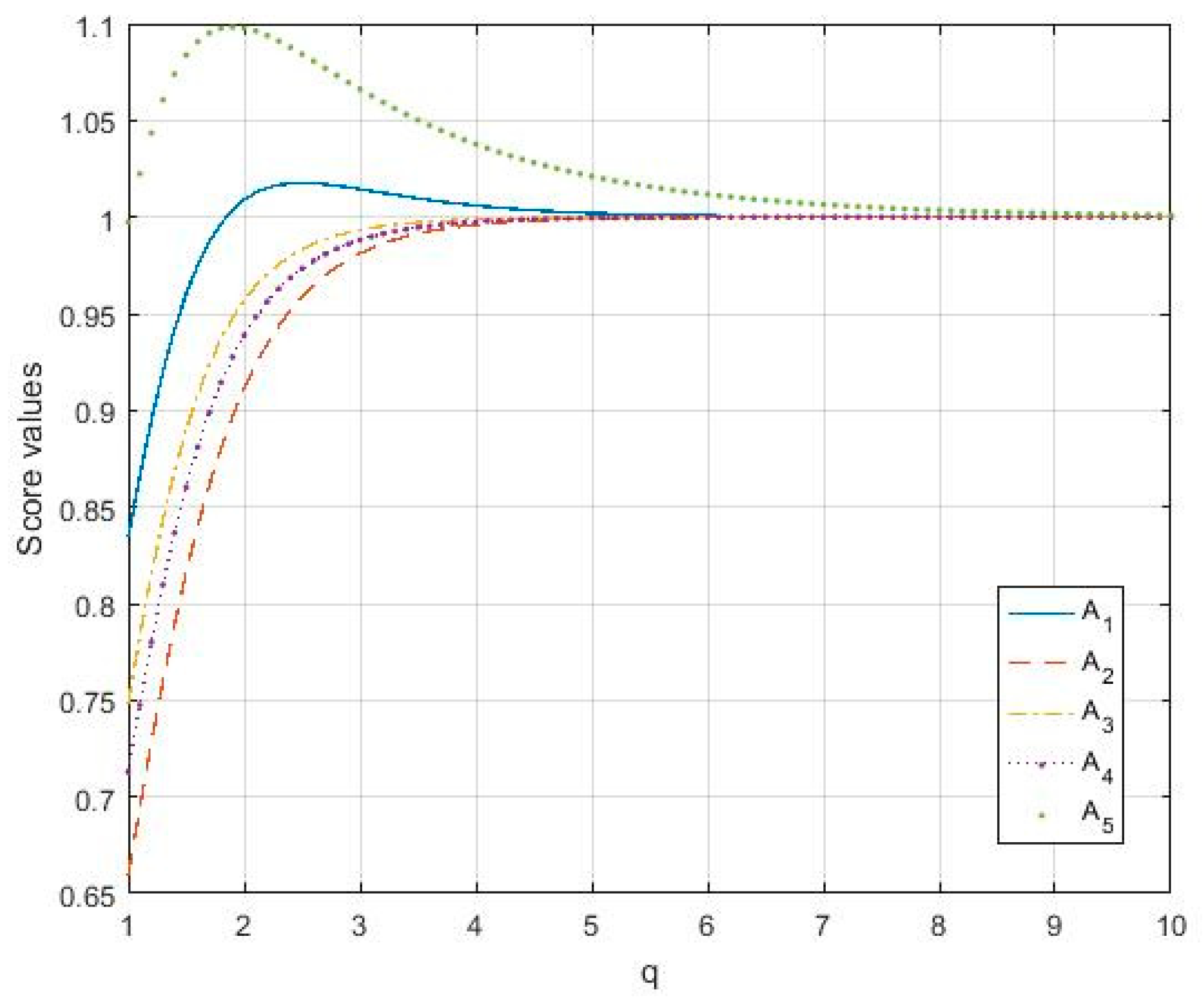
The value of parameter q also has an important influence on the final ranking result of the alternative. In order to analyze the influence of parameter q on the experimental results, we set different q values to solve the above examples, when k = 2 and λ = 2. Figure 1 and Figure 2 show the final ranking results for different q values.

As can be seen from Figure 1, when we use the q-RPFDWHM operator, different values of parameter q will lead to different scores. However, the optimal result is always $A_1$. Furthermore, the scores of all alternatives are decreasing with the increase of the q value and are more and more close to 1. The value of parameter q can reflect the attitudes of decision-makers. The more optimistic the decision-makers are, the smaller the q value is, and the more pessimistic the decision-makers are, the larger the q value is. In real decision scenarios, decision-makers can choose the appropriate q value according to their preferences.

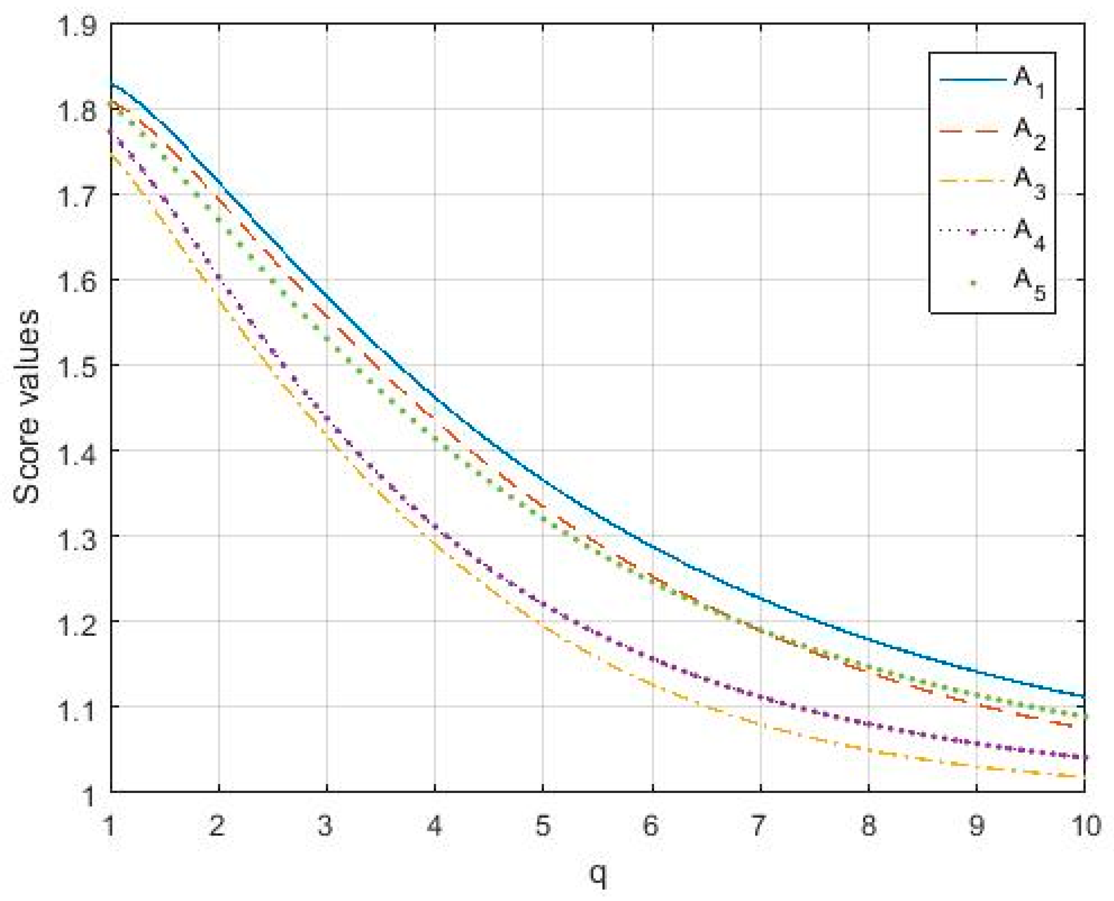
Figure 2 shows that the final score can be different by assigning different q values when utilizing the q-RPFDWDHM operator. However, regardless of the value of q, the final ranking result is the same, that is $A_5>A_1>A_3>A_4>A_2$. Similar to the q-RPFDWHM operator, when the q value is larger, the score value is closer to 1.

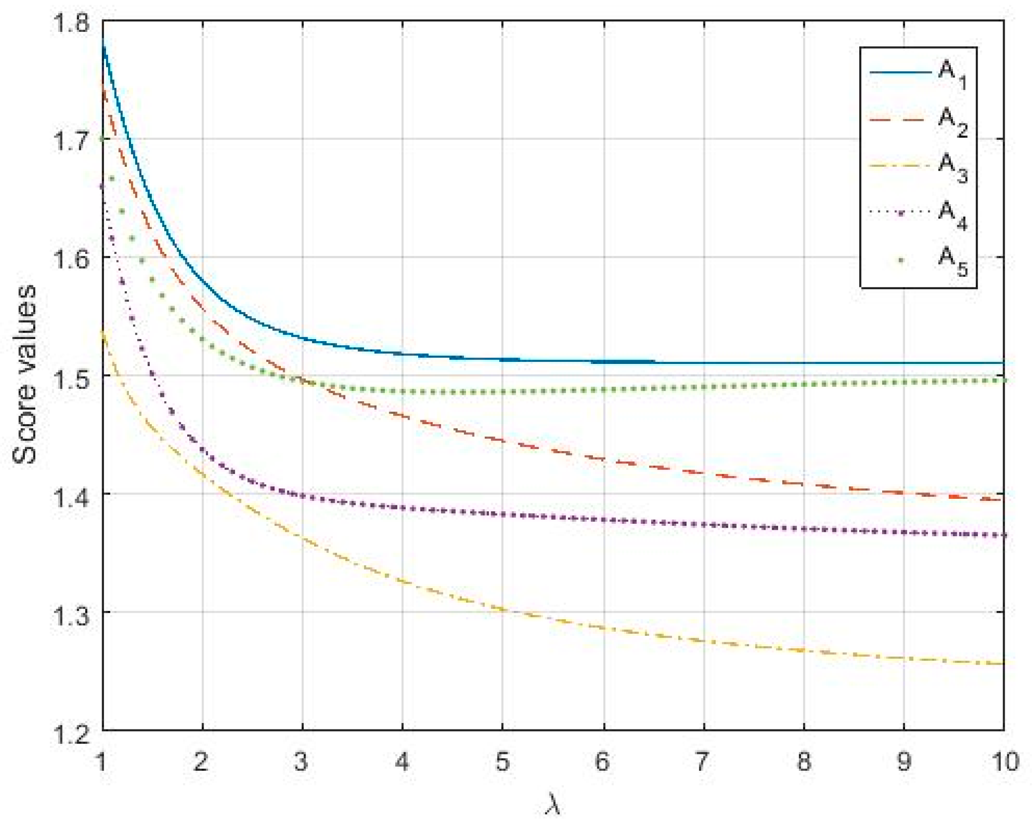
Then, we discuss the impact of the change of λ value on the final score and ranking by setting different λ values in the application of the proposed operator. Let us still use the above example, assuming k = 2, q = 3, and the final results are shown in Figure 3 and Figure 4.

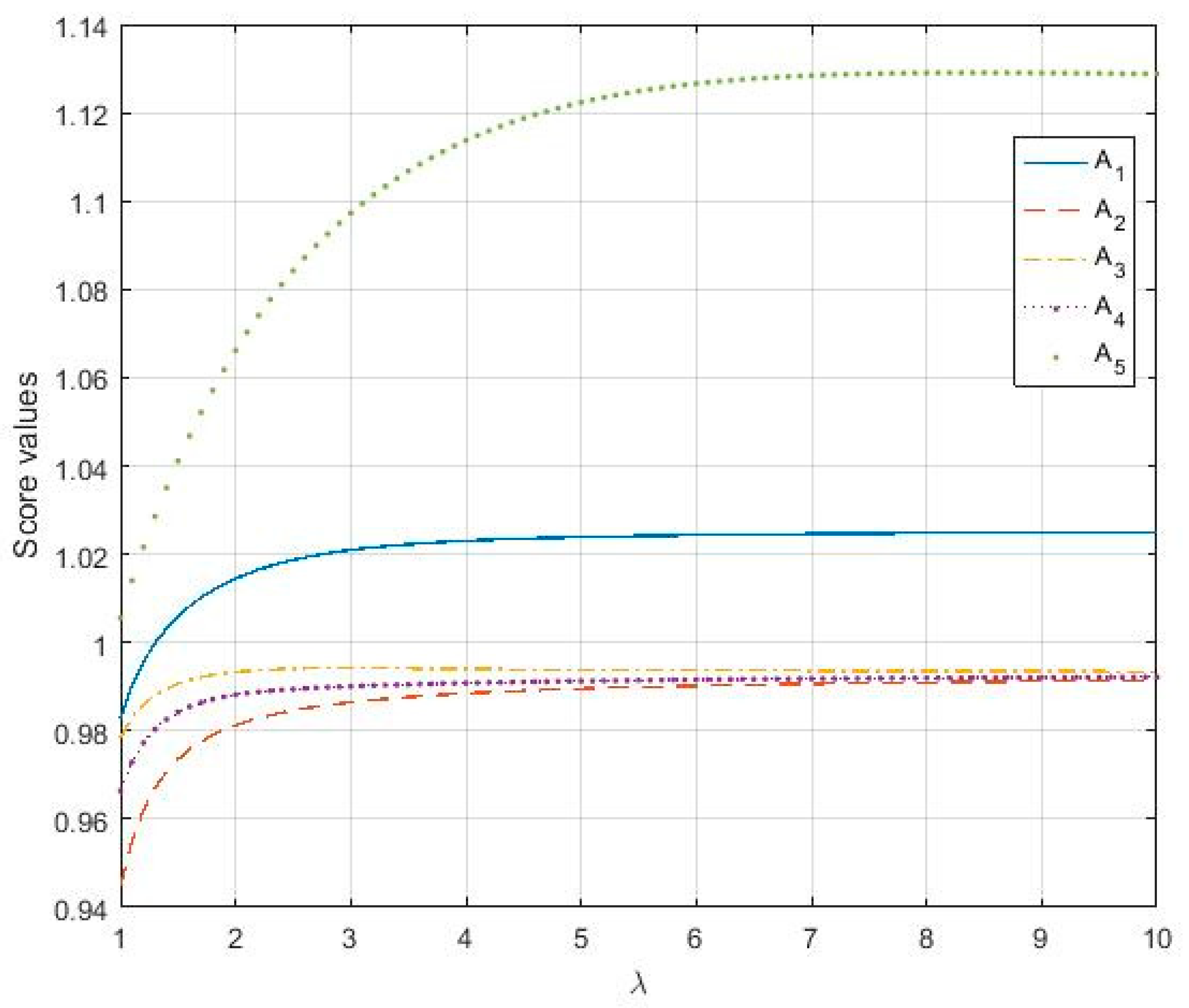
We can draw a conclusion from Figure 3 and Figure 4 that the aggregation results are different with the increase of parameter λ in the proposed operators. However, for the q-RPFDWHM operator, the optimal choice is always $A_1$, and for the q-RPFDWDHM operator, the optimal choice is always $A_5$. Besides, with the increase of λ value, the score value of q-RPFDWHM operator decreases, while the overall evaluation score value of the q-RPFDWDHM operator shows an increasing trend. This shows that the value of λ can reflect the attitude of decision-makers. When using q-RPFDWHM operator, the more optimistic the decision-maker is, the smaller the λ value is, and the more pessimistic the decision-maker is, the larger the λ value is. On the contrary, the more optimistic the decision-maker is, the greater the value of λ, and the more pessimistic the decision-maker is, the smaller the value of λ is when using a q-RPFDWDHM operator. In practical decision-making, the decision-maker can choose the appropriate λ value according to his preference.

5.3. Comparative Analysis

Recently, the application of fuzzy theory to multi-attribute group decision making has become a hot research area. Obviously, q-RPFNs is developed from PFNs and q-ROFNs, which is the basis of our proposed method. Thus, in order to further demonstrate the advantages and superiorities of the proposed operators, we compare the proposed method with some picture fuzzy operators and some q-rung orthopair fuzzy operators, respectively.

5.3.1. Compared with Some Picture Fuzzy Operators

In this section, to better illustrate the validity of the proposed method, we compare our method with that proposed by Wei [13] based on the picture fuzzy weighted average (PFWA) operator, that introduced by Wei [15] based on the picture fuzzy Hamacher weighted average (PFHWA) operator, that presented by Jana et al. [16] based on the picture fuzzy Dombi weighted average (PFDWA) operator, that put forward by Zhang et al. [17] based on the picture fuzzy Dombi weighted Heronian mean (PFDWHM) operator, and that proposed by the Ashraf et al. [41] proposed by the spherical fuzzy weighted average (SFWA) operator. In order to compare these operators, we use each method to solve the above example and present the score values and ranking orders of various methods in

Table 8. Score values and ranking results using our operator and other picture fuzzy operators.

Methods	$\mathit{S}\left({\mathit{\alpha }}_{\mathit{i}}\right),\mathit{i}=1,2,3,4,5$	Ranking Results
Wei’s [13] PFWA operator	$S\left({\alpha }_1\right)=0.490$, $S\left({\alpha }_2\right)=0.367$, $S\left({\alpha }_3\right)=0.365$, $S\left({\alpha }_4\right)=0.440$, $S\left({\alpha }_5\right)=0.525$	$A_5>A_1>A_4>A_2>A_3$
Wei’s [15] PFHWA operator (γ = 2)	$S\left({\alpha }_1\right)=0.739$, $S\left({\alpha }_2\right)=0.669$, $S\left({\alpha }_3\right)=0.668$, $S\left({\alpha }_4\right)=0.710$, $S\left({\alpha }_5\right)=0.758$	$A_5>A_1>A_4>A_2>A_3$
Jana et al.’s [16] PFDWA operator (R = 1)	$S\left({\alpha }_1\right)=0.769$, $S\left({\alpha }_2\right)=0.724$, $S\left({\alpha }_3\right)=0.727$, $S\left({\alpha }_4\right)=0.748$,$S\left({\alpha }_5\right)=0.776$	$A_5>A_1>A_4>A_3>A_2$
Zhang et al.’s [17] PFDWHM operator (λ = 2, p = q = 1)	$S\left({\alpha }_1\right)=0.008$, $S\left({\alpha }_2\right)=-0.088$, $S\left({\alpha }_3\right)=-0.052$, $S\left({\alpha }_4\right)=-0.035$, $S\left({\alpha }_5\right)=0.039$	$A_5>A_1>A_4>A_3>A_2$
Ashraf et al.’s [41] SFWA operator	$S\left({\alpha }_1\right)=0.760$, $S\left({\alpha }_2\right)=0.721$, $S\left({\alpha }_3\right)=0.702$, $S\left({\alpha }_4\right)=0.740$, $S\left({\alpha }_5\right)=0.785$	$A_5>A_1>A_4>A_2>A_3$
the q-RPFDWHM operator in this paper (k = 2, λ = 2, q = 3)	$S\left({\alpha }_1\right)=1.580$, $S\left({\alpha }_2\right)=1.556$, $S\left({\alpha }_3\right)=1.417$, $S\left({\alpha }_4\right)=1.438$,$S\left({\alpha }_5\right)=1.531$	$A_1>A_2>A_5>A_4>A_3$
the q-RPFDWDHM operator in this paper (k = 2, λ = 2, q = 3)	$S\left({\alpha }_1\right)=1.015$, $S\left({\alpha }_2\right)=0.981$, $S\left({\alpha }_3\right)=0.993$, $S\left({\alpha }_4\right)=0.988$, $S\left({\alpha }_5\right)=1.066$	$A_5>A_1>A_3>A_4>A_2$

.

From Table 8, it is obvious that the ranking results obtained by our method based on the q-RPFDWDHM operator are only slightly different from those obtained by other methods, and the best option always is $A_5$. This proves the effectiveness of our method. Compared with PFNs, q-RPFNs can cover more information, so our method can be applied to a wider range of MAGDM environments.

In these methods, Wei’s [13] method based on the PFWA operator and Ashraf et al.’s [41] method based on the SFWA operator both use the simple weighted averaging operator, which leads to their lack of flexibility in aggregating information. Although Ashraf et al.’s [41] SFWA operator based on SFNs is better than Wei’s [13] PFWA operator based on PFNs, it is far inferior to our operators based on q-RPFNs. PFNs and SFNs are special cases of q-RPFNs (q = 1, 2). Furthermore, the simple algebraic operation is a special case of DTT. So, the method we proposed is more general and flexible.

Wei’s [15] method based on the PFHWA operator and Jana et al.’s [16] method based on the PFDWA operator use Hamacher t-norm and t-conorm and DTT, respectively. This makes them more flexible than the PFWA operator proposed by Wei’s [13] and the SFWA operator proposed by Ashraf et al. [41], but all of them ignore the correlation between attributes. Our method applies DTT and Hamy Mean to q-RPFNs, which takes into account the interrelationship among attributes and has strong flexibility and is superior to these methods.

The method based on the PFDWHM operator proposed by Zhang et al. [17] is based on DTT and Heronian Mean. It has high flexibility and takes into account the relationship between attributes. However, it can only capture the relationship between any two parameters. The proposed q-RPFDWHM and q-RPFDWDHM operators based on parameter k can capture the relationship between more than two parameters (at most n − 1 arguments). In addition, our method based on q-RPFNs can contain more information and is more suitable for MAGDM problems.

To sum up, our method based on the q-RPFDWHM operator and the q-RPFDWDHM operator can not only capture the relationship between multiple attributes to imitate a more realistic decision-making environment, but also make the information aggregation process more flexible and effective by using DTT. Compared with other methods, our methods are more flexible and suitable for addressing MAGDM problems.

5.3.2. Compared with Some q-Rung Orthopair Fuzzy Operators

In the section, we compare our proposed method with that proposed by Liu and Wang [25] based on the q-rung orthopair fuzzy weighted average (q-ROFWA) operator, that presented by PD Liu and JL Liu [42] based on the q-rung orthopair fuzzy weighted Bonferroni mean (q-ROFWBM) operator, that put forward by Wei et al. [43] based on the q-rung orthopair fuzzy weighted Heronian mean (q-ROFWHM) operator, and that introduced by Wei et al. [44] based on the q-rung orthopair fuzzy weighted Maclaurin symmetric mean (q-ROFWMSM) operator.

It should be noted that q-ROFNs only have membership degree and non-membership degree, which is a special case of q-RPFNs (the neutral membership degree = 0), so they cannot deal with q-RPFNs. Therefore, in order to compare our proposed method with these methods, we use a new example (adopted from Reference [42]) about the investment for five possible companies $A_i(i=1,2,\dots ,5)$, and set the degree of neutral membership to 0 in our proposed operator. Three decision-makers $D_k(k=1,2,3)$ with weight vector $\lambda ={\left(0.35,0.40,0.25\right)}^T$ are invited to give the evaluation values, and four attributes (let their weight vector be $\varpi ={\left(0.2,0.1,0.3,0.4\right)}^T$) are defined as follows: The risk analysis (C₁), the growth analysis (C₂), the social-political impact analysis (C₃), and the environmental impact analysis (C₄). The decision-makers $D_k(k=1,2,3)$ evaluate the companies $A_i(i=1,2,\dots ,5)$ with respect to the attributes C_j (j = 1, 2, 3, 4) by the q-ROFNs and so the original decision matrix $A^k={\left({\alpha }_{ij}^k\right)}_{5\times 4}$ is shown in

Table 9. The original fuzzy decision matrix A¹ given by D_1.

	C1	C2	C3	C4
$A_1$	$\left(0.5,0.4\right)$	$\left(0.5,0.3\right)$	$\left(0.2,0.6\right)$	$\left(0.4,0.4\right)$
$A_2$	$\left(0.7,0.3\right)$	$\left(0.7,0.3\right)$	$\left(0.6,0.2\right)$	$\left(0.6,0.2\right)$
$A_3$	$\left(0.5,0.4\right)$	$\left(0.6,0.4\right)$	$\left(0.6,0.2\right)$	$\left(0.5,0.3\right)$
$A_4$	$\left(0.8,0.2\right)$	$\left(0.7,0.2\right)$	$\left(0.4,0.2\right)$	$\left(0.5,0.2\right)$
$A_5$	$\left(0.4,0.3\right)$	$\left(0.4,0.2\right)$	$\left(0.4,0.5\right)$	$\left(0.4,0.6\right)$

,

Table 10. The original fuzzy decision matrix A² given by D_2.

	C1	C2	C3	C4
$A_1$	$\left(0.4,0.5\right)$	$\left(0.6,0.2\right)$	$\left(0.5,0.4\right)$	$\left(0.5,0.3\right)$
$A_2$	$\left(0.5,0.4\right)$	$\left(0.6,0.2\right)$	$\left(0.6,0.3\right)$	$\left(0.7,0.3\right)$
$A_3$	$\left(0.4,0.5\right)$	$\left(0.3,0.5\right)$	$\left(0.4,0.4\right)$	$\left(0.2,0.6\right)$
$A_4$	$\left(0.5,0.4\right)$	$\left(0.7,0.2\right)$	$\left(0.4,0.4\right)$	$\left(0.6,0.2\right)$
$A_5$	$\left(0.6,0.3\right)$	$\left(0.7,0.2\right)$	$\left(0.4,0.2\right)$	$\left(0.7,0.2\right)$

and

Table 11. The original fuzzy decision matrix A³ given by D_3.

	C1	C2	C3	C4
$A_1$	$\left(0.4,0.2\right)$	$\left(0.5,0.2\right)$	$\left(0.5,0.3\right)$	$\left(0.5,0.2\right)$
$A_2$	$\left(0.5,0.3\right)$	$\left(0.5,0.3\right)$	$\left(0.6,0.2\right)$	$\left(0.7,0.2\right)$
$A_3$	$\left(0.4,0.4\right)$	$\left(0.3,0.4\right)$	$\left(0.4,0.3\right)$	$\left(0.3,0.3\right)$
$A_4$	$\left(0.5,0.3\right)$	$\left(0.5,0.3\right)$	$\left(0.3,0.5\right)$	$\left(0.5,0.2\right)$
$A_5$	$\left(0.6,0.2\right)$	$\left(0.6,0.4\right)$	$\left(0.4,0.4\right)$	$\left(0.6,0.3\right)$

and presents the score values and ranking orders of various methods in

Table 12. Score values and ranking results using our operator and some q-rung orthopair fuzzy operators.

Methods	$\mathit{S}\left({\mathit{\alpha }}_{\mathit{i}}\right),\mathit{i}=1,2,3,4,5$	Ranking Results
Liu and Wang’s [25] q-ROFWA operator (q = 3)	$S\left({\alpha }_1\right)=0.062$$,S\left({\alpha }_2\right)=0.236$$,S\left({\alpha }_3\right)=0.034$$,S\left({\alpha }_4\right)=0.157$$,S\left({\alpha }_5\right)=0.138$	$A_2>A_4>A_5>A_1>A_3$
Liu, P.D. and Liu, J.L.’s [42] q-ROFWBM operator (q = 3, s = t = 1)	$S\left({\alpha }_1\right)=-0.771$, $S\left({\alpha }_2\right)=-0.712$, $S\left({\alpha }_3\right)=-0.794$, $S\left({\alpha }_4\right)=-0.729$, $S\left({\alpha }_5\right)=-0.761$	$A_2>A_4>A_5>A_1>A_3$
Wei et al.’s [43] q-ROFWHM operator (q = 3, ϕ = ϕ = 1)	$S\left({\alpha }_1\right)=0.436$, $S\left({\alpha }_2\right)=0.523$, $S\left({\alpha }_3\right)=0.419$, $S\left({\alpha }_4\right)=0.493$, $S\left({\alpha }_5\right)=0.471$	$A_2>A_4>A_5>A_1>A_3$
Wei et al.’s [44] q-ROFWMSM operator (k = 2, q = 3)	$S\left({\alpha }_1\right)=0.910$, $S\left({\alpha }_2\right)=0.944$, $S\left({\alpha }_3\right)=0.900$, $S\left({\alpha }_4\right)=0.926$, $S\left({\alpha }_5\right)=0.924$	$A_2>A_4>A_5>A_1>A_3$
the q-RPFDWHM operator in this paper (k = 2, λ = 2, q = 3)	$S\left({\alpha }_1\right)=1.296$, $S\left({\alpha }_2\right)=1.552$, $S\left({\alpha }_3\right)=1.293$, $S\left({\alpha }_4\right)=1.526$, $S\left({\alpha }_5\right)=1.445$	$A_2>A_4>A_5>A_1>A_3$
the q-RPFDWDHM operator in this paper (k = 2, λ = 2, q = 3)	$S\left({\alpha }_1\right)=0.854$, $S\left({\alpha }_2\right)=0.986$, $S\left({\alpha }_3\right)=0.766$, $S\left({\alpha }_4\right)=0.933$, $S\left({\alpha }_5\right)=0.838$	$A_2>A_4>A_1>A_5>A_3$

.

As shown in Table 12, it is obvious to find that the final ranking results using other methods are almost the same as those of our proposed methods and the best option always is $A_2$. It shows that our method is very effective. Compared with q-RPFNs, q-ROFNs do not have the degree of neutral membership, which will lead to the loss of some information. Our method is based on DTT, which can aggregate relevant information more comprehensively, provide decision-makers with more a flexible choice environment, and make decisions more accurate and powerful.

Liu and Wang’s [25] method is based on the q-ROFWA operator, which assumes that the attributes are relatively independent, and does not take into account the correlation between the attributes. The proposed method based on q-RPFDWHM operator and q-RPFDWDHM operator can well reflect the correlation among attributes and use DTT operation rules to show the attitude of decision-makers.

Liu, P.D., and Liu, J.L.’s [42] and Wei et al.’s [43] method based on the Bonferroni mean and Heronian mean operators respectively. The advantage of these two operators over the method proposed by Liu and Wang [25] is that they take account of the correlation between attributes, but they can only capture the correlation between any two attributes, and our method can capture the correlation between multiple attributes (at most n − 1 arguments) by setting the parameter k. That’s to say, our method is more practical and more suitable for MAGDM problems.

Wei et al.’s [44] method is based on the Maclaurin symmetric mean operator, which is a special case of HM and can also capture the correlation between any two attributes. It is worth mentioning that our method is based on the q-RPFDWHM operator and the q-RPFDWDHM operator, which also have a parameter λ which can reflect the attitudes of decision-makers. The different values of parameter λ represent different decision-making attitudes. Decision-makers can adjust the values of parameters according to their own interests and actual needs, so as to obtain more appropriate solutions.

Through the above analysis, the advantages of our method based on the q-RPFDWHM operator and the q-RPFDWDHM operator are obvious, which can be summarized as follows: First, our method is based on q-RPFNs, which includes non-membership, neutrality, and membership, and gives decision-makers a more flexible environment to avoid information loss in the decision-making process. Secondly, the attributes in real instances are often related. Our method based on the q-RPFDWHM operator and the q-RPFDWDHM operator can capture the correlation between the attributes and simulate the real MAGDM process more effectively. Thirdly, the proposed method based on the q-RPFDWHM operator and the q-RPFDWDHM operator has three different parameters. Decision-makers can set different parameters according to their risk aversion, their own interests, and actual situation, so as to obtain the most appropriate decision-making objectives reasonably, which creates a flexible decision-making environment for decision-makers. Furthermore, the proposed operators provide a new method to aggregate q-RPFNs based on the DTT, which is more general and powerful. Our method is more effective, flexible and powerful, and more suitable for solving MAGDM problems.

6. Conclusions

At present, q-RPFNs have become more popular for dealing with multi-attribute group decision-making problems, because they cannot only contain more information, but also take into account the neutrality of decision-makers. In this paper, we propose novel operational rules of q-rung picture fuzzy numbers (q-RPFNs) on the basis of Dombi t-norm and t-conorm. Then, we apply the traditional Hamy mean operator to q-RPFNs based on the DTT and propose q-RPFDHM, q-RPFDWHM, q-RPFDDHM, and q-RPFDWDHM operators. On this basis, a new solution to the MAGDM problem is proposed and applied to optimal project evaluation. In order to better verify the effectiveness and superiority of this method, we carried out parameter analysis, and compared this method with some picture fuzzy operators and some q-rung orthopair fuzzy operators, respectively. Through analysis, the main advantages of this method are as follows: (1) The use of q-RPFNs can capture more comprehensive information and effectively avoid information loss in the decision-making process. (2) It can capture the correlation among the attributes, which is more suitable for the real decision-making environment. (3) Different parameters can be set to meet various needs, with greater flexibility and versatility. (4) The proposed operators provide a new method to aggregate q-RPFNs based on the DTT, which is more general and powerful.

In future work, we will apply our method to more practical and more extensive MAGDM problems. Considering the validity and extensiveness of the Hamy mean operator and DTT operation paradigm, we will study them in a more ambiguous environment, such as in hesitant decision-making.