Unified Local Convergence for Newton’s Method and Uniqueness of the Solution of Equations under Generalized Conditions in a Banach Space

Abstract

Under the hypotheses that a function and its Fréchet derivative satisfy some generalized Newton–Mysovskii conditions, precise estimates on the radii of the convergence balls of Newton’s method, and of the uniqueness ball for the solution of the equations, are given for Banach space-valued operators. Some of the existing results are improved with the advantages of larger convergence region, tighter error estimates on the distances involved, and at-least-as-precise information on the location of the solution. These advantages are obtained using the same functions and Lipschitz constants as in earlier studies. Numerical examples are used to test the theoretical results.

1. Introduction

Let $\mathbb{X}$ and $\mathbb{Y}$ be Banach spaces. Let $U(x,r)$ and $\overline{U}(x,r)$ stand, respectively, for the open and closed ball in $\mathbb{X}$ with center x and radius $r>0$. Denote by $\mathsf{Ł}(\mathbb{X},\mathbb{Y})$ the space of bounded linear operators from $\mathbb{X}$ into $\mathbb{Y}$. Further, let $D\subset X$ be a nonempty set.

In the present paper, we are concerned with the problem of approximating a locally unique solution $x^{*}$ of the equation

$$F(x)=0,$$

(1)

where F is a Fréchet continuously differentiable operator, defined on D with values in $\mathbb{Y}$.

Numerous applications from applied mathematics, optimization, mathematical biology, chemistry, economics, physics, engineering, and other disciplines can be brought, in the form of Equation (1) by mathematical modelling [1,2,3,4,5,6,7,8,9]. The solution of these equations can rarely be found in closed form. Hence, the solution methods for these equations are iterative. In particular, the practice of numerical analysis for finding such solutions is essentially connected to variants of iterative methods [1,2,3,4,5,6,7,8,9,10,11,12,13,14,15,16,17,18,19,20,21,22,23]. Research about the convergence issues of Newton methods involves two types: Semi-local and local convergence analysis. The semi-local convergence issue is, based on the information around an initial point, to give criteria ensuring the convergence of iterative methods; meanwhile, the local one is, based on the information around a solution, to find estimates for the radii of the convergence balls. We find, in the literature, several studies on the weakness and/or extension of the hypotheses made on the underlying operators. There is a plethora on local, as well as semi-local, convergence results; we refer the reader to [1,2,3,4,5,6,7,8,9,10,11,12,13,14,15,16,17,18,19,20,21,22,23]. In this paper, we assume the existence of $x^{*}$, but do not address any existence results.

Newton’s method is defined by the iterative procedure

$$\begin{array}{c}{x}_0\mathrm{is}\mathrm{an}\mathrm{initial}\mathrm{point}\hfill \\ x_{n+1}=x_n-F^{\prime }{(x_n)}^{-1}F(x_n)\mathit{for}\mathrm{each}n=0,1,2,\cdots ,\hfill \end{array}$$

(2)

and is, undoubtedly, one of the most popular iterative processes for generating a sequence $\left\{x_n\right\}$ approximating $x^{*}$. Here, $F^{\prime }(x)\in \mathsf{Ł}(\mathbb{X},\mathbb{Y})$ denotes the Fréchet derivative of F at $x\in \overline{U}(x_0,R)$.

Newton–Mysovskii-type conditions (see (10) ) have been used by several authors [4,7,9,12,21,22] to provide a local, as well as a semi-local, convergence for Newton’s method and Newton-like methods.

A very important problem in the study of iterative procedures is the convergence region. Some of the existing results provide conditions for the convergence, based on small regions under certain conditions. Therefore, it is important to enlarge the convergence region without additional hypotheses. Another important problem is to find more precise error estimates on the distance $\parallel x_n-x^{*}\parallel$, as well as uniqueness of the solution results. These are our objectives in this paper.

In particular, we obtain the following advantages over earlier works:

(a₁)

At least as large a radius of convergence to at least as many choices of initial points;

(a₂)

At least as small a ratio of convergence, so at most as few iterates must be computed to obtain a desired error tolerance; and

(a₃)

The information on the location of the solution is at least as precise.

It is worth noticing that these advantages are obtained, although more general and flexible majorant-type conditions are used.

Indeed these advantages are obtained by specializing the new majorant functions. Hence, the applicability of Newton’s method is extended. Our approach can be used to improve local and semi-local results for Newton-like methods, secant-type methods, and other single- or multi-step methods along the same lines.

The paper is structured as follows: Section 2 contains the local convergence analysis of Newton’s method. Applications are given in the Section 3. Our findings are summarized in Section 4.

2. Local Convergence Analysis

We present the main local convergence result for Newton’s method.

Theorem 1.

Let $F:D\subset X\to Y$ be a Fréchet-differentiable operator. Suppose:

(a)

There exists $x^{*}\in D$ such that $F(x^{*})=0$ and $F^{\prime }{(x)}^{-1}\in \mathsf{Ł}(\mathbb{Y},\mathbb{X})$ for all $x\in D$.

(b)

There exists a function $\phi :[0,+\infty )\to [0,+\infty )$ with $\phi (0)=0$ such that $\frac{\phi (t)}{t^{1+\lambda }}$ is continuous, where $t\ne 0$, and is non-decreasing for some $\lambda \ge 0$.

(c)

For all $x\in D$

$$\parallel F^{\prime }{(x)}^{-1}(F(x)-F^{\prime }(x)(x-x^{*}))\parallel \le \phi (\parallel x-x^{*}\parallel )\parallel x-x^{*}\parallel .$$

(d)

There exists a minimal root $\varrho >0$ of equation $\phi (t)=1$, such that

$${\displaystyle \frac{\phi (\varrho )}{{\varrho }^{\lambda }}}\le 1.$$

(e)

$\overline{U}(x^{*},\varrho )\subseteq D.$

Then, the sequence $\left\{x_n\right\}$ generated for $x_0\in \mathrm{U}(x^{*},\varrho )-\left\{x^{*}\right\}$ by Newton’s method is well-defined, stays in U$(x^{*},\varrho )$ for all $n=0,1,2,\dots$, and converges to $x^{*}$; which is the only root of the equation $F(x)=0$ in $U(x^{*},\varrho )$. Moreover, the following estimate holds

$$\begin{array}{c}\hfill \parallel x_n-x^{*}\parallel \le e_n,n=0,1,2,\dots \end{array}$$

(3)

where

$$\begin{array}{c}\hfill q={\displaystyle \frac{\phi (\parallel x_0-x^{*}\parallel )}{\parallel x_0-x^{*}{\parallel }^{\lambda }}}\in [0,1),\end{array}$$

(4)

and $e_n={\displaystyle \frac{{\left(q^{\frac{1}{\lambda }}\parallel x_0-x^{*}\parallel \right)}^{{(1+\lambda )}^n}}{q^{\frac{1}{\lambda }}}}$.

Proof. 

By $(b)$ and $(d)$, and using (4), we have that

$$\begin{array}{ccc}q\hfill & =& {\displaystyle \frac{\phi (\parallel x_0-x^{*}\parallel )\parallel x_0-x^{*}\parallel }{\parallel x_0-x^{*}{\parallel }^{1+\lambda }}}\le {\displaystyle \frac{\phi (\varrho )}{{\varrho }^{1+\lambda }}}\parallel x_0-x^{*}\parallel \hfill \\ & \le & {\displaystyle \frac{\parallel x_0-x^{*}\parallel }{\varrho }}<1.\hfill \end{array}$$

(5)

If $x_k\in U(x^{*},\varrho )$, then, by Newton’s method, we can write

$$\begin{array}{ccc}{x}_{k+1}-x^{*}\hfill & =& x_k-x^{*}-F^{\prime }{(x_k)}^{-1}F(x_k)\hfill \\ & =& -F^{\prime }{(x_k)}^{-1}(F(x_k)-F^{\prime }(x_k)(x_k-x^{*})),\hfill \end{array}$$

(6)

and so, by $(c)$ and (6),

$$\parallel x_{k+1}-x^{*}\parallel \le \phi (\parallel x_k-x^{*}\parallel )\parallel x_k-x^{*}\parallel .$$

(7)

If $k=0$ in (7), we obtain, by (4) and (5), that

$$\parallel x_1-x^{*}\parallel \le \phi (\parallel x_0-x^{*}\parallel )\parallel x_0-x^{*}\parallel <\parallel x_0-x^{*}\parallel <\varrho .$$

Hence, $x_1\in U(x^{*},\varrho )$; that is, (7) can be obtained for $k=0,1,\dots$. By mathematical induction, all $x_k\in U(x^{*},\varrho )$ and $\parallel x_k-x^{*}\parallel$ decreases monotonically. Moreover, for all $k=0,1,\dots$, we consequently obtain, from $(b)$ and (7), that

$$\begin{array}{ccc}\parallel x_{k+1}-x^{*}\parallel \hfill & \le & {\displaystyle \frac{\phi (\parallel x_k-x^{*}\parallel )}{\parallel x_k-x^{*}{\parallel }^{1+\lambda }}}\parallel x_k-x^{*}{\parallel }^{1+\lambda }\parallel x_k-x^{*}\parallel \hfill \\ & \le & {\displaystyle \frac{\phi (\parallel x_0-x^{*}\parallel )}{\parallel x_0-x^{*}{\parallel }^{1+\lambda }}}\parallel x_k-x^{*}{\parallel }^{1+\lambda }\parallel x_k-x^{*}\parallel \hfill \\ & \le & {\displaystyle \frac{\phi (\parallel x_0-x^{*}\parallel )}{\parallel x_0-x^{*}{\parallel }^{1+\lambda }}}\parallel x_0-x^{*}\parallel \parallel x_k-x^{*}{\parallel }^{\lambda +1}\hfill \\ & =& {\displaystyle \frac{\phi (\parallel x_0-x^{*}\parallel )}{\parallel x_0-x^{*}{\parallel }^{\lambda }}}{\parallel x_k-x^{*}\parallel }^{\lambda +1}\hfill \\ & =& q\parallel x_k-x^{*}{\parallel }^{\lambda +1}\hfill \\ & \le & q(q\parallel x_{k-1}-x^{*}{{\parallel }^{\lambda +1})}^{\lambda +1}\hfill \\ & =& q^{1+(\lambda +1)}q\parallel x_{k-1}-x^{*}{\parallel }^{{(\lambda +1)}^2})\hfill \\ & \le & \dots \hfill \\ & \le & e_{k+1},\hfill \end{array}$$

(8)

which implies (3). Notice that, as $q^{\frac{1}{\lambda }}\parallel x_0-x^{*}\parallel <1$, we have ${\displaystyle \underset{n\to \infty }{lim}{e}_n=0}$ and so ${\displaystyle \underset{n\to \infty }{lim}{x}_n=x^{*}}$. Let $y^{*}\in U(x^{*},\varrho )$ with $F(y^{*})=0$. Replace $x^{*}$ by $y^{*}$ in (6)–(8). Then, we have that

$$\parallel x_{k+1}-y^{*}\parallel \le q\parallel x_k-y^{*}{\parallel }^{\lambda +1},$$

(9)

and so ${\displaystyle \underset{k\to \infty }{lim}{x}_k=y^{*}}$. However, we showed that ${\displaystyle \underset{k\to \infty }{lim}{x}_k=x^{*}}$. Hence, we conclude that $x^{*}=y^{*}$. □

Remark 1.

Estimate $(c)$ generalizes the Newton–Mysovskii-type conditions, already in the literature [4,7,9,12,21,22], of the form

$$\parallel F^{\prime }{(z)}^{-1}(F(x)-F(y)-F^{\prime }(x)(x-y)){\parallel \le K\parallel x-y\parallel }^{\mu },K>0,\mu \in [0,2],$$

(10)

for each $x,y,z\in D$, if we choose $\overline{\phi (t)}=K{t}^{\mu -1}$. However, in this paper, we use the weaker condition

$$\parallel F^{\prime }{(x)}^{-1}(F(x)-F(x^{*})-F^{\prime }(x)(x-x^{*}))\parallel \le K_0{\parallel x-x^{*}\parallel }^{\mu },K_0>0.$$

Thus, the function φ specializes to ${\phi }_0(t)=K_0{t}^{\mu -1}$ for $z=x$ and $y=x^{*}$. Then, we have ${\phi }_0(t)\le \overline{\phi (t)}$, so $K_0\le K$. Moreover, (10) implies $(c)$ in this case, but not necessarily vice versa. Hence, the new results, in this case, are better than the old ones. It is worth noticing that these improvements are obtained under weaker conditions (see also the numerical examples), since, as $K_0\le K$, the new radii are larger and the new ratio is smaller.

In the case where $(c)$ is difficult to verify, we have the following alternative.

Theorem 2.

Let $F:D\subset X\to Y$ be a Fréchet-differentiable operator. Suppose:

(a)

There exists an $x^{*}\in D$ and a function $w_0:{\mathbb{R}}_{+}\to {\mathbb{R}}_{+}$ which is continuous and nondecreasing, with $w_0(0)=0$, such that

$$F(x^{*})=0,F^{\prime }{(x^{*})}^{-1}\in \mathsf{Ł}(\mathbb{Y},\mathbb{X}),$$

and, for all $x\in D$,

$$\parallel F^{\prime }{(x^{*})}^{-1}(F^{\prime }(x)-F^{\prime }(x^{*}))\parallel \le w_0(\parallel x-x^{*}\parallel ).$$

The equation

$$w_0(t)=1$$

has a minimal positive root, denoted by $r_0$. Set $D_0=D\cap U(x^{*},r_0)$.

(b)

There exists a function $w:{\mathbb{R}}_{+}\to {\mathbb{R}}_{+}$ which is continuous and non-decreasing with $w(0)=0$ such that, for all $x\in D_0$,

$$\parallel F^{\prime }{(x^{*})}^{-1}(F(x)-F^{\prime }(x)(x-x^{*}))\parallel \le w(\parallel x-x^{*}\parallel )\parallel x-x^{*}\parallel .$$

(c)

The equation

$$w(t)+(w_0(t)-1)t^{\lambda }=0,\mathit{for}\mathit{some}\lambda \ge 0,$$

has a smallest root, $r^{*}\in [0,r_0)$.

(d)

The function $\frac{w(t)}{t^{\lambda }(1-w_0(t))}$ is continuous and nondecreasing on the interval $(0,r_0)$.

(e)

$\overline{U}(x^{*},r^{*})\subseteq D$.

Then, the sequence $\left\{x_n\right\}$ generated for $x_0\in \mathrm{U}(x^{*},r^{*})-\left\{x^{*}\right\}$ by Newton’s method is well-defined, remains in U$(x^{*},r^{*})$ for all $n=0,1,2,\dots$, and converges to $x^{*}$, which is the only root of the equation $F(x)=0$ in $D_2=U(x^{*},r^{*})\cap D$. Moreover, the following estimates hold

$$\begin{array}{ccc}\parallel x_{n+1}-x^{*}\parallel \hfill & \le & {\displaystyle \frac{w(\parallel x_n-x^{*}\parallel )\parallel x_n-x^{*}\parallel }{1-w_0(\parallel x_n-x^{*}\parallel )}}\hfill \\ & \le & {\displaystyle \frac{w(\parallel x_n-x^{*}\parallel )\parallel x_n-x^{*}{\parallel }^{\lambda +1}}{\parallel x_n-x^{*}{\parallel }^{\lambda }(1-w_0(\parallel x_n-x^{*}\parallel ))}}\hfill \\ & \le & q_0\parallel x_n-x^{*}{\parallel }^{1+\lambda }\le \parallel x_n-x^{*}\parallel <r^{*},\hfill \end{array}$$

(11)

where

$$\begin{array}{c}\hfill q_0={\displaystyle \frac{w(\parallel x_0-x^{*}\parallel )}{\parallel x_0-x^{*}{\parallel }^{\lambda }(1-w_0(\parallel x_0-x^{*}\parallel ))}}\in [0,1).\end{array}$$

(12)

Proof. 

We have that, for all $x\in \overline{U}(x^{*},r^{*})$,

$$\parallel F^{\prime }{(x^{*})}^{-1}(F^{\prime }(x)-F^{\prime }(x^{*}))\parallel \le w_0(\parallel x-x^{*}\parallel )\le w_0(r^{*})<1$$

(13)

by $(a)$, $(c)$, and the definition of $r^{*}$. It follows, from (13) and the Banach Lemma on invertible operators [7,22], that $F^{\prime }{(x)}^{-1}\in \mathsf{Ł}(\mathbb{Y},\mathbb{X})$ and

$$\parallel F^{\prime }{(x)}^{-1}{F}^{\prime }(x^{*})\parallel \le {\displaystyle \frac{1}{1-w_0(\parallel x-x^{*}\parallel )}}.$$

(14)

Define the function φ on the interval $[0,r^{*})$ by

$$\phi (t)={\displaystyle \frac{w(t)}{1-w_0(t)}}.$$

(15)

Then, the result follows from the proof of Theorem 1, by noticing that

$$\begin{array}{ccc}\parallel x_{k+1}-x^{*}\parallel \hfill & =& \parallel \left[F^{\prime }{(x_k)}^{-1}{F}^{\prime }(x^{*})\right]\left[F^{\prime }{(x^{*})}^{-1}(F(x_k)-F^{\prime }(x_k)(x_k-x^{*}))\right]\parallel \hfill \\ & \le & \parallel F^{\prime }{(x_k)}^{-1}{F}^{\prime }(x^{*})\parallel \parallel F^{\prime }{(x^{*})}^{-1}(F(x_k)-F^{\prime }(x_k)(x_k-x^{*}))\parallel \hfill \\ & \le & {\displaystyle \frac{w(\parallel x_k-x^{*}\parallel )\parallel x_k-x^{*}\parallel )}{1-w_0(\parallel x_k-x^{*}\parallel )}}=\phi (\parallel x_k-x^{*}\parallel )\parallel x_k-x^{*}\parallel ).\hfill \\ \hfill \square \end{array}$$

The uniqueness of the solution $x^{*}$ depends on the functions $w_0$ and w.

Next, we present a uniqueness result, using only the function $w_0$.

Proposition 3.

Suppose that D is a convex set. Moreover, we assume that

$${\int }_0^1{w}_0(\theta r)d\theta <1,r\ge 0$$

(16)

and

$$\parallel F^{\prime }{(x^{*})}^{-1}(F^{\prime }(x)-F^{\prime }(x^{*}))\parallel \le w_0(\parallel x-x^{*}\parallel ),$$

for all $x\in D_3=D\cap U(x^{*},r_0)$, where $w_0:[0,\infty )\to [0,\infty )$ is a continuous and non-decreasing function. Then, the point $x^{*}$ is the only solution of the equation $F(x)=0$ in $D_3$.

Proof. 

The convergence of Newton’s method to the root $x^{*}$ has been established in Theorem 2. Let $y^{*}\in D_3$ with $F(y^{*})=0$. Define $Q={\int }_0^1(F^{\prime }(x^{*}+\theta (y^{*}-x^{*}))d\theta .$ Using (16), we have

$$\parallel F^{\prime }{(x^{*})}^{-1}(Q-F^{\prime }(x^{*}))\parallel \le {\int }_0^1{w}_0(\parallel \theta (x^{*}-y^{*})\parallel )d\theta \le {\int }_0^1{w}_0(\theta r_1)d\theta <1.$$

(17)

Hence, by (17), $Q^{-1}\in \mathsf{Ł}(\mathbb{Y},\mathbb{X})$. Then, from the identity

$$0=F(y^{*})-F(x^{*})=Q(y^{*}-x^{*}),$$

we conclude that $x^{*}=y^{*}$.□

Remark 2.

(a)

If $r=r^{*}$, then, by Theorem 2, we conclude that the root $x^{*}$ is unique in $D_3$.

(b)

The local results obtained in this study are better than the earlier results in [5,9,17,23,24,25,26], even if specialized.

(c)

Case of the Radius Lipschitz condition [9,26]:

$$\parallel F^{\prime }{(x^{*})}^{-1}(F^{\prime }(x)-F^{\prime }(x^{\theta }))\parallel \le {\int }_{\theta \parallel x-x^{*}\parallel }^{\parallel x-x^{*}\parallel }{L}_1(u)du,\mathit{for}\mathit{all}x\in D,$$

(18)

where $L_1$ is a positive integrable function and $x^{\theta }=x^{*}+\theta (x-x^{*})$.

Moreover, in light of (18), there exists a positive integrable function, $L_0$, such that

$$\parallel F^{\prime }{(x^{*})}^{-1}(F^{\prime }(x)-F^{\prime }(x^{*}))\parallel \le {\int }_0^{\parallel x-x^{*}\parallel }{L}_0(u)du,\mathit{for}\mathit{all}x\in D.$$

(19)

Notice that

$$L_0(t)\le L_1(t),\mathit{for}\mathit{all}t\in [0,r_0],$$

(20)

and ${\varrho }_0$ is the minimal positive root of the equation

$${\int }_0^t{L}_0(u)du=1.$$

(21)

The radius of convergence, $r_1$, is obtained in [26] under (18), and is given as the root of the equation

$${\displaystyle \frac{{\int }_0^r{L}_1(u)udu}{r(1-{\int }_0^r{L}_1(u)du)}}=1.$$

(22)

The radius of convergence $\overline{r^{*}}$ found by us, if $D_0=D$ is the positive root of the equation, is

$${\displaystyle \frac{{\int }_0^r{L}_1(u)udu}{r(1-{\int }_0^r{L}_0(u)du)}}=1.$$

(23)

In view of (21)–(23), we have that

$$r_1\le \overline{r^{*}}$$

(24)

Indeed, let the functions $g_0$ and $g_1$ be defined as

$$g_0(r)={\int }_0^r{L}_1(u)udu+r{\int }_0^r{L}_0(u)du-r$$

and

$$g_1(r)={\int }_0^r{L}_1(u)udu+r{\int }_0^r{L}_1(u)du-r.$$

Then, in light of (21), we get

$$g_0(r)\le g_1(r),$$

and, for $r=r_1$,

$$g_0(r)\le g_1(r)=0,$$

by the definition of $r_1$ leading to (24).

We can do even better, if $D_0\ne D$. In this case, the function w (i.e., $L_1$) depends on $w_0$ (i.e., $L_0$), and we have that

$$\parallel F^{\prime }{(x^{*})}^{-1}(F^{\prime }(x)-F^{\prime }(x^{\theta }))\parallel \le {\int }_{\theta \parallel x-x^{*}\parallel }^{\parallel x-x^{*}\parallel }L(u)du,\mathit{for}\mathit{all}x\in D_0\mathit{and}\mathit{all}\theta \in [0,1],$$

(25)

where L is a positive integrable function.

Then, we have that

$$L(u)\le L_1(u)\mathit{for}\mathit{all}u\in [0,{\varrho }_0],$$

(26)

since $D_0\subseteq D$. In general, we do not know which of the functions $L_0$ or L is smaller than the other (see, however, the numerical examples). Then, the radius of convergence $r^{*}$ is the positive solution of the equation

$${\displaystyle \frac{{\int }_0^{r}L(u)udu}{r(1-{\int }_0^r{L}_0(u)du)}}=1,$$

(27)

and we have, by (26), that

$$\overline{r^{*}}\le r^{*},$$

(28)

using a similar proof as the one below (24). Hence, we have that

$$r_1\le \overline{r^{*}}\le r^{*}.$$

(29)

Inequality (29) can be strict, if (22) and (26) are strict inequalities. The corresponding ratios of convergence are also improved (see the numerical examples).

Clearly, (18) (or (26) with $r_0$ replaced by ${\varrho }_0$ in $D_0$) is a special case of condition $(b)$ in Theorem 2 and a special case of condition $(a)$ in Theorem 2.

(d)

Case of Majorant conditions [5,17]:

$$\parallel F^{\prime }{(x^{*})}^{-1}(F^{\prime }(x)-F^{\prime }(x^{\theta }))\parallel \le f_1^{\prime }(\parallel x-x^{*}\parallel )-f_1^{\prime }(\theta \parallel x-x^{*}\parallel ),$$

(30)

where $f_1$ is a convex, strictly increasing function, with $f_1(0)=0$ and $f_1^{\prime }(0)=-1$.

Notice that the following functions are convex, strictly increasing functions with $f_1(0)=0$, and $f_1^{\prime }(0)=-1$:

• $f_1:\mathbb{R}\to \mathbb{R}$ with $f_1(t)=e^t-2t-1$;
• $f_1:[0,1)\to \mathbb{R}$ with $f_1(t)=-ln(1-t)-2$; and
• $f_1:[0,{\displaystyle \frac{1}{a}})\to \mathbb{R}$ with $f_1(t)={\displaystyle \frac{t}{1-at}}-2t,a\ne 0$.

In view of (30), there exists a function $f_0$ with the same properties as $f_1$, such that

$$\parallel F^{\prime }{(x^{*})}^{-1}(F^{\prime }(x)-F^{\prime }(x^{*}))\parallel \le f_0^{\prime }(0)-f_0^{\prime }(\theta \parallel x-x^{*}\parallel ),\mathit{for}\mathit{all}x\in D.$$

(31)

Thus, we can choose

$$w_0(t)=f_0^{\prime }(t)-f_0^{\prime }(0).$$

(32)

By comparing (30) and (31), we get

$$f_0^{\prime }(t)\le f_1^{\prime }(t),\mathit{for}\mathit{all}t\in [0,{\overline{\varrho }}_0].$$

(33)

The radius of convergence $\overline{r_1}$ in [5,17], under (30), is given as the positive root of the equation

$${\displaystyle \frac{f_1(t)-t{f}_1^{\prime }(t)}{t{f}_1^{\prime }(t)}}=1.$$

(34)

In our case, we have that $\overline{r^{*}}$ solves the equation

$${\displaystyle \frac{f_1(t)-t{f}_1^{\prime }(t)}{t{f}_0^{\prime }(t)}}=1.$$

(35)

Furthermore, by (33),

$$\overline{r_1}\le \overline{r^{*}};$$

(36)

see the proof in [5,17].

We can do better, if $D_0\subseteq D$ strictly, and replacing (30) by

$$\parallel F^{\prime }{(x^{*})}^{-1}(F^{\prime }(x)-F^{\prime }(x^{\theta }))\parallel \le f^{\prime }(\theta (\parallel x-x^{*}\parallel )-f^{\prime }(\parallel x-x^{*}\parallel )$$

(37)

for all $x\in D_0$.

Then, choose

$$w(t)=f^{\prime }(t)t-f(t).$$

By comparing (30) and (37), we get that

$$f^{\prime }(t)\le f_1^{\prime }(t)\mathit{for}\mathit{all}t\in [0,r_0].$$

(38)

Then, the radius $r^{*}$ is given as the root of the equation

$${\displaystyle \frac{f(r^{*})-r^{*}{f}^{\prime }(r^{*})}{t{f}_0^{\prime }(\overline{r^{*}})}}=1.$$

(39)

Once more, we have shown that the new results improve the old ones, since (29) holds.

(e)

We can obtain the radii in explicit form. Indeed, specialize the functions $L_1(t)=L_1>0$, $L(t)=L>0$, and $L_0(t)=L_0>0$ in $(a)$, and $f_1(t)=\frac{L_1}{2}{t}^2-t$, $f_0(t)=\frac{L_0}{2}{t}^2-t$, and $f(t)=\frac{L}{2}{t}^2-t$ in $(b)$. Then, we have that

$$r_1=\overline{r_1}={\displaystyle \frac{2}{3L_1}},\overline{r^{*}}={\displaystyle \frac{2}{2L_0+L_1}}\mathit{and}{r}^{*}={\displaystyle \frac{2}{2L_0+L}}.$$

(40)

Hence, we get (29). The inequality (29) is strict if

$$L_0<L<L_1;$$

(41)

see the third numerical example.

The radius $r_1$ is due to Rheinboldt [23] and Traub [25], whereas $\overline{r^{*}}$ is due to Argyros [1].

The corresponding error bounds for the radii $r_1$, $\overline{r^{*}}$, and $r^{*}$ are given, respectively, by

$$\parallel x_{n+1}-x^{*}\parallel \le {\displaystyle \frac{L_1{\parallel x_n-x^{*}\parallel }^2}{2(1-L_1\parallel x_n-x^{*}\parallel )}},$$

(42)

$$\parallel x_{n+1}-x^{*}\parallel \le {\displaystyle \frac{L_1{\parallel x_n-x^{*}\parallel }^2}{2(1-L_0\parallel x_n-x^{*}\parallel )}},$$

(43)

and

$$\parallel x_{n+1}-x^{*}\parallel \le {\displaystyle \frac{L\parallel x_n-x^{*}{\parallel }^2}{2(1-L_0\parallel x_n-x^{*}\parallel )}}.$$

(44)

Hence, the error bounds (44) improve the earlier ones, (42) and (43). The same is true for the uniqueness balls.

(f)

The same advantages are obtained if we use Smale-type [25] conditions or those of Ferreira [5] or Wang [26]. Then, we choose

$$L_1(t)={\displaystyle \frac{2{\gamma }_1}{{(1-{\gamma }_{1}t)}^3}},L_0(t)={\displaystyle \frac{2{\gamma }_0}{{(1-{\gamma }_{0}t)}^3}},L(t)={\displaystyle \frac{2\gamma }{{(1-\gamma t)}^3}},$$

$$f_1(t)={\displaystyle \frac{t}{1-{\gamma }_{1}t}}-2t,f_0(t)={\displaystyle \frac{t}{1-{\gamma }_{0}t}}-2t,f(t)={\displaystyle \frac{t}{1-\gamma t}}-2t,$$

and $r_0$ to be the solution of equation

$${(1-{\gamma }_{0}t)}^2={\displaystyle \frac{1}{2}},$$

with ${\gamma }_0\le {\gamma }_1$ and $\gamma \le {\gamma }_1$.

It is worth noticing that these advantages are obtained under the same computational cost, as, in practice, the computation of the old functions $L_1$ and $f_1$ requires the computation of the functions $L_0$, L, $f_0$, and f as special cases.

3. Numerical Examples

Example 4.

Ammonia Problem [19,27] Let us consider the quartic equation that can describe the fraction (or amount) of nitrogen–hydrogen feed that is turned into ammonia, known as fractional conversion. If the pressure is 250 atmospheres and the temperature reaches a value of 500 Celsius degrees,

the equation is:

$$G(x)=x^4-7.79075x^3+14.7445x^2+2.511x-1.674.$$

We set $S=\mathbb{R}$ and $D=[0,1]$. Then,

(a)

We obtain:

$$w_0(t)=3/2\sqrt{t},$$

$$r_0={\displaystyle \frac{4}{9}},$$

and

$$w(t)=2\sqrt{t}.$$

Moreover, the equation

$$w(t)+(w_0(t)-1)t^{2/5}=0$$

has a minimal root $r^{*}=0.0338271\dots$. On the other hand, the function

$$\frac{w(t)}{t^{2/5}(1-w_0(t))}=\frac{4\sqrt[10]{t^3}}{2-3\sqrt{t}}$$

is continuous and non-decreasing on the interval $[0,r^{*})$. Finally, it is clear that $\overline{U}(x^{*},r^{*})\subseteq D$. Then, we can guarantee that the method (2) converges, due to Theorem 2.

(b)

We obtain:

$$w_0(t)=2\sqrt{t},$$

$$r_0={\displaystyle \frac{1}{4}},$$

and

$$w(t)=2\sqrt{t}.$$

Moreover, the equation

$$w(t)+(w_0(t)-1)t^{2/5}=0$$

has a minimal root $r^{*}=0.0266048\dots$. On the other hand, the function

$$\frac{w(t)}{t^{2/5}(1-w_0(t))}=\frac{2\sqrt[10]{t^3}}{1-2\sqrt{t}}$$

is continuous and non-decreasing on the interval $[0,r^{*})$. Finally, it is clear that $\overline{U}(x^{*},r^{*})\subseteq D$. Then, we can guarantee that the method (2) converges, due to Theorem 2.

Example 5.

Planck’s Radiation Law Problem [4]

We consider the following problem:

$$\phi (\lambda )={\displaystyle \frac{8\pi cP{\lambda }^{-5}}{e^{\frac{cP}{\lambda BT}-1}}},$$

which calculates the energy density within an isothermal blackbody. After some changes of variable, the problem is similar to

$$1-{\displaystyle \frac{x}{5}}=e^{-x}.$$

Let us define

$$f(x)=e^{-x}-1+{\displaystyle \frac{x}{5}}.$$

(45)

We define D as the real interval $[4,6]$. Then, we obtain:

$$w_0(t)=\sqrt{t},$$

$$r_0=1,$$

and

$$w(t)=\sqrt{t}.$$

Moreover, the equation

$$w(t)+(w_0(t)-1)t^{2/5}=0,$$

has a minimal solution $r^{*}=0.060085\dots$. On the other hand, the function

$$\frac{w(t)}{t^{1+\lambda }(1-w_0(t))}=\frac{\sqrt[10]{t}}{1-\sqrt{t}}$$

is continuous and non-decreasing on the interval $[0,r^{*})$. Finally, it is clear that $\overline{U}(x^{*},r^{*})\subseteq D$. Then, we can guarantee that the method (2) converges, due to Theorem 2.

Example 6.

Boundary Value Problem

Let $\mathbb{X}=\mathbb{Y}={\mathbb{R}}^{n-1}$ for a natural integer $n\ge 2$, where $\mathbb{X}$ and $\mathbb{Y}$ are equipped with the max-norm $\parallel \mathbf{x}\parallel =\mathrm{dist}{max}_{1\le i\le n-1}\left|x_i\right|$. The corresponding matrix norm is

$$∥A∥=\underset{1\le i\le n-1}{max}\sum _{j=1}^{n-1}\left|a_{ij}\right|,$$

for $A={(a_{ij})}_{1\le i,j\le n-1}$. On the interval $[0,1]$, we consider the following two-point boundary value problem

$$\left\{\begin{array}{c}{v}^{″}+v^2=0\hfill \\ v(0)=v(1)=0.\hfill \end{array}\right.$$

(46)

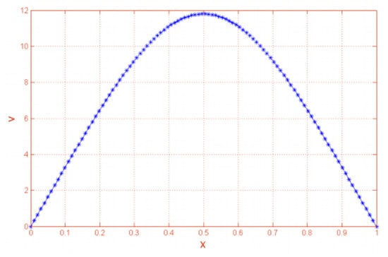
To discretize the above equation, we divide the interval $[0,1]$ into n equal parts, with the length of each part being $h=1/n$ and the coordinate of each point being $x_i=ih$, for $i=0,1,2,\dots ,n$. A second-order finite difference discretization of Equation (46) results in the following set of non-linear equations

$$F(\mathbf{v}):=\left\{\begin{array}{c}{v}_{i-1}+h^2{v}_i^2-2v_i+v_{i+1}=0\\ \mathit{for}i=1,2,\dots ,(n-1)\mathit{and}\mathit{from}(46)v_0=v_n=0\end{array},\right.$$

(47)

where $\mathbf{v}={[v_1,v_2,\dots ,v_{(n-1)}]}^{\mathrm{T}}$. For the above system of non-linear equations, we provide the Fréchet derivative

$$F^{\prime }(\mathbf{v})=\left[\begin{array}{ccccccc}{\displaystyle \frac{2v_1}{n^2}}-2& 1& 0& 0& \cdots & 0& 0\\ 1& {\displaystyle \frac{2v_2}{n^2}}-2& 1& 0& \cdots & 0& 0\\ 0& 1& {\displaystyle \frac{2v_3}{n^2}}-2& 1& \cdots & 0& 0\\ ⋮& ⋮& ⋮& ⋮& \cdots & ⋮& ⋮\\ 0& 0& 0& 0& \cdots & 1& {\displaystyle \frac{2v_{(n-1)}}{n^2}}-2\end{array}\right].$$

Let $n=101$ and $x_0={[5,5,\dots ,5]}^{\mathrm{T}}$. To solve the linear systems (step 1 and step 2 in the method (47)), we employ the MatLab routine “linsolve”, which uses LU factorization with partial pivoting. We define the initial guess to be $x_0=linspace(0,12,100)$. Figure 1 plots our numerical solution.

Example 7.

Radius Comparison Suppose that the motion of an object in three dimensions is governed by the system of differential equations

$$\begin{array}{c}{F}_1^{\prime }(x)-F_1(x)-1=0,\hfill \\ F_2^{\prime }(y)-(e-1)y-1=0,\hfill \\ F_3^{\prime }(z)-1=0,\hfill \end{array}$$

(48)

with $x,y,z\in D$ for $F_1(0)=F_2(0)=F_3(0)=0$. Then, the solution of the system is given, for $v={(x,y,z)}^T$, by the function $F:=(F_1,F_2,F_3):D\to {\mathbb{R}}^3$, defined by

$$F(v)={\left(e^x-1,\frac{e-1}{2}{y}^2+y,z\right)}^T.$$

Then, for $x^{*}={(0,0,0)}^T$, we have

$$L_0=e-1<L=e^{{\displaystyle \frac{1}{e-1}}}<L_1=e.$$

Notice that (41) holds. Hence, (29) holds as a strict inequality. In particular, we have, from (22), (23), and (27), that

$$r_1=0.245253\dots ,\overline{r^{*}}=0.324947\dots ,r^{*}=0.382692\dots .$$

Thus, we have improved the previous results.

4. Conclusions

Generalized Newton–Mysovskii-type majorant convergence results have been introduced in this paper. Special cases of the majorant functions involved lead to conditions considered by other authors [4,7,9,12,21,22]. It turns out that, although the conditions are more general, they are also more flexible, leading to some advantages; moreover, without any additional computational effort. Hence, we have extended the applicability of Newton’s method in cases not covered before. This paper paves the way for future research involving other iterative procedures involving inverses of linear operators.

References

- Argyros, I.K.; Hilout, S. Weaker conditions for the convergence of Newton’s method. J. Complex. 2012, 28, 364–387. [Google Scholar] [CrossRef]
- Argyros, I.K.; Magreñán, Á.A. On the convergence of an optimal fourth-order family of methods and its dynamics. Appl. Math. Comput. 2015, 252, 336–346. [Google Scholar] [CrossRef]
- Argyros, I.K.; González, D. Local convergence for an improved Jarratt-type method in Banach space. Int. J. Artif. Intell. Interact. Multimed. 2015, 3, 20–25. [Google Scholar] [CrossRef][Green Version]
- Deuflhard, P. Newton Methods for Nonlinear Problems: Affine Invariance and Adaptive Algorithms; Springer: Berlin/Heidelberg, Germany, 2011. [Google Scholar]
- Ferreira, O.P. Local convergence of Newton’s method in Banach space from the viewpoint of the majorant principle. IMA J. Numer. Anal. 2009, 29, 746–759. [Google Scholar] [CrossRef]
- Hernández, M.A.; Salanova, M.A. Modification of the Kantorovich assumptions for semilocal convergence of the Chebyshev method. J. Comput. Appl. Math. 2000, 126, 131–143. [Google Scholar]
- Kantorovich, L.V.; Akilov, G.P. Functional Analysis; Pergamon Press: Oxford, UK, 1982. [Google Scholar]
- Kou, J.S.; Li, Y.T.; Wang, X.H. A modification of Newton method with third-order convergence. Appl. Math. Comput. 2006, 181, 1106–1111. [Google Scholar] [CrossRef]
- Proinov, P.D. General local convergence theory for a class of iterative processes and its applications to Newton’s method. J. Complex. 2009, 25, 38–62. [Google Scholar] [CrossRef]
- Amat, S.; Busquier, S. Third order methods under Kantorovich conditions. J. Math. Anal. Appl. 2007, 336, 243–261. [Google Scholar] [CrossRef]
- Amat, S.; Bermúdez, C.; Busquier, S.; Plaza, S. On a third-order Newton-type method free of bilinear operators. Numer. Linear Algebra Appl. 2010, 17, 639–653. [Google Scholar] [CrossRef]
- Argyros, I.K. Computational Theory of Iterative Methods; Chui, C.K., Wuytack, L., Eds.; Studies in Computational Mathematics; Elsevier Publ. Co.: New York, NY, USA, 2007; Volume 15. [Google Scholar]
- Argyros, I.K. A semilocal convergence analysis for directional Newton methods. Math. Comput. 2011, 80, 327–343. [Google Scholar] [CrossRef]
- Argyros, I.K.; Hilout, S. Computational Methods in Nonlinear Analysis: Efficient Algorithms, Fixed Point Theory and Applications; World Scientific: Singapore, 2013. [Google Scholar]
- Argyros, I.K.; George, S. Ball Convergence for Steffensen-type Fourth-order Methods. Int. J. Artif. Intell. Interact. Multimed. 2015, 3, 37–42. [Google Scholar] [CrossRef][Green Version]
- Ezquerro, J.A.; Hernández, M.A. Recurrence relations for Chebyshev-type methods. Appl. Math. Optim. 2000, 41, 227–236. [Google Scholar] [CrossRef]
- Ezquerro, J.A.; Hernández, M.A. Third-order iterative methods for operators with bounded second derivative. J. Comput. Math. Appl. 1997, 82, 171–183. [Google Scholar]
- Ezquerro, J.A.; Hernández, M.A. On the R-order of the Halley method. J. Math. Anal. Appl. 2005, 303, 591–601. [Google Scholar] [CrossRef]
- Gopalan, V.B.; Seader, J.D. Application of interval Newton’s method to chemical engineering problems. Reliab. Comput. 1995, 1, 215–223. [Google Scholar]
- Gutiérrez, J.A.; Magreñán, Á.A.; Romero, N. On the semilocal convergence of Newton Kantorovich method under center-Lipschitz conditions. Appl. Math. Comput. 2013, 221, 79–88. [Google Scholar]
- Ortega, L.M.; Rheinboldt, W.C. Iterative Solution of Nonlinear Equations in Several Variables; Academic Press: New York, NY, USA, 1970. [Google Scholar]
- Potra, F.A.; Pták, V. Nondiscrete Induction and Iterative Processes; Research Notes in Mathematics; Pitman: Boston, MA, USA, 1984; Volume 103. [Google Scholar]
- Rheinboldt, W.C. An adaptive continuation process for solving systems of nonlinear equations. Banach Cent. Publ. 1977, 3, 129–142. [Google Scholar] [CrossRef]
- Traub, J.F. Iterative Methods for the Solution of Equations; Prentice-Hall Series in Automatic Computation; Prentice-Hall: Englewood Cliffs, NJ, USA, 1964. [Google Scholar]
- Smale, S. Newton’s method estimates from data at one point. In The Merging of Disciplines: New Directions in Pure, Applied, and Computational Mathematics; Springer: New York, NY, USA, 1986; pp. 185–196. [Google Scholar]
- Wang, X. Convergence of Newton’s method and uniqueness of the solution of equations in Banach space. IMA J. Numer. Anal. 2000, 20, 123–134. [Google Scholar] [CrossRef]
- Shacham, M. An improved memory method for the solution of a nonlinear equation. Chem. Eng. Sci. 1989, 44, 1495–1501. [Google Scholar] [CrossRef]
© 2019 by the authors. Licensee MDPI, Basel, Switzerland. This article is an open access article distributed under the terms and conditions of the Creative Commons Attribution (CC BY) license (http://creativecommons.org/licenses/by/4.0/).