Abstract
For the approximation of stiff systems of ODEs arising from chemistry kinetics, implicit integrators emerge as good candidates. This paper proposes a variational approach for this type of systems. In addition to introducing the technique, we present its most basic properties and test its numerical performance through some experiments. The main advantage with respect to other implicit methods is that our approach has a global convergence. The other approaches need to ensure convergence of the iterative scheme used to approximate the associated nonlinear equations that appear for the implicitness. Notice that these iterative methods, for these nonlinear equations, have bounded basins of attraction.
1. Introduction
We start with the following stiff differential problem:
Due to its stiffness, it is convenient to use implicit Runge-Kutta methods for the time integration step. The error analysis and the existence and uniqueness of the solution obtained through the Runge-Kutta method were analyzed in [1,2]. However, a difficulty appeared related to the approximation of the nonlinear Runge-Kutta equations by iterative methods [2], since we need to find good initial guesses. We will point out these difficulties in the Motivation Section.
The variational approach that we will use is based on the error functional:
that will be minimized among the absolutely-continuous path with . Note that if is finite for one such path x, then automatically, is square integrable. The error functional in (1) is associated with the original problem in a natural way: it only has a local minimum that is the solution of the problem. This property will imply the global convergence of our approach based on optimality conditions and minimization schemes like (steepest) descent methods. We only need to approximate linear problems; therefore, we can use the well-developed theory of the convergence of Runge-Kutta methods for stiff linear problems.
We will focus our attention on kinetic chemical reactions modeled through stiff differential equations. We will provide mathematical expressions for the reaction rate for problems where this rate is widely varying [3,4]. The main goal of this article is to test the variational approach exposed before to solve this kind of problems.
2. Motivation
One of the simplest stiff problems is the following linear test differential equation,
where is a complex number with Re . This equation is used to test the A-stability and imposes restrictions on the step size of explicit methods. In order to point out the problems with the initial guesses in the use of implicit methods, we will consider a nonlinear modification of the problem in (2). We consider the following nonlinear variation,
at . The explicit solution is given by the expression,
In order to solve this problem, we can consider the classical trapezoid rule,
The approximate solution of the problem in (2) obtained using this classical implementation is shown in Figure 1. To obtain these results, we have used (left) and 10,000 (right). We can see that the method provides a bad approximation when the stiffness of the problem increases, as shown in Figure 1 on the right. This is due to the fact that the initial guess is outside of the basin of attraction of Newton’s method [1]. However, looking at Figure 2, we can see that the variational method converges in the two considered cases.
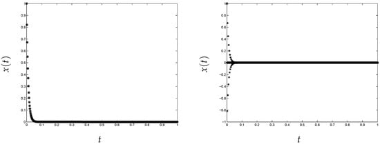
Figure 1.
Classical implementation of the trapezoid rule. Nonlinear test problem (“o”, original; “*”, approximation). (left) and (right) 10,000.
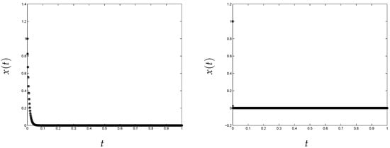
Figure 2.
Variational approach, nonlinear test problem (“o”, original; “*”, approximation). (left) and (right) 10,000.
3. Some Theoretical Analysis
One initial assumption that we must make about is its smoothness, so that is continuous. We will also assume global Lipschitzianity with Lipschitz constant (). Moreover, we will suppose that for every positive and small , there is a constant so that,
This regularity comes from the relation of our approach with optimality. On the other hand, these properties are verified for most of the important problems in chemistry kinetics.
The next theorem is a local existence result. Fortunately, if the function f verifies the hypotheses globally, applying this theorem to successively smaller intervals, we can derive a global strong convergence result.
Theorem 1.
Our iterative procedure , starting from any initial approximation , where:
converges strongly in and in to the unique solution of the original problem.
All the mathematical models considered in this work will verify the theoretical hypotheses since they will have both gradients and Hessians bounded.
Sketch of the proof:
We start with any initial approximation , for instance for all t, or . In order to reduce the error finding a descent direction, we compute the Gâteaux derivative of E in (1) at a given x in the direction y with . Namely,
In particular, we can propose to choose y such that,
This way it is clear that , and the (local) decrease of the error is of the size . Finding y requires solving the above linear problem. In some sense, this is like a Newton method. Through an induction process, we obtain the proof of the theorem. The complete proof of Theorem 1 can be found in [5]. □
4. Some Numerical Examples
In this section, we introduce some well-known chemical problems and apply our iterative scheme in order to obtain an approximation of the solution and to show the efficiency of the new method. The models are: the Robertson problem, the chemical Akzo Nobel problem, and the Hires problem. For the three models, our approach is convergent. Indeed, we have:
Corollary 1.
The three models (Robertson, chemical Akzo Nobel, and Hires) verify the hypotheses of Theorem 1.
Proof.
The three models considered in this section verify the theoretical hypotheses of the variational approach. Two of them are quadratic polynomials that have a constant Hessian, and the third is based on concentrations (all positive and bounded), in monomials and square roots. Therefore, all are sufficiently differentiable with bounded gradients and Hessians. □
In particular, the user can consider the variational method as a black box with theoretical guarantees. This is not the case of other approaches, like implicit Runge-Kutta, where only numerical evidence is presented. For a more general context, of the chemistry kinetics and its applications, we refer to [6].
The choice of initial conditions when integrating systems of ODEs is usually not trivial, especially when the equations are stiff, and hence, the solution is not easily predictable. Therefore, the introduction of a new method that, under reasonable hypotheses, allows for a global convergence is rather important in our opinion. The figures correspond to the approximation of our method using a stopping criterion when the error functional is smaller than , and the global convergence of our approach ensures the good approximation to the solution. In fact, our methods can be used to check the existence of a solution, since the method only diverges basically when the problem has no solution. In any case, the values and the plots are those expected for these problems.
4.1. Robertson Problem
The following chemical reaction process was introduced by Robertson in 1966 [7]:
The problem consists of three equations where , , and represent the rate constants and A, B, and C are the chemical species involved.
Under some conditions and applying the mass action law for the rate functions, the following mathematical model, which consists of a stiff system of three non-linear ordinary differential equations, is obtained,
In the previous system, , and were the concentrations of the chemical species A, B, and C, respectively. The initial values at time can be represented by . The values of the constants used in the test were , , and , and the initial concentrations were , , and . The time interval considered was . The stiffness of this problem is due to the large difference between the kinetic constants , which produce a very quick initial transient, as can be seen in Figure 3. The convergence of the method has been theoretically proven in [5]. In Figure 3, it is shown that the method converges and approximates well the solution of the Robertson problem. The numerical value of the solution for the three components , , of the Robertson problem at , using the variational method, can be seen in Table 1.
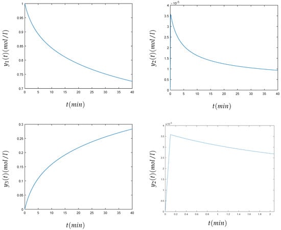
Figure 3.
Numerical solution of the concentrations (top left), (top right), and (bottom left) and a zoom of the transient around the origin of (bottom right) of the Robertson problem (3).

Table 1.
Results of the Robertson problem at .
4.2. Chemical Akzo Nobel Problem
This problem arose in Akzo Nobel Central Research (The Netherlands) [8]. The problem describes a chemical process, in which two species, FLBand ZLU, are mixed, while carbon dioxide is continuously added. The resulting species of importance is ZLA. The names of the different chemical species are fictitious due to the commercial competition in this field. The chemical reaction scheme is the following,
represents the constant of equilibrium of the last equation and has the expression,
Brackets represent concentrations. The velocities of the previous chemical equations are given respectively by:
defines the inflow of oxygen per unit volume and is given by:
where denotes the mass transfer coefficient, H is the Henry constant, and represents the partial pressure of oxygen and is considered independent of . , , , , K, , H, and are constant parameters. The mathematical model consists of a stiff system of six non-linear ordinary differential equations.
where the auxiliary variables and are:
The values of the parameters were , , , , , , . Initially, 0.44 mol/liter of FLB were mixed with 0.007 mol/liter of ZHU. At the beginning, the carbon dioxide had a concentration of 0.00123 mol/liter. The time of simulation was 180 minutes. The relation between chemical and mathematical formulation was that the concentration of the different components in chemical formulation , , , , , was respectively , …, in the mathematical formulation. The method was able to approximate the solution of this stiff problem. The convergence of the method can be seen in Figure 4. Table 2 shows the numerical solution of the components of the chemical Akzo Nobel problem , , , , , , at , when the variational method is used.
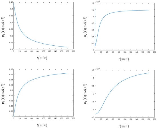
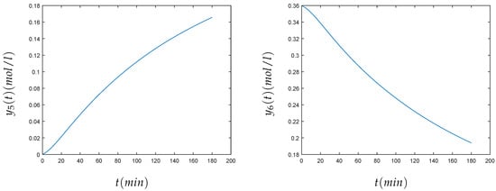
Figure 4.
Numerical solution of the concentrations (top left), (top right), (center left), (center right), (bottom left), and (bottom right) of the chemical Akzo Nobel problem (4) for min.
Table 2.
Results of the chemical Akzo Nobel problem at .
4.3. Hires Problem
Schäfer introduced this problem in 1975 [9]. It represents the high irradiance response (HIRES) of photomorphogenesis on the basis of the phytochrome. The chemical reactions have eight reactants. The problem can be formulated mathematically through a stiff system of eight non-linear differential equations.
The initial values were given by the vector . The end points of the time interval for each component have been arbitrarily chosen, as can be seen in the numerical results (Figure 5). For the components , , , , and , we have chosen the interval , and for the components and , we have chosen the interval . The problem has eight components, and it may be considered as a large number of components. In this case, the method also converges to the solution sought; see Figure 5. The numerical value of the solution for the eight components , , , , at and , at of the Hires problem, using the variational method, can be seen in Table 3.
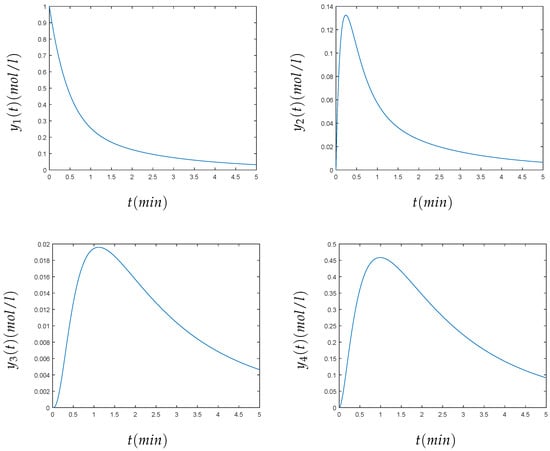
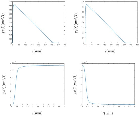
Figure 5.
From left to right and top to bottom, we present the numerical solution of the HIRES problem for min for the concentrations , , , , , and for min for and .
Table 3.
Results of the Hires problem at for , , , , , and at for and .
5. Conclusions
In stiff systems of ODEs, the restriction of the time step becomes severe, particularly when the simulation time is large. In this paper, the new variational method proposed has been successfully applied to several initial value problems arising from chemical reactions composed of large systems of stiff ODEs. Moreover, the variational method has the advantage of never getting stuck at local minima. It always converges to the solution regardless of the initialization. This is an important improvement over the methods that need an initialization that is close to the solution of the problem like the implicit Runge-Kutta methods.
Author Contributions
These authors contributed equally to this work.
Funding
Proyecto financiado por la Comunidad Autónoma de la Región de Murcia a través de la convocatoria de Ayudas a proyectos para el desarrollo de investigación científica y técnica por grupos competitivos, incluida en el Programa Regional de Fomento de la Investigación Científica y Técnica (Plan de Actuación 2018) de la Fundación Séneca-Agencia de Ciencia y Tecnología de la Región de Murcia 20928/PI/18, MTM2015-64382-P (MINECO/FEDER).
Conflicts of Interest
The authors declare no conflict of interest.
References
- Auzinger, W.; Frank, R.; Kirlinger, G. An extension of B-convergence for Runge-Kutta methods. Appl. Numer. Math. 1992, 9, 91–109. [Google Scholar] [CrossRef]
- Hairer, E.; Wanner, G. Solving Ordinary Differential Equations II: Stiff and Differential Algebraic Problems; Springer: Berlin, Germany, 1991. [Google Scholar]
- Brasseur, G.; Jacob, D. Numerical Methods for Chemical Systems. In Modeling of Atmospheric Chemistry; Cambridge University Press: Cambridge, UK, 2017; pp. 253–274. [Google Scholar]
- Rué, P.; Villà-Freixa, J.; Burrage, K. Simulation methods with extended stability for stiff biochemical Kinetics. BMC Syst. Biol. 2010, 4, 110. [Google Scholar] [CrossRef] [PubMed]
- Legaz, M.J. Approximation of Differential Equations Through a New Variational Technique and Applications. 2012. Available online: http://repositorio.upct.es/handle/10317/3740 (accessed on 19 March 2019).
- Dos Santos, M.A.F. From continuous-time random walks to controlled-diffusion reaction. J. Stat. Mech. 2019, 033214. [Google Scholar] [CrossRef]
- Robertson, H.H. The solution of a set of reaction rate equations. In Numerical Analysis: An Introduction; Academic Press: London, UK, 1966. [Google Scholar]
- CBS-Reaction-Meeting Köln. Br/ARLO-CRC. Handouts, 1993. Available online: https://es.linkedin.com/company/akzo-nobel-central-research (accessed on 19 April 2019).
- Schäfer, E. A new approach to explain the ’high irradiance responses’ of photomorphogenesis on the basis of phytochrome. J. Math. Biol. 1975, 2, 41–56. [Google Scholar] [CrossRef]
© 2019 by the authors. Licensee MDPI, Basel, Switzerland. This article is an open access article distributed under the terms and conditions of the Creative Commons Attribution (CC BY) license (http://creativecommons.org/licenses/by/4.0/).