Skew-Reflected-Gompertz Information Quantifiers with Application to Sea Surface Temperature Records

Abstract

The Skew-Reflected-Gompertz (SRG) distribution, introduced by Hosseinzadeh et al. (J. Comput. Appl. Math. (2019) 349, 132–141), produces two-piece asymmetric behavior of the Gompertz (GZ) distribution, which extends the positive to a whole dominion by an extra parameter. The SRG distribution also permits a better fit than its well-known classical competitors, namely the skew-normal and epsilon-skew-normal distributions, for data with a high presence of skewness. In this paper, we study information quantifiers such as Shannon and Rényi entropies, and Kullback–Leibler divergence in terms of exact expressions of GZ information measures. We find the asymptotic test useful to compare two SRG-distributed samples. Finally, as a real-world data example, we apply these results to South Pacific sea surface temperature records.

1. Introduction

The Skew-Reflected-Gompertz (SRG) distribution was recently introduced by [1] and corresponds to an extension of the Gompertz distribution [2], named after Benjamin Gompertz (1779–1865). It extends the positive dominion ${\mathbb{R}}_{+}$ to the whole of $\mathbb{R}$ by an extra parameter, $\epsilon$, $-1<\epsilon <1$, and produces two-piece asymmetric behavior of Gompertz (GZ) density. The SRG distribution has as particular cases the Reflected-GZ and GZ distributions, when $\epsilon \to 1$ and $\epsilon \to -1$, respectively. The SRG distribution family can also represent a suitable competitor against the skew-normal (SN, [3]) and epsilon-skew-normal (ESN, [4]) distributions as a way to fit asymmetrical datasets. Indeed, refs. [5,6] dealt with the frequentist and Bayesian inferences of ESN distribution. Contributions by [1] provided probability density function (pdf), cumulative distribution function (cdf), quantile function, moment-generating function (MGF), stochastic representation, the Expectation-Maximization (EM) algorithm for SRG parameter estimates and the Fisher information matrix (FIM).

Moreover, several recent investigations confirmed the usefulness of entropic quantifiers in the study of asymmetric distributions [3,7,8] and their applications to topics such as thermal wake [9], marine fish biology [3,8], sea surface temperature (SST), relative humidity measured in the Atlantic Ocean [10], and more. We build on the study of [3], which developed hypothesis testing for normality, i.e., if the shape parameter is close to zero. They considered the Kullback–Leibler (KL) divergence in terms of moments and cumulants of the modified SN distribution. Posteriorly, we consider a real-world data set of the anchovy condition factor for testing the shape parameter to decide if a food deficit produced by environmental conditions such as El Niño exists [11].

This work arose from a motivation to tackle the problem of determining the adequate pdf of SST [9,10]. Indeed, probabilistic modelling of SST is key for accurate predictions [9]. Therefore, we propose that the SRG model based on two-piece distributions could be more suitable for interpreting annual bimodal and asymmetric SST data. We also considered the existent results of Shannon and Rényi entropies, and KL divergence for GZ distributions for developed entropic quantifiers for SRG distributions. Posteriorly, we considered SST along the South Pacific and Chilean coasts from 2012 to 2014 to illustrate our results. Specifically, we introduced hypothesis testing developed by [12] for the SRG distribution, which is useful to compare two data sets with bimodal and asymmetric behavior such as SST.

2. The Skew-Reflected-Gompertz Distribution

The Gompertz (GZ, [2]) distribution is a continuous probability distribution with the following pdf

$$\begin{array}{c}\hfill f\left(x\right|\sigma ,\eta )=\frac{\eta }{\sigma }{e}^{\frac{x}{\sigma }}{e}^{-\eta (e^{\frac{x}{\sigma }}-1)},x\ge 0,\end{array}$$

(1)

where $\sigma >0$ and $\eta >0$ are the scale and shape parameters, respectively, and are denoted by $X\sim GZ(\sigma ,\eta )$. The mean and variance of X are

$$\begin{array}{ccc}\hfill E\left(X\right)& =& \sigma e^{\eta }Ei(-\eta ),\hfill \\ \hfill Var\left(X\right)& =& {\sigma }^2{e}^{\eta }\tau ,\hfill \end{array}$$

(2)

respectively; where $Ei\left(z\right)={\int }_{-z}^{\infty }\frac{e^{-u}}{u}du$, $\tau =-2\eta F(-\eta )+{\gamma }^2+\frac{{\pi }^2}{6}+2\gamma log\eta +{(log\eta )}^2-e^{\eta }{\left[Ei(-\eta )\right]}^2$, $\gamma =0.5772156649$ is the Euler constant and

$$F\left(z\right)=\sum _{k=0}^{+\infty }\frac{z^k}{k!{(k+1)}^3}.$$

The SRG distribution is an extension of the GZ proposed by [1]. If Y follows, the SRG distribution is denoted by $Y\sim \mathrm{SRG}(\mu ,\sigma ,\eta ,\epsilon )$ and has pdf

$$\begin{array}{c}\hfill g\left(y\right|\mu ,\sigma ,\eta ,\epsilon )=\left\{\begin{array}{cc}\frac{1}{2}f\left(\frac{\mu -y}{1+\epsilon }|\sigma ,\eta \right),\hfill & y\le \mu ,\hfill \\ \frac{1}{2}f\left(\frac{y-\mu }{1-\epsilon }|\sigma ,\eta \right),\hfill & y>\mu ,\hfill \end{array}\right.\end{array}$$

(3)

where $\mu \in \mathbb{R}$ is the location parameter and $\epsilon \in (-1,1)$ is the slant parameter. Note that SRG is the GZ distribution when $\mu =0$ and $\epsilon \to -1$, GZ distribution with negative support when $\epsilon \to 1$, and Reflected-GZ distribution when $\epsilon =0$. Also, the Reflected-GZ distribution corresponds to a particular case of a more general class of two-piece asymmetric distributions proposed by [13,14]. The mean, variance and MGF of Y are

$$\begin{array}{ccc}\hfill E\left(Y\right)& =& \mu -2\epsilon \sigma e^{\eta }Ei(-\eta ),\hfill \\ \hfill Var\left(Y\right)& =& {\sigma }^2\{\tau e^{\eta }+2(1-{\epsilon }^2)e^{2\eta }{\left[Ei(-\eta )\right]}^2\},\hfill \\ \hfill M_Y\left(t\right)& =& \frac{1}{2}\eta e^{\eta +\mu t}[(1-\epsilon ){ϝ}_{-\sigma t}\left(\eta \right)+(1+\epsilon ){ϝ}_{\sigma t}\left(\eta \right)],\hfill \end{array}$$

(4)

respectively; where ${ϝ}_s\left(z\right)={\int }_1^{\infty }{v}^{s+1}{e}^{-vz}dv$. Jafari et al. [15] provide the MGF of X using expansion series. However, (4) is considered a clearer expression that depends only on integral ${ϝ}_s\left(z\right)$. See Section 4.1 for some details of the MLE EM-based algorithm related to SRG parameters.

According to [1], the SRG distribution can be re-parametrized in terms of GZ and Reflected-GZ distributions as

$$\begin{array}{c}\hfill g\left(y\right|\mu ,{\sigma }_{+},{\sigma }_{-},\eta )=p_{1}f(\mu -y|{\sigma }_{+},\eta )I_{(-\infty ,\mu ]}\left(y\right)+p_{2}f(y-\mu |{\sigma }_{-},\eta )I_{(\mu ,+\infty )}\left(y\right),\end{array}$$

(5)

where ${\sigma }_{\pm }=\sigma (1\pm \epsilon )$, $p_1+p_2=1$, and $p_1={\sigma }_{+}/({\sigma }_{+}+{\sigma }_{-})=(1+\epsilon )/2$. Let $\mathbf{Y}={(Y_1,\dots ,Y_n)}^{\top }$ be an i.i.d sample from the SRG distribution with parameters $(\mu ,{\sigma }_{\pm },\eta )$ and latent vectors $\mathbf{Z}=({\mathbf{Z}}_1,\dots ,{\mathbf{Z}}_n)$, thus (5) can be equivalently represented as ${(-1)}^j(Y_i-\mu )|Z_{ij}=1\sim GZ({\sigma }_{\pm },\eta )$, $i=1,\dots ,n$, $j=1,2$, where ${\mathbf{Z}}_i={(Z_{i1},Z_{i2})}^{\top }\sim Mult(1,p_1,p_2)$ is a multinomial vector, $P(Z_{i1}=z_{i1},Z_{i2}=z_{i2})=p_1^{z_{i1}}{p}_2^{z_{i2}}$, $z_{ij}=\{0,1\}$, and $z_{i1}+z_{i2}=1$. Given that $P(Z_{i1}=1)=P(Z_{i1}=1,Z_{ik}=0;\forall j\ne k)$, the complete log-likelihood function is

$$\begin{array}{ccc}\hfill \ell (\mu ,{\sigma }_{+},{\sigma }_{-},\eta |\mathbf{Y},\mathbf{Z})& =& -nlog\left(2\sigma \right)+n(\eta +log\eta )\hfill \\ & & +\sum _{i=1}^n\left[z_{i1}\left(\frac{\mu -y_i}{{\sigma }_{+}}-\eta e^{\frac{\mu -y_i}{{\sigma }_{+}}}\right)+z_{i2}\left(\frac{y_i-\mu }{{\sigma }_{-}}-\eta e^{\frac{y_i-\mu }{{\sigma }_{-}}}\right)\right].\hfill \end{array}$$

(6)

Conditional expectations of latent variables ${\mathbf{Z}}_i$ are given by

$$\begin{array}{ccc}\hfill {\widehat{z}}_{i1}& =& E\left[Z_{i1}\right|\widehat{\mu },{\widehat{\sigma }}_{+},{\widehat{\sigma }}_{-},y_i]={\widehat{p}}_1\frac{f(\widehat{\mu }-y_i|{\widehat{\sigma }}_{+},\widehat{\eta })}{g\left(y_i\right|\widehat{\mu },{\widehat{\sigma }}_{+},{\widehat{\sigma }}_{-},\widehat{\eta })}{I}_{(-\infty ,\widehat{\mu }]}\left(y_i\right),\hfill \end{array}$$

(7)

$$\begin{array}{ccc}\hfill {\widehat{z}}_{i2}& =& 1-{\widehat{z}}_{i1},i=1,\dots ,n.\hfill \end{array}$$

(8)

The E- and M-steps on the $(k+1)$th iteration of the EM algorithm are

• E-step. From (6)–(8), we have

  $$\begin{array}{ccc}\hfill Q(\mu ,{\sigma }_{+},{\sigma }_{-},\eta |{\mu }^{\left(k\right)},{\sigma }_{+}^{\left(k\right)},{\sigma }_{-}^{\left(k\right)},{\eta }^{\left(k\right)})& =& E[\ell (\mu ,{\sigma }_{+},{\sigma }_{-},\eta |\mathbf{Y},\mathbf{Z})|{\mu }^{\left(k\right)},{\sigma }_{+}^{\left(k\right)},{\sigma }_{-}^{\left(k\right)},{\eta }^{\left(k\right)}]\hfill \\ & =& -nlog\left(2\sigma \right)+n(\eta +log\eta )\hfill \\ & & +\sum _{i=1}^n\left[{\widehat{z}}_{i1}^{\left(k\right)}\left(\frac{\mu -y_i}{{\sigma }_{+}}-\eta e^{\frac{\mu -y_i}{{\sigma }_{+}}}\right)+{\widehat{z}}_{i2}^{\left(k\right)}\left(\frac{y_i-\mu }{{\sigma }_{-}}-\eta e^{\frac{y_i-\mu }{{\sigma }_{-}}}\right)\right].\hfill \end{array}$$

  and
• M-step. Update ${\sigma }_{\pm }$, by solving the following equation

  $$\sum _{i=1}^n{\widehat{z}}_{ij}^{\left(k\right)}\left({\eta }^{\left(k\right)}\frac{|y_i-{\mu }^{\left(k\right)}|}{{\sigma }_{\pm }^2}{e}^{\frac{|y_i-{\mu }^{\left(k\right)}|}{{\sigma }_{\pm }}}-\frac{|y_i-{\mu }^{\left(k\right)}|}{{\sigma }_{\pm }^2}\right)=\frac{n}{2\sigma }.$$

Update $\mu$ by solving the following equation

$${\widehat{\mu }}^{(k+1)}={\mathrm{argmax}}_{\mu }\sum _{i=1}^n\left\{{\widehat{z}}_{i1}^{\left(k\right)}\left(\frac{\mu -y_i}{{\widehat{\sigma }}_{+}^{(k+1)}}-\eta e^{\frac{\mu -y_i}{{\widehat{\sigma }}_{+}^{(k+1)}}}\right)+{\widehat{z}}_{i2}^{\left(k\right)}\left(\frac{\mu -y_i}{{\widehat{\sigma }}_{-}^{(k+1)}}-\eta e^{\frac{\mu -y_i}{{\widehat{\sigma }}_{-}^{(k+1)}}}\right)\right\}.$$

Update $\eta$ by

$$\widehat{\eta }=n{\left(\sum _{i=1}^n\left\{{\widehat{z}}_{i1}^{\left(k\right)}{e}^{\frac{\mu -y_i}{{\widehat{\sigma }}_{+}^{(k+1)}}}+{\widehat{z}}_{i2}^{\left(k\right)}{e}^{\frac{\mu -y_i}{{\widehat{\sigma }}_{-}^{(k+1)}}}\right\}\right)}^{-1}.$$

The EM-algorithm must be iterated until the sufficient convergence rule is satisfied:

$$\parallel ({\widehat{\mu }}^{(k+1)},{\widehat{\sigma }}_{+}^{(k+1)},{\widehat{\sigma }}_{-}^{(k+1)},{\widehat{\eta }}^{(k+1)})-({\widehat{\mu }}^{\left(k\right)},{\widehat{\sigma }}_{+}^{\left(k\right)},{\widehat{\sigma }}_{-}^{\left(k\right)},{\widehat{\eta }}^{\left(k\right)})\parallel <\tau ,$$

for a tolerance $\tau$ close to zero. The FIM for standard deviations of MLEs $(\widehat{\mu },\widehat{\sigma },\widehat{\eta },\widehat{\epsilon })$ and additional details of the EM-algorithm are described in [1].

3. Entropic Quantifiers

In the next section, we present the main results of entropic quantifiers for SRG distribution.

3.1. Shannon Entropy

The Shannon entropy (SE), introduced by [16] in the context of univariate continuous distributions, quantifies the information contained in a random variable X with pdf $f\left(x\right)$ through the expression

$$\begin{array}{c}\hfill H\left(X\right)=-{\int }_{-\infty }^{+\infty }f\left(x\right)logf\left(x\right)dx.\end{array}$$

(9)

The SE concept is attributed to the uncertainty of the information presented in X [17]. Propositions 1 and 2 present the SE for GZ and SRG distributions, respectively.

Proposition 1.

[15]. The SE of $X\sim GZ(\sigma ,\eta )$ is

$$H\left(X\right)=log\left\{\frac{B(1,1)}{\eta }\right\}-\sigma \eta -\frac{E\left(X\right)}{\sigma }+\sigma \eta M_X\left({\sigma }^{-1}\right),$$

where $B(·,·)$ is the usual Beta function and $E\left(X\right)$ is given in (2).

Substituting $\mu =0$ and $\epsilon =-1$ into (4) (i.e., reducing SRG to its special case GZ), we obtain $M_X({\sigma }^{-1})=\eta e^{\eta }{ϝ}_{-1}\left(\eta \right)=1$. Therefore, $H\left(X\right)$ in Proposition 1 is reduced to

$$\begin{array}{c}\hfill H\left(X\right)=-log\eta -e^{\eta }{E}_i(-\eta ),\end{array}$$

(10)

i.e., the SE of the GZ random variable only depends on shape parameter $\eta$.

Proposition 2.

The SE of $Y\sim SRG(\mu ,\sigma ,\eta ,\epsilon )$ is

$$H\left(Y\right)=\frac{1+\epsilon }{2}\left\{H\left(X_{+\epsilon }\right)-log\left(\frac{1+\epsilon }{2}\right)\right\}+\frac{1-\epsilon }{2}\left\{H\left(X_{-\epsilon }\right)-log\left(\frac{1-\epsilon }{2}\right)\right\},$$

where $X_{\pm \epsilon }\sim GZ(\sigma (1\pm \epsilon ),\eta )$ and $H\left(X_{\pm \epsilon }\right)$ are obtained using Proposition 1.

Proof. 

From (3) and (9), we obtained

$$\begin{array}{ccc}\hfill H\left(Y\right)& =& -{\int }_{-\infty }^{+\infty }g\left(y\right|\mu ,\sigma ,\eta ,\epsilon )logg\left(y\right|\mu ,\sigma ,\eta ,\epsilon )dy\hfill \\ & =& -\frac{1}{2}{\int }_0^{+\infty }f\left(\frac{x}{1+\epsilon }|\sigma ,\eta \right)log\left\{\frac{1}{2}f\left(\frac{x}{1+\epsilon }|\sigma ,\eta \right)\right\}dx\hfill \\ & & -\frac{1}{2}{\int }_0^{+\infty }f\left(\frac{x}{1-\epsilon }|\sigma ,\eta \right)log\left\{\frac{1}{2}f\left(\frac{x}{1-\epsilon }|\sigma ,\eta \right)\right\}dx\hfill \\ & =& -\frac{1}{2}{\int }_0^{+\infty }(1+\epsilon )f\left(x\right|\sigma (1+\epsilon ),\eta )log\left\{\frac{1+\epsilon }{2}f\left(x\right|\sigma (1+\epsilon ),\eta )\right\}dx\hfill \\ & & -\frac{1}{2}{\int }_0^{+\infty }(1-\epsilon )f\left(x\right|\sigma (1-\epsilon ),\eta )log\left\{\frac{1-\epsilon }{2}f\left(x\right|\sigma (1-\epsilon ),\eta )\right\}dx,\hfill \end{array}$$

which concludes the proof. □

From (10), given that $H\left(X_{\pm \epsilon }\right)$ only depends on shape parameter $\eta$, we obtain $H\left(X_{\pm \epsilon }\right)=H\left(X\right)$, and $H\left(Y\right)$ only depends on $\eta$ and $\epsilon$ parameters. Therefore,

$$\begin{array}{c}\hfill H\left(Y\right)=-log\eta -e^{\eta }{E}_i(-\eta )-\frac{1+\epsilon }{2}log\left(\frac{1+\epsilon }{2}\right)-\frac{1-\epsilon }{2}log\left(\frac{1-\epsilon }{2}\right).\end{array}$$

(11)

Figure 1 illustrates SE behavior for random variable Y. We observed that SE increases when $\eta$ decreases. For each $\eta$, SE is maximized and minimized at $\epsilon =0$ (Reflected-GZ) and $\epsilon \to -1$ (Truncated-GZ and GZ), respectively. More details appear in [3,8] for the SE expressions of other asymmetric distributions.

3.2. Rényi Entropy

The $\alpha$th-order Rényi entropy (RE), introduced by [18] in the context of univariate continuous distributions, extends the concept of SE information contained in a random variable X with pdf $f\left(x\right)$ through a level $\alpha$, $\alpha \in \mathbb{N}$, $\alpha >0$, and the expression

$$\begin{array}{c}\hfill R_{\alpha }\left(X\right)=\frac{1}{1-\alpha }log{\int }_{-\infty }^{+\infty }{\left[f\left(x\right)\right]}^{\alpha }dx.\end{array}$$

(12)

RE information can be negative and is ordered with respect to $\alpha$, i.e., $R_{{\alpha }_1}\left(X\right)\ge R_{{\alpha }_2}\left(X\right)$ for any ${\alpha }_1<{\alpha }_2$ (see, e.g., [7] and other properties of RE). From (12), the SE is obtained by the limit of $H\left(X\right)={lim}_{\alpha \to 1}{R}_{\alpha }\left(X\right)$ by applying l’Hôpital’s rule to $R_{\alpha }\left(X\right)$ with respect to $\alpha$ (see e.g., [7]). The RE of the GZ and SRG distributions is presented in Propositions 3 and 4, respectively.

Proposition 3.

[15,19]. The RE of $X\sim GZ(\sigma ,\eta )$ with $\alpha >1$, $\alpha \in \mathbb{N}$, is

$$R_{\alpha }\left(X\right)=-\frac{log\alpha }{1-\alpha }+log\frac{\eta }{\sigma }+\frac{1}{1-\alpha }log\left\{\sum _{j=0}^{\alpha -1}\left(\genfrac{}{}{0pt}{}{\alpha -1}{j}\right)\frac{\mathrm{\Gamma }(j+1)}{{\left(\alpha \eta \right)}^j}\right\},$$

where $\mathrm{\Gamma }\left(u\right)={\int }_0^{\infty }{t}^{u-1}{e}^{-t}dt$ is the gamma function.

Proposition 4.

The RE of $Y\sim SRG(\eta ,\epsilon )$ with $\alpha >1$, $\alpha \in \mathbb{N}$, is

$$R_{\alpha }\left(Y\right)=\frac{1}{1-\alpha }log\left\{{\left(\frac{1+\epsilon }{2}\right)}^{\alpha }{e}^{(1-\alpha )R_{\alpha }\left(X_{+\epsilon }\right)}+{\left(\frac{1-\epsilon }{2}\right)}^{\alpha }{e}^{(1-\alpha )R_{\alpha }\left(X_{-\epsilon }\right)}\right\},$$

where $X_{\pm \epsilon }\sim GZ(\sigma (1\pm \epsilon ),\eta )$ and $R_{\alpha }\left(X_{\pm \epsilon }\right)$ are obtained using Proposition 3.

Proof. 

From (3) and (12), we obtained

$$\begin{array}{ccc}\hfill R_{\alpha }\left(Y\right)& =& \frac{1}{1-\alpha }log{\int }_{-\infty }^{+\infty }{\left[g\left(y\right|\mu ,\sigma ,\eta ,\epsilon )\right]}^{\alpha }dy,\hfill \\ & =& \frac{1}{1-\alpha }log\left\{{\int }_0^{+\infty }{\left[\frac{1}{2}f\left(\frac{x}{1+\epsilon }|\sigma ,\eta \right)\right]}^{\alpha }dx+{\int }_0^{+\infty }{\left[\frac{1}{2}f\left(\frac{x}{1-\epsilon }|\sigma ,\eta \right)\right]}^{\alpha }dx\right\},\hfill \\ & =& \frac{1}{1-\alpha }log\left\{{\left(\frac{1+\epsilon }{2}\right)}^{\alpha }{\int }_0^{+\infty }{\left[f\left(x\right|\sigma (1+\epsilon ),\eta )\right]}^{\alpha }dx+{\left(\frac{1-\epsilon }{2}\right)}^{\alpha }{\int }_0^{+\infty }{\left[f\left(x\right|\sigma (1-\epsilon ),\eta )\right]}^{\alpha }dx\right\},\hfill \end{array}$$

which concludes the proof. □

Figure 2a illustrates the behavior of RE for random variable Y when $\alpha =2$ (quadratic RE). As in the SE case, we also observed that RE increases when $\eta$ decreases and reaches maximum and minimum at $\epsilon =0$ (Reflected-GZ) and $\epsilon \to -1$ (Truncated-GZ and GZ), respectively. When $\alpha =5$ (or $\alpha >2$) (see Figure 2b), RE decays faster than in the quadratic RE case as $\epsilon \to -1$. More details appear in [7] for the RE expressions of other asymmetric distributions.

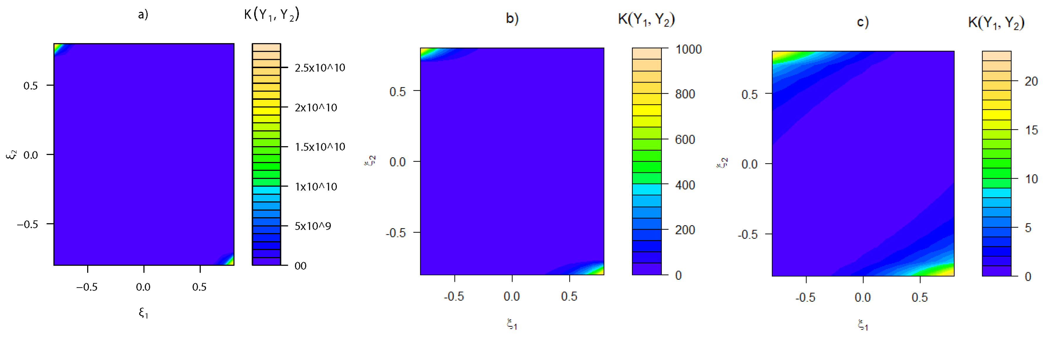
3.3. Kullback–Leibler Divergence

The Kullback–Leibler (KL) divergence introduced by [20] in the context of univariate continuous distributions, extends the concept of SE between two random variables $X_1$ and $X_2$ with pdfs $f_1\left(x_1\right)$ and $f_2\left(x_2\right)$, respectively, through the expression

$$\begin{array}{c}\hfill K(X_1,X_2)={\int }_{-\infty }^{+\infty }{f}_1\left(x\right)log\left\{\frac{f_1\left(x\right)}{f_2\left(x\right)}\right\}dx.\end{array}$$

(13)

The KL divergence measures the disparity between the pdfs of $X_1$ and $X_2$, and is non-negative, non-symmetric and zero only if $X_1=X_2$ in distribution. Also, the KL divergence does not satisfy the triangular inequality (see, e.g., [8,17] for other properties of KL and other divergences). The KL divergence for two GZ and two SRG distributions are presented in Propositions 5 and 6.

Proposition 5.

[21]. The KL divergence between $X_1\sim GZ({\sigma }_1,{\eta }_1)$ and $X_2\sim GZ({\sigma }_2,{\eta }_2)$ is

$$K(X_1,X_2)=log\left\{\frac{e^{{\eta }_1}{\sigma }_2{\eta }_1}{e^{{\eta }_2}{\sigma }_1{\eta }_2}\right\}+e^{{\eta }_1}\left[\left(\frac{{\sigma }_1}{{\sigma }_2}-1\right)E_i(-{\eta }_1)+\frac{{\eta }_2}{{\eta }_1^{{\sigma }_1/{\sigma }_2}}\mathrm{\Gamma }\left(\frac{{\sigma }_1}{{\sigma }_2}-1,{\eta }_1\right)\right]-({\eta }_1+1),$$

where $\mathrm{\Gamma }(u,v)={\int }_v^{\infty }{t}^{u-1}{e}^{-t}dt$ is the upper incomplete gamma function.

Proposition 6.

The KL divergence between $Y_1\sim SRG(0,{\sigma }_1,{\eta }_1,{\epsilon }_1)$ and $Y_2\sim SRG(0,{\sigma }_2,{\eta }_2,{\epsilon }_2)$ is

$$\begin{array}{ccc}\hfill K(Y_1,Y_2)& =& \frac{1+{\epsilon }_1}{2}\left[log\left\{\frac{1+{\epsilon }_1}{1+{\epsilon }_2}\right\}+K(X_{+{\epsilon }_1},X_{+{\epsilon }_2})\right]+\frac{1-{\epsilon }_1}{2}\left[log\left\{\frac{1-{\epsilon }_1}{1-{\epsilon }_2}\right\}+K(X_{-{\epsilon }_1},X_{-{\epsilon }_2})\right],\hfill \end{array}$$

where $X_{\pm {\epsilon }_i}\sim GZ({\sigma }_i(1\pm {\epsilon }_i),{\eta }_i)$, $i=1,2$, and $K(X_{\pm {\epsilon }_1},X_{\pm {\epsilon }_2})$ are obtained using Proposition 5.

Proof. 

From (3) and (13), we obtained

$$\begin{array}{ccc}\hfill K(Y_1,Y_2)& =& {\int }_{-\infty }^{+\infty }g\left(x\right|0,{\sigma }_1,{\eta }_1,{\epsilon }_1)log\left\{\frac{g\left(x\right|0,{\sigma }_1,{\eta }_1,{\epsilon }_1)}{g\left(x\right|0,{\sigma }_2,{\eta }_2,{\epsilon }_2)}\right\}dx,\hfill \\ & =& \frac{1}{2}{\int }_0^{+\infty }f\left(\frac{x}{1+{\epsilon }_1}|{\sigma }_1,{\eta }_1\right)log\left\{\frac{f\left(\frac{x}{1+{\epsilon }_1}|{\sigma }_1,{\eta }_1\right)}{f\left(\frac{x}{1+{\epsilon }_2}|{\sigma }_2,{\eta }_2\right)}\right\}dx\hfill \\ & & +\frac{1}{2}{\int }_0^{+\infty }f\left(\frac{x}{1-{\epsilon }_1}|{\sigma }_1,{\eta }_1\right)log\left\{\frac{f\left(\frac{x}{1-{\epsilon }_1}|{\sigma }_1,{\eta }_1\right)}{f\left(\frac{x}{1-{\epsilon }_2}|{\sigma }_2,{\eta }_2\right)}\right\}dx,\hfill \\ & =& \frac{1+{\epsilon }_1}{2}\left[log\left\{\frac{1+{\epsilon }_1}{1+{\epsilon }_2}\right\}+{\int }_0^{+\infty }f\left(x|{\sigma }_1(1+{\epsilon }_1),{\eta }_1\right)log\left\{\frac{f\left(x|{\sigma }_1(1+{\epsilon }_1),{\eta }_1\right)}{f\left(x|{\sigma }_2(1+{\epsilon }_2),{\eta }_2\right)}\right\}dx\right]\hfill \\ & & +\frac{1-{\epsilon }_1}{2}\left[log\left\{\frac{1-{\epsilon }_1}{1-{\epsilon }_2}\right\}+{\int }_0^{+\infty }f\left(x|{\sigma }_1(1-{\epsilon }_1),{\eta }_1\right)log\left\{\frac{f\left(x|{\sigma }_1(1-{\epsilon }_1),{\eta }_1\right)}{f\left(x|{\sigma }_2(1-{\epsilon }_2),{\eta }_2\right)}\right\}dx\right],\hfill \end{array}$$

which concludes the proof. □

More details appear in [3,8] for the KL divergence expressions of other asymmetric distributions. Using Proposition 6, the asymptotic KL divergence between $Y\sim \mathrm{SRG}(0,\sigma ,\eta ,\epsilon )$ and $X\sim \mathrm{GZ}(\sigma ,\eta )$ is

$$K(Y,X)\approx \frac{1+\epsilon }{2}\left[\underset{{\epsilon }_2\to -1}{lim}log\left(\frac{1+\epsilon }{1+{\epsilon }_2}\right)+K(X_{+\epsilon },X)\right]+\frac{1-\epsilon }{2}\left[log\left(\frac{1-\epsilon }{2}\right)+K(X_{-\epsilon },X)\right],$$

as ${\epsilon }_2\to -1$. However, we see that $log\left(\frac{1+\epsilon }{1+{\epsilon }_2}\right)=+\infty$ as ${\epsilon }_2\to -1$ and $K(Y,X)$ is not finite. However, from Proposition 6 the asymptotic KL divergence between $Y_1$ and $Y_2$ is

$$K(Y_1,Y_2)\approx K(X,Y)=log\left(\frac{2}{1-\epsilon }\right)+K(X,X_{-\epsilon }),$$

(14)

as ${\epsilon }_1\to -1$, where $X_{-\epsilon }\sim \mathrm{GZ}(\sigma (1-\epsilon ),\eta )$. Therefore, while $K(Y,X)$ is not finite, $K(X,Y)$ is finite and can be used to study the disparity of $\epsilon$ from −1. Thus, hypothesis testing for $H_0:\epsilon =-1$ can be addressed. Besides, we further study hypothesis testing for scale and shape parameters between two SRG distributions in Section 3.4. From (14), we also took that $K(Y_1,Y_2)\approx K(X,X_1)$ as $\epsilon \to -1$, with $X_1\sim \mathrm{GZ}(2\sigma ,\eta )$.

Figure 3 illustrates the KL divergence between two SRG distributions. We observed that for the critical points of $({\epsilon }_1,{\epsilon }_2)\to \{(-1,1);(1,-1)\}$, the KL divergence reaches the highest values and is close to zero in the other values [panels (a) and (b)]. For large $\eta$’s [panel (c)], the KL divergence is zero for a concentrated region of the dominion where ${\epsilon }_1={\epsilon }_2$.

All information quantifiers and the EM algorithm for SRG distribution were implemented in [22].

3.4. Asymptotic Test

Consider two independent samples of sizes $n_1$ and $n_2$ from $Y_1$ and $Y_2$, respectively; where $\mathbf{\theta },{\mathbf{\theta }}^{\prime }\in \mathrm{\Theta }\subset {\mathbb{R}}^p$, and $X_1$ and $X_2$ have pdfs $g(y;{\mathbf{\theta }}_1)$ and $g(y;{\mathbf{\theta }}_2)$, respectively; with ${\mathbf{\theta }}_i=({\sigma }_i,{\eta }_i,{\epsilon }_i)$, $i=1,2$. Suppose partition ${\mathbf{\theta }}_i=({\mathbf{\theta }}_{i1},{\mathbf{\theta }}_{i2})$, and assume ${\mathbf{\theta }}_{21}={\mathbf{\theta }}_{11}\in {\mathrm{\Theta }}_1\subset {\mathbb{R}}^r$, so that ${\mathbf{\theta }}_{i2}\in \mathrm{\Theta }\cap {\mathrm{\Theta }}_1^c\subset {\mathbb{R}}^{p-r}$. Let ${\widehat{\mathbf{\theta }}}_i=({\widehat{\mathbf{\theta }}}_{11},{\widehat{\mathbf{\theta }}}_{i2})$ be the MLE of ${\mathbf{\theta }}_i=({\mathbf{\theta }}_{11},{\mathbf{\theta }}_{i2})$ for $i=1,2$, which corresponds to the MLE of the full model parameters $({\mathbf{\theta }}_1,{\mathbf{\theta }}_2)$ under the null hypothesis $H_0:{\mathbf{\theta }}_{21}={\mathbf{\theta }}_{11}$. Thus, part b) of Corollary 1 in [12] establishes that if the null hypothesis $H_0:{\mathbf{\theta }}_{22}={\mathbf{\theta }}_{12}$ holds and $\frac{n_1}{n_1+n_2}\underset{n_1,n_2\to \infty }{⟶}\lambda$, with $0<\lambda <1$, then

$$\begin{array}{c}\hfill K_0=\frac{2n_1{n}_2}{n_1+n_2}K({\widehat{\mathbf{\theta }}}_1,{\widehat{\mathbf{\theta }}}_2)\underset{n_1,n_2\to \infty }{\stackrel{d}{⟶}}{\chi }_{p-r}^2,\end{array}$$

(15)

where $r=3$ is the number of parameters of the SRG distribution (location parameter is not considered for KL divergence). Thus, a test of level $\alpha$ for the above homogeneity null hypothesis consists of rejecting $H_0$ if $K_0>{\chi }_{p-r,1-\alpha }^2$, where ${\chi }_{p-r,\alpha }^2$ is the $\alpha$th percentile of the ${\chi }_{p-r}^2$-distribution.

As [3] stated, the proposed asymptotic test is only valid for regular conditions of the SRG distribution, in particular for a non-singular FIM. Therefore, given that the SRG distributions’ FIM is singular at $\epsilon \to \pm 1$ [1], the SRG model does not serve for testing the null hypothesis using (15) when $\epsilon$ is close to −1 or 1.

4. Application

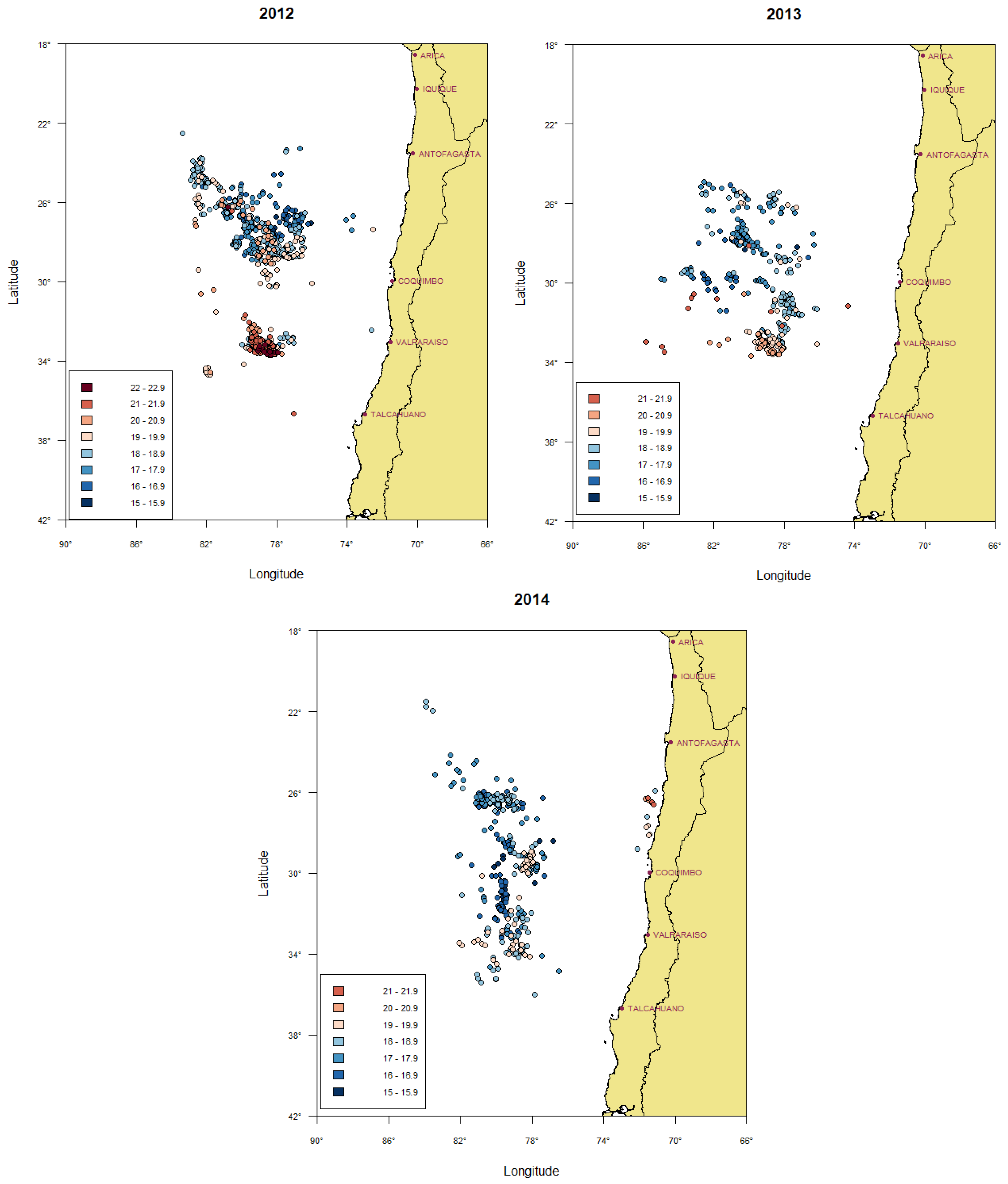
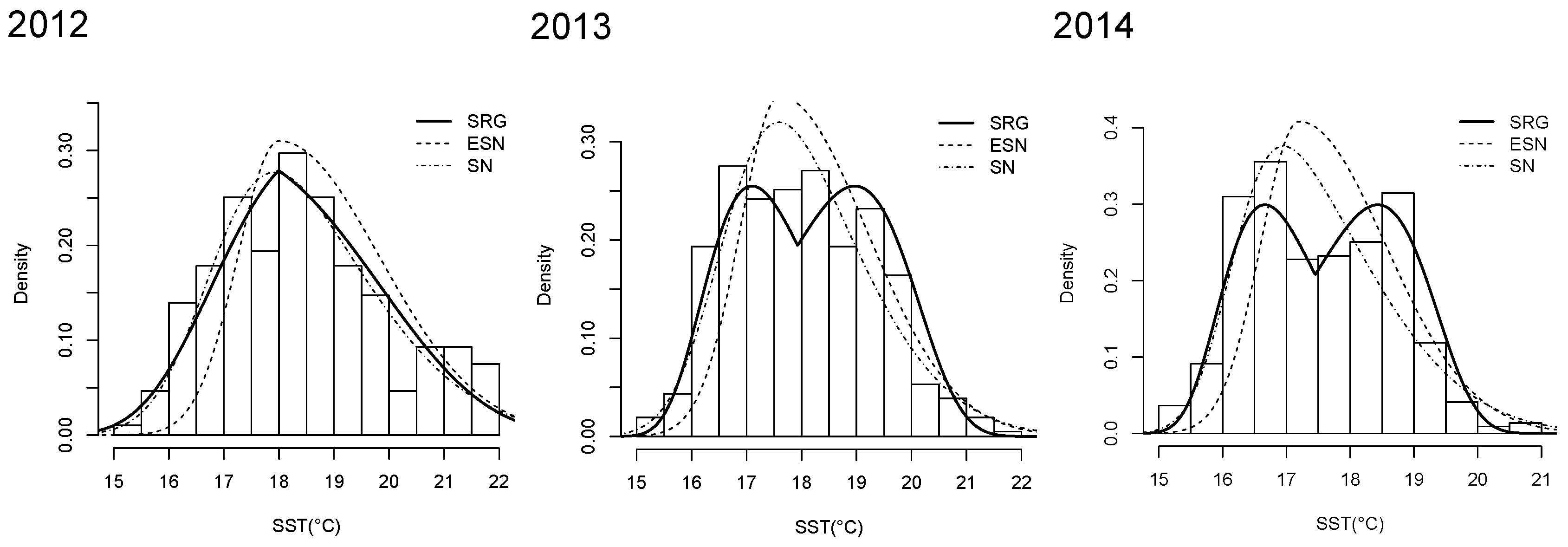
4.1. Sea Surface Temperature Data

The spatial information and SST data analyzed in this study were recorded by a scientific observer (whose labor concerns biological sampling of fishes, incidental captures of birds, turtles and marine mammals. Biological sampling was complemented with information such as time, longline and hook features, number of buoys, baits, etc.) (SO) in the Chilean longline fleet (industrial and artisanal), which was oriented to capture swordfish (Xiphias gladius, [23]) from 2012 to 2014 (obtaining a sampling of 83% in 2012, 55% in 2013, 90% in 2014, and 75% in 2012–2014). The covered area of the study was at ${21}^{°}$31′–${36}^{°}$39′ LS and ${71}^{°}$08′–${85}^{°}$52′ LW (see Figure 4).

SST records in swordfish captures are crucial for distributional analysis and fish abundance. Specifically, variations in SST are physical factors that control productivity, growth and migration of species [24]. In addition, SST is strongly correlated with atmospheric pressure at sea level and thus climatic time scales. Therefore, changes in SST overlap with ecosystem changes [25]. However, SST influence on ecosystems is not clear because other physical processes such as superficial warming, horizontal advection of currents, upwelling, etc. [11], modify SST. Therefore, SST anomalies could be symptomatic rather than causal.

4.1.1. SRG Parameter Estimates

Considering the smallest Akaike (AIC) and Schwarz (BIC) information criteria, we observed in

Table 1. Parameter estimates and their respective standard deviations (SD) for SST by year based on SRG, epsilon-skew-normal (ESN) and skew-normal (SN) models. For each model, log-likelihood function $\ell \left(\theta \right)$, $\theta =(\mu ,\sigma ,\eta ,\epsilon )$, Akaike’s (AIC) and Bayesian (BIC) information criteria, and goodness-of-fit tests (Kolmogorov–Smirnov (K–S), Anderson–Darling (A–D), and Cramer–von Mises, (C–V)) are also reported with respective p-values in parentheses.

Year	Model	Param.	Estim.	(S.D)	$\mathbf{\ell }\left(\theta \right)$	AIC	BIC	K–S	A–D	C–V
2012 ($n=774$)	SRG	$\mu$	17.992	0.103	−1401.896	2811.793	2830.399	0.044 (0.095)	2.014 (0.090)	0.214 (0.242)
		$\sigma$	2.590	0.067
		$\eta$	1.444	0.027
		$\epsilon$	−0.207	0.075
	ESN	$\theta$	18.000	0.031	−1507.534	3021.069	3035.023	0.118 (<0.01)	26.417 (<0.01)	2.059 (<0.01)
		$\varpi$	1.657	0.015
		$ϵ$	−0.418	0.069
	SN	$\xi$	16.777	0.114	−1404.581	2815.161	2829.116	0.041 (0.143)	1.752 (0.126)	0.198 (0.271)
		$\omega$	5.199	0.043
		$\lambda$	2.527	0.311
2013 ($n=415$)	SRG	$\mu$	17.935	0.061	−687.420	1382.839	1398.942	0.082 (0.010)	2.632 (0.042)	0.491 (0.041)
		$\sigma$	1.112	0.026
		$\eta$	0.432	0.021
		$\epsilon$	−0.108	0.029
	ESN	$\theta$	17.600	0.046	−716.375	1438.750	1450.827	0.089 (<0.01)	7.721 (<0.01)	0.970 (0.002)
		$\varpi$	1.328	0.026
		$ϵ$	−0.376	0.092
	SN	$\xi$	16.598	0.200	−691.531	1389.063	1401.140	0.066 (0.054)	2.002 (0.092)	0.328 (0.113)
		$\omega$	3.812	0.054
		$\lambda$	2.421	0.617
2014 ($n=439$)	SRG	$\mu$	17.454	0.048	−653.082	1314.164	1330.502	0.092 (<0.01)	2.848 (0.033)	0.533 (0.032)
		$\sigma$	0.896	0.020
		$\eta$	0.375	0.020
		$\epsilon$	−0.106	0.025
	ESN	$\theta$	17.200	0.053	−703.748	1413.496	1425.750	0.109 (<0.01)	11.996 (<0.01)	1.529 (<0.01)
		$\varpi$	0.956	0.035
		$ϵ$	−0.384	0.090
	SN	$\xi$	16.146	0.098	−666.984	1339.968	1352.222	0.096 (<0.01)	4.055 (<0.01)	0.711 (0.011)
		$\omega$	3.245	0.045
		$\lambda$	3.434	0.618

that SRG performs better than the SN and ESN models (see Appendix A and Appendix B, respectively). In addition, Table 1 shows the estimated parameters (based on the EM algorithm presented in Section 2) for SST datasets by year assuming SRG distribution. In 2012, a negative $\epsilon$ estimate corresponds to asymmetry to the right, and in 2013 and 2014 negative $\epsilon$ and $\eta$ close to zero produce a two-piece distribution to fit “cold” and “warm” temperatures (Figure 5).

To evaluate the goodness-of-fit test, the Kolmogorov–Smirnov (K–S), Anderson–Darling (A–D), and Cramer–von Mises (C–V) tests were considered for all models, commonly used to analyze the goodness-of-fit test of a particular distribution see, e.g., [26]). Considering a 95% confidence level, SRG fits perform well for 2012 and 2013, and on a 90% confidence level, the SRG fit performs well for 2014.

4.1.2. Information Quantifiers and Asymptotic Test

Parameters estimated from the SRG model and presented in Table 1 are used to perform the quantifiers of Section 3.1–Section 3.3 for SST in each year and for the asymptotic test of Section 3.4 for comparing SST between two years. The results of these analyses are shown in

Table 2. SRG Shannon, $H\left(Y\right)$, and Rényi, $R_{\alpha }\left(Y\right)$, $\alpha =2,3,4$, entropies for SST data. For each year, the KL divergence $K_0=\widehat{K}(Y_1,Y_2)$, statistic and its respective p-values of Equation (15) are reported. All reported $K_0$ estimates considered the estimated parameters and sample size n in Table 1.

Year	Quantifier	2012	2013	2014
	$H\left(Y\right)$	0.765	0.781	2.754
	$R_2\left(Y\right)$	0.384	−0.362	−0.365
	$R_3\left(Y\right)$	0.252	−0.417	−0.418
	$R_4\left(Y\right)$	0.163	−0.457	−0.457
2012	$K_0$	-	0.266	0.911
	Statistic	-	143.740	520.41
	p-value	-	<0.01	<0.01
2013	$K_0$	0.080	-	0.071
	Statistic	43.192	-	30.233
	p-value	<0.01	-	<0.01
2014	$K_0$	0.143	0.043	-
	Statistic	80.327	18.282	-
	p-value	<0.01	<0.01	-

. In Table 2, $K_0=\widehat{K}(Y_1,Y_2)$ represents the KL divergence between the years $Y_1$ (column) and $Y_2$ (row).

The first quantifiers (SE and RE) illustrate that the highest information of SST is obtained by SE and increases with the increment of years. For all RE, the highest information of SST is obtained in 2012 and is negative for 2013 and 2014 and similar during that period. Differences in information between SE and RE are produced by the independency of SE with parameter $\sigma$, while RE depends on three parameters as in Proposition 4.

In addition, the asymptotic test presented in Table 2 is analogous for all the years in both groups. In fact, the null hypothesis $H_0:{\mathbf{\theta }}_1={\mathbf{\theta }}_2$ is rejected at a 95% confidence level. This rejection is reinforced by high values of statistics $K_0$, produced by a high sample size of both groups ($n_1$ and $n_2$).

5. Conclusions

We have presented a methodology to compute the Shannon and the Rényi entropy and the Kullback–Leibler divergence for the family of Skew-Reflected-Gompertz distributions. Our methods consider the information quantifiers previously computed for the Gompertz distribution. Explicit formulas for Shannon and Rényi entropies (in terms of the Gompertz, Shannon and Rényi entropies, respectively), and the Kullback–Leibler divergence (using incomplete gamma function) facilitate easy computational implementation. Additionally, given the regularity conditions accomplished by the Skew-Reflected-Gompertz distribution, specifically by the Fisher information matrix convergence when $\epsilon$ is in $(-1,1)$, an asymptotic test for comparing two groups of datasets was developed.

The statistical application to South Pacific sea surface temperature was given. We first carried out SRG goodness-of-fit tests in samples over three years, where we find strong evidence (a 95% confidence level) for 2012, and moderate evidence (a 90% confidence level) for 2013 and 2014. The results show that the proposed methodology serves to compare two sets of samples, Skew-Reflected-Gompertz distributed. The proposed asymptotic test is therefore useful to detect anomalies in sea surface temperature, linked to extreme events influenced by environmental conditions [11,24,25]. We encourage researchers to consider the proposed methodology for further investigations related to environmental datasets [1].

References

1. Hoseinzadeh, A.; Maleki, M.; Khodadadi, Z.; Contreras-Reyes, J.E. The Skew-Reflected-Gompertz distribution for analyzing symmetric and asymmetric data. J. Comput. Appl. Math. 2019, 349, 132–141. [Google Scholar] [CrossRef]
2. Gompertz, B. On the nature of the function expressive of the law of human mortality, and on a new mode of determining the value of life contingencies. Philos. Trans. R. Soc. Lond. 1825, 115, 513–583. [Google Scholar] [CrossRef]
3. Arellano-Valle, R.B.; Contreras-Reyes, J.E.; Stehlík, M. Generalized skew-normal negentropy and its application to fish condition factor time series. Entropy 2017, 19, 528. [Google Scholar] [CrossRef]
4. Mudholkar, G.S.; Hutson, A.D. The epsilon-skew-normal distribution for analyzing near-normal data. J. Stat. Plan. Inference 2000, 83, 291–309. [Google Scholar] [CrossRef]
5. Maleki, M.; Mahmoudi, M.R. Two-Piece Location-Scale Distributions based on Scale Mixtures of Normal family. Commun. Stat. Theor. Meth. 2017, 46, 12356–12369. [Google Scholar] [CrossRef]
6. Moravveji, B.; Khodadai, Z.; Maleki, M. A Bayesian Analysis of Two-Piece distributions based on the Scale Mixtures of Normal Family. Iran. J. Sci. Technol. Trans. A 2019, 43, 991–1001. [Google Scholar] [CrossRef]
7. Contreras-Reyes, J.E. Rényi entropy and complexity measure for skew-gaussian distributions and related families. Physica A 2015, 433, 84–91. [Google Scholar] [CrossRef] [Green Version]
8. Contreras-Reyes, J.E. Analyzing fish condition factor index through skew-gaussian information theory quantifiers. Fluct. Noise Lett. 2016, 15, 1650013. [Google Scholar] [CrossRef]
9. Wang, Y.Q.; Derksen, R.W. The confirmation of the αβ model and the maximum entropy formulation in a thermal wake. Environmetrics 1998, 9, 269–282. [Google Scholar] [CrossRef]
10. De Queiroz, M.M.; Silva, R.W.; Loschi, R.H. Shannon entropy and Kullback–Leibler divergence in multivariate log fundamental skew-normal and related distributions. Can. J. Stat. 2016, 44, 219–237. [Google Scholar] [CrossRef]
11. Di Lorenzo, E.; Combes, V.; Keister, J.E.; Strub, P.T.; Thomas, A.C.; Franks, P.J.; Ohman, M.D.; Furtado, J.C.; Bracco, A.; Bograd, S.J.; et al. Synthesis of Pacific Ocean climate and ecosystem dynamics. Oceanography 2013, 26, 68–81. [Google Scholar] [CrossRef]
12. Salicrú, M.; Menéndez, M.L.; Pardo, L.; Morales, D. On the applications of divergence type measures in testing statistical hypothesis. J. Multivar. Anal. 1994, 51, 372–391. [Google Scholar] [CrossRef]
13. Maleki, M.; Contreras-Reyes, J.E.; Mahmoudi, M.R. Robust Mixture Modeling Based on Two-Piece Scale Mixtures of Normal Family. Axioms 2019, 8, 38. [Google Scholar] [CrossRef]
14. Arellano-Valle, R.B.; Gómez, H.W.; Quintana, F.A. Statistical inference for a general class of asymmetric distributions. J. Stat. Plan. Inference 2005, 128, 427–443. [Google Scholar] [CrossRef]
15. Jafari, A.A.; Tahmasebi, S.; Alizadeh, M. The beta-Gompertz distribution. Rev. Colomb. Estad. 2014, 37, 141–158. [Google Scholar] [CrossRef]
16. Shannon, C.E. A mathematical theory of communication. Bell Syst. Tech. J. 1948, 27, 379–423. [Google Scholar] [CrossRef]
17. Cover, T.M.; Thomas, J.A. Elements of Information Theory; Wiley & Son, Inc.: New York, NY, USA, 2006. [Google Scholar]
18. Rényi, A. Probability Theory; Dover Publications: New York, NY, USA, 2012. [Google Scholar]
19. Abu-Zinadah, H.H.; Aloufi, A.S. Some characterizations of the exponentiated Gompertz distribution. Int. Math. Forum 2014, 9, 1427–1439. [Google Scholar] [CrossRef] [Green Version]
20. Kullback, S.; Leibler, R.A. On information and sufficiency. Ann. Math. Stat. 1951, 22, 79–86. [Google Scholar] [CrossRef]
21. Bauckhage, C. Characterizations and Kullback–Leibler Divergence of Gompertz Distributions. arXiv 2014, arXiv:1402.3193. [Google Scholar]
22. R Core Team. A Language and Environment for Statistical Computing; R Foundation for Statistical Computing: Vienna, Austria, 2018; ISBN 3-900051-07-0. [Google Scholar]
23. Barría, P.; González, A.; Cortés, D.D.; Mora, S.; Miranda, H.; Cerna, F.; Cid, L.; Ortega, J.C. Seguimiento Pesquerías Recursos Altamente Migratorios, 2016. Convenio de Desempeño 2016; Informe Final, Subsecretaría de Economía y EMT; Instituto de Fomento Pesquero: Valparaíso, Chile, 2017. [Google Scholar]
24. Alheit, J.; Bernal, P. Effects of physical and biological changes on the biomass yield of the Humboldt Current ecosystem. In Large Marine Ecosystems—Stress, Mitigation and Sustainability; American Association for the Advancement of Science: Washington, DC, USA, 1993; pp. 53–68. [Google Scholar]
25. Oerder, V.; Bento, J.P.; Morales, C.E.; Hormazabal, S.; Pizarro, O. Coastal Upwelling Front Detection off Central Chile (36.5–37°S) and Spatio-Temporal Variability of Frontal Characteristics. Remote Sens. 2018, 10, 690. [Google Scholar] [CrossRef]
26. Lenart, A.; Missov, T.I. Goodness-of-fit tests for the Gompertz distribution. Commun. Stat. Theor. Meth. 2016, 45, 2920–2937. [Google Scholar] [CrossRef]
27. Bondon, P. Estimation of autoregressive models with epsilon-skew-normal innovations. J. Multivar. Anal. 2009, 100, 1761–1776. [Google Scholar] [CrossRef] [Green Version]
28. Azzalini, A. A Class of Distributions which includes the Normal Ones. Scand. J. Stat. 1985, 12, 171–178. [Google Scholar]
29. Henze, N. A probabilistic representation of the ‘skew-normal’ distribution. Scand. J. Stat. 1986, 13, 271–275. [Google Scholar]
Figure 1. Shannon entropy of Skew-Reflected-Gompertz (SRG) distributions for ε ( 1 , 1 ) and several values of η .
Mathematics 07 00403 g001
Figure 2. Rényi entropy of SRG distributions for σ = 1 , 1 < ε < 1 , several values of η and (a) α = 2 and (b) α = 5 values.
Mathematics 07 00403 g002
Figure 3. Plots of Kullback–Leibler (KL) divergence between Y 1 SRG ( 0 , σ 1 , η 1 , ε 1 ) and Y 2 SRG ( 0 , σ 2 , η 2 , ε 2 ) for values σ 1 = σ 2 = 1 and (a) η 1 = η 2 = 0.25 ; (b) η 1 = η 2 = 3 ; and (c) η 1 = η 2 = 10 .
Mathematics 07 00403 g003
Figure 4. Spatial distribution of Sea Surface Temperature (SST) observations by year ( 21 ° 31′– 36 ° 39′ LS, 71 ° 08′– 85 ° 52′ LW).
Mathematics 07 00403 g004
Figure 5. MLE fit of SRG, ESN and SN models for SST data by year.
Mathematics 07 00403 g005