Article

Predicting Maximal Gaps in Sets of Primes

by
Alexei Kourbatov
1,*,† and
Marek Wolf
2,*,†
1
JavaScripter.net, 15127 NE 24th St., #578, Redmond, WA 98052, USA
2
Faculty of Mathematics and Natural Sciences, Cardinal Stefan Wyszynski University, Wóycickiego 1/3, Bldg. 21, PL-01-938 Warsaw, Poland
*
Authors to whom correspondence should be addressed.
The authors contributed equally to this work.
Mathematics 2019, 7(5), 400; https://doi.org/10.3390/math7050400
Submission received: 5 April 2019 / Revised: 26 April 2019 / Accepted: 29 April 2019 / Published: 4 May 2019
(This article belongs to the Section Mathematics and Computer Science)

Abstract

:
Let q > r 1 be coprime integers. Let P c = P c ( q , r , H ) be an increasing sequence of primes p satisfying two conditions: (i) p r (mod q) and (ii) p starts a prime k-tuple with a given pattern H . Let π c ( x ) be the number of primes in P c not exceeding x. We heuristically derive formulas predicting the growth trend of the maximal gap G c ( x ) = max p x ( p p ) between successive primes p , p P c . Extensive computations for primes up to 10 14 show that a simple trend formula G c ( x ) x π c ( x ) · ( log π c ( x ) + O k ( 1 ) ) works well for maximal gaps between initial primes of k-tuples with k 2 (e.g., twin primes, prime triplets, etc.) in residue class r (mod q). For k = 1 , however, a more sophisticated formula G c ( x ) x π c ( x ) · log π c 2 ( x ) x + O ( log q ) gives a better prediction of maximal gap sizes. The latter includes the important special case of maximal gaps in the sequence of all primes ( k = 1 , q = 2 , r = 1 ). The distribution of appropriately rescaled maximal gaps G c ( x ) is close to the Gumbel extreme value distribution. Computations suggest that almost all maximal gaps satisfy a generalized strong form of Cramér’s conjecture. We also conjecture that the number of maximal gaps between primes in P c below x is O k ( log x ) .

1. Introduction

A prime gap is the difference between consecutive prime numbers. The sequence of prime gaps behaves quite erratically (see OEIS A001223 [1]). While the prime number theorem tells us that the average gap between primes near x is about log x , the actual gaps near x can be significantly larger or smaller than log x . We call a gap maximal if it is strictly greater than all gaps before it. Large gaps between primes have been studied by many authors; see, e.g., [2,3,4,5,6,7,8,9,10,11]. In the early 1910s, Ramanujan considered maximal prime gaps up to low 7-digit primes [2], p. 133. More than a century later, we know all maximal gaps between primes below 2 64 [3].
Let G ( x ) be the maximal gap between primes not exceeding x:
G ( x ) = max p n + 1 x ( p n + 1 p n ) .
Estimating G ( x ) is a subtle and delicate problem. Cramér [4] conjectured on probabilistic grounds that G ( x ) = O ( log 2 x ) , while Shanks [5] heuristically found that G ( x ) log 2 x . Granville [6] heuristically argued that for a certain subsequence of maximal gaps we should expect significantly larger sizes of G ( x ) ; namely, lim sup x G ( x ) log 2 x 2 e γ 1.1229 .
Baker, Harman, and Pintz [7] proved that G ( x ) = O ( x 0.525 ) ; indeed, computation suggests that G ( x ) < x 0.525 for x 127 . Ford, Green, Konyagin, Maynard, and Tao [8] proved that the order of G ( x ) is at least c log x log log x log log log log x log log log x , solving a long-standing conjecture of Erdős.
Earlier, we independently proposed formulas closely related to the Cramér and Shanks conjectures. Wolf [12,13,14] expressed the probable size of maximal gaps G ( x ) in terms of the prime-counting function  π ( x ) :
G ( x ) x π ( x ) · log π 2 ( x ) x + O ( 1 ) ,
which suggests an analog of Shanks conjecture G ( x ) log 2 x 2 log x log log x + O ( log x ) ; see also Cadwell [15]. Extending the problem statement to prime k-tuples, Kourbatov [16,17] empirically tested (for x 10 15 , k 7 ) the following heuristic formula for the probable size of maximal gaps G k ( x ) between prime k-tuples below x:
G k ( x ) a ( x ) · log x a ( x ) + O ( 1 ) ,
where a ( x ) is the expected average gap between the particular prime k-tuples near x. Similar to (1), Formula (2) also suggests an analog of the Shanks conjecture, G k ( x ) C log k + 1 x , with a negative correction term of size O k ( log x ) k log log x ; see also [18,19].
In this paper we study a further generalization of the prime gap growth problem, viz.: What happens to maximal gaps if we only look at primes in a specific residue class mod q? The new problem statement subsumes, as special cases, maximal prime gaps ( k = 1 , q = 2 ) as well as maximal gaps between prime k-tuples ( k 2 , q = 2 ). One of our present goals is to generalize Formulas (1) and (2) to gaps between primes in a residue class—and test them in computational experiments. Another goal is to investigate how many maximal gaps should be expected between primes p x in a residue class, with an additional (optional) condition that p starts a prime constellation of a certain type.

1.1. Notation

q, rcoprime integers, 1 r < q
p n the n-th prime;  { p n } = { 2 , 3 , 5 , 7 , 11 , }
P c = P c ( q , r , H ) increasing sequence of primes p such that (i) p r (mod q) and
(ii) p is the least prime in a prime k-tuple with a given pattern H .
Note: P c depends on q, r, k, and on the pattern H of the k-tuple.
When k = 1 , P c is the sequence of all primes p r (mod q).
H the k-tuple pattern of offsets: H = ( Δ 1 , Δ 2 , , Δ k ) (see Section 1.2)
gcd ( m , n ) the greatest common divisor of m and n
φ ( q ) Euler’s totient function (OEIS A000010)
φ k , H ( q ) Golubev’s generalization (5) of Euler’s totient (see Section 2.1.1)
Gumbel ( x ; α , μ ) the Gumbel distribution cdf: Gumbel ( x ; α , μ ) = e e x μ f α
Exp ( x ; α ) the exponential distribution cdf: Exp ( x ; α ) = 1 e x / α
α the scale parameter of exponential/Gumbel distributions, as applicable
μ the location parameter (mode) of the Gumbel distribution
γ the Euler–Mascheroni constant: γ = 0.57721
C k = C k , H the Hardy–Littlewood constants (see Appendix B)
log x the natural logarithm of x
li x the logarithmic integral of x: li x = 0 x d t log t = 2 x d t log t + 1.04516
Li k ( x ) the integral 2 x d t log k t (see Appendix C)
Gap measure functions:
G ( x ) the maximal gap between primes x
G q , r ( x ) the maximal gap between primes p = r + n q x (case k = 1 )
G c ( x ) the maximal gap between primes p P c not exceeding x
R c ( n ) the n-th record (maximal) gap between primes p P c
a, a c , a ¯ c the expected average gaps between primes in P c (see Section 2.2)
T, T c , T ¯ c trend functions predicting the growth of maximal gaps (see Section 2.3)
Gap counting functions: 1 1 1
N c ( x ) the number of maximal gaps G c with endpoints p x
N q , r ( x ) the number of maximal gaps G q , r with endpoints p x (case k = 1 )
τ q , r ( d , x ) the number of gaps of a given even size d = p p between successive
primes p , p r (mod q), with p x ; τ q , r ( d , x ) = 0 if q d or 2 d .
Prime counting functions: 1 1 1
π ( x ) the total number of primes p n x
π c ( x ) the total number of primes p P c not exceeding x
π ( x ; q , r ) the total number of primes p = r + n q x (case k = 1 )
Quantities with the c subscript may, in general, depend on q, r, k, and on the pattern of the prime k-tuple. However, average gaps a, a c , a ¯ c and trend functions T, T c , T ¯ c are independent of r. Expressions like π c 2 ( x ) or log 2 x denote the square of the respective function.

1.2. Definitions: Prime k-Tuples, Gaps, Sequence P c

Prime k-tuples are clusters of k consecutive primes that have an admissible pattern H . A k-tuple is admissible (infinitely repeatable) unless it is prohibited by an elementary divisibility argument. For example, the cluster of five numbers (p p + 2 , p + 4 , p + 6 , p + 8 ) is prohibited because one of the numbers is divisible by 5 (and, moreover, at least one of the numbers is divisible by 3); hence all these five numbers cannot simultaneously be prime infinitely often. Likewise, the cluster of three numbers (p p + 2 , p + 4 ) is prohibited because one of the numbers is divisible by 3; so these three numbers cannot simultaneously be prime infinitely often. In what follows, when we speak of a k-tuple, for certainty we will mean a densest admissible prime k-tuple, with a given k 7 . However, our observations can be extended to other admissible k-tuples, including those with larger k and not necessarily densest ones. The densest k-tuples that exist for a given k may sometimes be called prime constellations or prime k-tuplets. Below are examples of prime k-tuples with k = 2 , 4, 6.
  • Twin primes are pairs of consecutive primes that have the form (p, p + 2 ). This is the densest admissible pattern of two; H = ( 0 , 2 ) .
  • Prime quadruplets are clusters of four consecutive primes of the form (p, p + 2 , p + 6 , p + 8 ). This is the densest admissible pattern of four; H = ( 0 , 2 , 6 , 8 ) .
  • Prime sextuplets are clusters of six consecutive primes (p, p + 4 , p + 6 , p + 10 , p + 12 , p + 16 ). This is the densest admissible pattern of six; H = ( 0 , 4 , 6 , 10 , 12 , 16 ) .
A gap between prime k-tuples is the distance p p between the initial primes p and p in two consecutive k-tuples of the same type (i.e., with the same pattern). For example, the gap between twin prime pairs ( 17 , 19 ) and ( 29 , 31 ) is 12: p p = 29 17 = 12 .
A maximal gap between prime k-tuples is a gap that is strictly greater than all gaps between preceding k-tuples of the same type. For example, the gap of size 6 between twin primes ( 5 , 7 ) and ( 11 , 13 ) is maximal, while the gap (also of size 6) between twin primes ( 11 , 13 ) and ( 17 , 19 ) is not maximal.
Let q > r 1 be coprime integers. Let P c = P c ( q , r , H ) be an increasing sequence of primes p satisfying two conditions: (i) p r (mod q) and (ii) p starts a prime k-tuple with a given pattern H . Importantly, P c depends on q, r, k, and on the pattern of the k-tuple. When k = 1 , P c is the sequence of all primes p r (mod q). Gaps between primes in P c are defined as differences p p between successive primes p , p P c . As before, a gap is maximal if it is strictly greater than all preceding gaps. Accordingly, for successive primes p , p P c we define
G c ( x ) = max p < x p , p P c ( p p ) .
Studying maximal gaps between primes in P c is convenient. Indeed, if the modulus q used for defining P c is “not too small”, we get plenty of data to study maximal gaps; that is, we get many sequences of maximal gaps corresponding to P c ’s with different r for the same q, which allows us to study common properties of these sequences. (One such property is the average number of maximal gaps between primes in P c below x.) By contrast, data on maximal prime gaps are scarce: at present we know that there are only 80 maximal gaps between primes below 2 64 [3]. Even fewer maximal gaps are known between k-tuples of any given type [17].
Remark 1.
(i) 
In Section 2 we derive formulas predicting the most probable sizes of maximal gaps G c ( x ) . It is not known how close these most probable sizes might be to the maximal order of G c ( x ) . Thus, in the special case k = 1 , q = 2 , r = 1 , probable values of G ( x ) seem to be about log 2 x 2 log x log log x [13]; but it is not implausible that the maximal order of G ( x ) is closer to 2 e γ log 2 x [6]. For further discussion of extremely large gaps, see Section 3.5.
(ii) 
How hard is it to compute gaps in sequence P c ? Given k = 1 , q 10 3 and r coprime to q, our PARI/GP code (Appendix A) takes several hours to compute all maximal gaps in sequence P c up to 14-digit primes. In some numerical experiments, we carried out the computation all the way to 10 14 . In most cases, however, we stopped the computation at e 28 or at 10 12 or even earlier, to quickly gather statistics for all r coprime to q. A similar strategy was also used for sequences P c with k 2 (source code for k 2 is not included). See Section 3 for a detailed discussion of our numerical results.

1.3. Generalization to Other Subsets of Primes

Sequences P c include, as special cases, many different subsets of prime numbers: primes in a given residue class, twin primes, triplets, quadruplets, etc. However, formulas akin to (1) and (2) definitely have an even wider area of applicability. Namely, we expect that certain analogs of (1) or (2), possessing the general form
maximal gap size ( average gap near   x ) · L ( x ) , with L ( x ) c log x ,
will also be applicable to maximal gaps in the following subsets of primes:
  • the sequence of prime-indexed primes [20], A006450
  • higher iterates of prime-indexed primes [21,22,23], A038580
  • primes p = n 2 + 1 , n N [24], A002496
  • primes p = f ( n ) , where f ( n ) is an irreducible polynomial in n,
  • primes in sequences of Beatty type: p = β n + δ , n N , for a fixed irrational β > 1 and a fixed real δ [25], A132222.
The above list is by no means exhaustive, but it may serve as a starting point for future work.

1.4. When Are Equations (1), (2) Inapplicable?

Analogs of Equations (1) and (2) are not applicable to sequences where (almost) every gap is maximal. Examples of this kind include:
  • Mills primes [26], A051254,
  • base-B repunit primes [27], A076481,
  • primes nearest to e n (A037028),
  • in general, any sequence whose terms grow exponentially or super-exponentially.

2. Heuristics and Conjectures

We now focus on deriving analogs of Formulas (1) and (2) for sequences P c = P c ( q , r , H ) .

2.1. Equidistribution of k-Tuples

Everywhere we assume that q > r are coprime positive integers. Let π ( x ; q , r ) be the number of primes p r (mod q) such that p x . The prime number theorem for arithmetic progressions [28,29] establishes that
π ( x ; q , r ) li x φ ( q ) as   x .
Furthermore, the generalized Riemann hypothesis (GRH) implies that
π ( x ; q , r ) = li x φ ( q ) + O ε ( x 1 / 2 + ε ) for   any ε > 0 .
That is to say, the primes below x are approximately equally distributed among the φ ( q ) “allowed” residue classes (these classes form the reduced residue system modulo q). Roughly speaking, the GRH implies that, as x , the numbers π ( x ; q , r ) and li x / φ ( q ) almost agree in the left half of their digits.
Based on empirical evidence, below we conjecture that a similar phenomenon also occurs for prime k-tuples: in every H -allowed residue class (as defined below in Section 2.1.1) there are infinitely many primes starting an admissible k-tuple with a particular pattern H . Moreover, such primes are distributed approximately equally among all H -allowed residue classes modulo q. Our conjectures are closely related to the Hardy–Littlewood k-tuple conjecture [30] and the Bateman–Horn conjecture [31].

2.1.1. Counting the H -Allowed Residue Classes

Consider an example: take H = ( 0 , 2 ) . Which residue classes modulo 4 may contain the lesser prime p in a pair of twin primes ( p , p + 2 ) ? Clearly, the residue class 0 mod 4 is prohibited: all numbers in this class are even. The residue class 2 mod 4 is prohibited for the same reason. The remaining residue classes, p 1 mod 4 and p 3 mod 4, are not prohibited. We call these two classes H -allowed. Indeed, each of these two residue classes does contain lesser twin primes—and there are, conjecturally, infinitely many such primes in each class (see OEIS A071695 and A071698).
In general, given an admissible k-tuple with pattern H = ( Δ 1 , Δ 2 , , Δ k ) , we say that a residue class r (mod q) is H -allowed if
gcd ( r + Δ 1 , q ) = gcd ( r + Δ 2 , q ) = gcd ( r + Δ 3 , q ) = = gcd ( r + Δ k , q ) = 1 .
Thus a residue class is H -allowed if it is not prohibited (by divisibility considerations) from containing infinitely many primes p starting a prime k-tuple with pattern H .
How many residue classes modulo q are H -allowed? To count them, we will need an appropriate generalization of Euler’s totient φ ( q ) : Golubev’s totient functions [32,33,34]; see also [35], p. 289.
Definition 1.
Golubev’s totient φ k , H ( q ) is the number of H -allowed residue classes modulo q for a given pattern H = ( Δ 1 , , Δ k ) . More formally,
φ k , H ( q ) = 1 x q gcd ( x + Δ 1 , q ) = = gcd ( x + Δ k , q ) = 1 1 .
Example 1.
For prime quadruplets ( p , p + 2 , p + 6 , p + 8 ) we have
k = 4 , H = ( Δ 1 , Δ 2 , Δ 3 , Δ 4 ) = ( 0 , 2 , 6 , 8 ) , a n d φ 4 , H ( q ) = A 319516 ¯ ( q ) .
For instance, when q = 30 , we have φ 4 , H ( q ) = 1 : indeed, there is only one residue class, namely, p 11 (mod 30) where divisibility considerations allow infinitely many primes p at the beginning of prime quadruplets ( p , p + 2 , p + 6 , p + 8 ) .
Note that φ 1 ( q ) = φ ( q ) is Euler’s totient function, A000010; and, for densest admissible k-tuples, φ 2 , H ( q ) is A002472, see also Alder [36]; φ 3 , H ( q ) is A319534; φ 4 , H ( q ) is A319516; φ 5 , H ( q ) is A321029; and φ 6 , H ( q ) is A321030. Like Euler’s totient, the functions φ k , H are multiplicative [33].

2.1.2. The k-Tuple Infinitude Conjecture

We expect each of the H -allowed residue classes r (mod q) to contain infinitely many primes p starting admissible prime k-tuples with pattern H . In other words, the corresponding sequence P c = P c ( q , r , H ) is infinite.
Remark 2.
(i) 
The k-tuple infinitude conjecture generalizes Dirichlet’s theorem on arithmetic progressions [37].
(ii) 
The conjecture follows from the Bateman–Horn conjecture [31].

2.1.3. The k-Tuple Equidistribution Conjecture

We conjecture that the number of primes p P c , p x , is
π c ( x ) = C k , H φ k , H ( q ) Li k ( x ) + O η , H ( x η ) as   x ,
where η < 1 , the coefficient C k , H is the Hardy–Littlewood constant for the particular k-tuple (Appendix B), Li k ( x ) = 2 x log k t d t (Appendix C), and φ k , H ( q ) is Golubev’s totient function (5).
Remark 3.
(i) 
Conjecture (6) is akin to the GRH-based Equation (4); the latter pertains to the case k = 1 .
(ii) 
The conjecture is compatible with the Bateman–Horn and Hardy–Littlewood k-tuple conjectures but does not follow from them.
(iii) 
It is plausible that, similar to (4), in (6) we can take η = 1 2 + ε for any ε > 0 .

2.2. Average Gap Sizes

Consider a sequence P c = P c ( q , r , H ) , where the residue class r (mod q) is H -allowed. We define the expected average gaps between primes in P c as follows.
Definition 2.
Theexpected average gapbetween primes in P c belowx is
a c ( x ) = φ k , H ( q ) C k , H · x Li k ( x ) .
Definition 3.
Theexpected average gapbetween primes in P c nearx is
a ¯ c ( x ) = φ k , H ( q ) C k , H · log k x .
In view of the equidistribution conjecture (6), it is easy to see from these definitions that
x π c ( x ) a c ( x ) < a ¯ c ( x ) for large   x .
We have the limits (with very slow convergence):
lim x a c ( x ) a ¯ c ( x ) = 1 ,
lim x a ¯ c ( x ) a c ( x ) a ¯ c ( x ) · log x = k .

2.3. Maximal Gap Sizes

Recall that Formula (1) is applicable to the special case q = 2 , k = 1 [12,13,14], while (2) is applicable to the special cases q = 2 , k 2 [16]. We are now ready to generalize (1) and (2) for predicting maximal gaps between primes in sequences P c with q 2 .

2.3.1. Case of k-Tuples: k 2

Consider a probabilistic example. Suppose that intervals between rare random events are exponentially distributed, with cdf Exp ( ξ ; α ) = 1 e ξ / α , where α is the mean interval between events. If our observations of the events continue for x seconds, extreme value theory (EVT) predicts that the expected maximal interval between events is
expected maximal interval = α log x α + O ( α ) = x Π ( x ) log Π ( x ) + O ( α ) ,
where Π ( x ) x / α is the total count of the events we observed in x seconds. (For details on deriving Equation (11), see e.g., [38], pp. 114–116 or [16], Section 8.)
By analogy with EVT, we define the expected trend functions for maximal gaps as follows.
Definition 4.
Thelower trendof maximal gaps between primes in P c is
T c ( x ) = a c ( x ) · log C k , H Li k ( x ) φ k , H ( q ) .
In view of the equidistribution conjecture (6),
T c ( x ) a c ( x ) · log π c ( x ) x π c ( x ) · log π c ( x ) as   x .
We also define another trend function, T ¯ c ( x ) , which is simpler because it does not use Li k ( x ) .
Definition 5.
Theupper trendof maximal gaps between primes in P c is
T ¯ c ( x ) = a ¯ c ( x ) · log x a ¯ c ( x ) .
The above definitions imply that
T c ( x ) < T ¯ c ( x ) < C k , H 1 φ k , H ( q ) · log k + 1 x for large   x .
At the same time, we have the asymptotic equivalence:
T c ( x ) T ¯ c ( x ) C k , H 1 φ k , H ( q ) · log k + 1 x as   x .
We have the limits (convergence is quite slow):
lim x T ¯ c ( x ) T c ( x ) a ¯ c ( x ) = k ,
lim x C k , H 1 φ k , H ( q ) log k + 1 p T ¯ c ( x ) a ¯ c ( x ) log log x = k .
Therefore, T ¯ c ( x ) T c ( x ) = O k ( a ¯ c ) , while C k , H 1 φ k , H ( q ) log k + 1 p T ¯ c ( x ) = O k ( a ¯ c log log x ) .
We make the following conjectures regarding the behavior of maximal gaps G c ( x ) .
Conjecture on the trend of G c ( x ) . For any sequence P c with k 2 , a positive proportion of maximal gaps G c ( x ) satisfy the double inequality
T c ( x ) G c ( x ) T ¯ c ( x ) as   x ,
and the difference G c ( x ) T ¯ c ( x ) changes its sign infinitely often.
Generalized Cramér conjecture for G c ( p ) . Almost all maximal gaps G c ( p ) satisfy
G c ( p ) < C k , H 1 φ k , H ( q ) log k + 1 p .
Generalized Shanks conjecture for G c ( p ) . Almost all maximal gaps G c ( p ) satisfy
G c ( p ) C k , H 1 φ k , H ( q ) log k + 1 p as   p .
Here G c ( p ) denotes the maximal gap that ends at the prime p.

2.3.2. Case of Primes: k = 1

The EVT-based trend Formulas (12) and (14) work well for maximal gaps between k-tuples, k 2 . However, when k = 1 , the observed sizes of maximal gaps G q , r ( x ) between primes in residue class r mod q are usually a little less than predicted by the corresponding lower trend formula akin to (12). For example, with k = 1 and q = 2 , the most probable values of maximal prime gaps G ( x ) turn out to be less than the EVT-predicted value x log li x li x —less by approximately log x log log x (cf. Cadwell [15]), p. 912. In this respect, primes do not behave like “random darts”. Instead, the situation looks as if primes “conspire together” so that each prime p n x lowers the typical maximal gap G ( x ) by about p n 1 log x ; indeed, we have p n x p n 1 log log x . Below we offer a heuristic explanation of this phenomenon.
Let τ q , r ( d , x ) be the number of gaps of a given even size d = p p between successive primes p , p r (mod q), p x . Empirically, the function τ q , r has the form (cf. [13,39,40])
τ q , r ( d , x ) P q ( d ) B q ( x ) e d · A q ( x ) ,
where P q ( d ) is an oscillating factor (encoding a form of singular series), and
τ q , r ( d , x ) = P q ( d ) = 0 if q d or 2 d .
The essential point now is that we can find the unknown functions A q ( x ) and B q ( x ) in (22) just by assuming the exponential decay of τ q , r as a function of d and employing the following two conditions (which are true by definition of τ q , r ):
( a ) the total number of gaps is d = 2 G q , r ( x ) τ q , r ( d , x ) π ( x ; q , r ) ;
( b ) the total length of gaps is d = 2 G q , r ( x ) d · τ q , r ( d , x ) x .
The erratic behavior of the oscillating factor P q ( d ) presents an obstacle in the calculation of sums (24) and (25). We will assume that, for sufficiently regular functions f ( d , x ) ,
d P q ( d ) f ( d , x ) s d f ( d , x ) ,
where s is such that, on average, P q ( d ) s ; and the summation is for d such that both sides of (26) are non-zero. Extending the summation in Equations  (24), (25) to infinity, using (26), and writing
d = c j , j N , c = LCM ( 2 , q ) = O ( q ) , s = lim n 1 n j = 1 n P q ( c j ) ,
we obtain two series expressions: (24) gives us a geometric series
d = 2 τ q , r ( d , x ) s B q ( x ) j = 1 e c j A q ( x ) = s B q ( x ) · e c A q ( x ) 1 e c A q ( x ) π ( x ; q , r ) ,
while (25) yields a differentiated geometric series
d = 2 d · τ q , r ( d , x ) c s B q ( x ) j = 1 j e c j A q ( x ) = c s B q ( x ) · e c A q ( x ) ( 1 e c A q ( x ) ) 2 x .
Thus we have obtained two equations:
s B q ( x ) · e c A q ( x ) 1 e c A q ( x ) π ( x ; q , r ) , c s B q ( x ) · e c A q ( x ) ( 1 e c A q ( x ) ) 2 x .
To solve these equations, we use the approximations e c A q ( x ) 1 and 1 e c A q ( x ) c A q ( x ) (which is justified because we expect A q ( x ) 0 for large x). In this way we obtain
A q ( x ) π ( x ; q , r ) x , B q ( x ) c π 2 ( x ; q , r ) s x .
A posteriori we indeed see that A q ( x ) 0 as x . Substituting (29) into (22) we get
τ q , r ( d , x ) P q ( d ) c π 2 ( x ; q , r ) s x e d · π ( x ; q , r ) / x .
From (30) we can obtain an approximate formula for G q , r ( x ) . Note that τ q , r ( d , x ) = 1 when the gap of size d is maximal—in which case we have d = G q , r ( x ) . So, to get an approximate value of the maximal gap G q , r ( x ) , we solve for d the equation τ q , r ( d , x ) = 1 , or
c π 2 ( x ; q , r ) x e d · π ( x ; q , r ) / x 1 ,
where we skipped P q ( d ) / s because, on average, P q ( d ) s . Taking the log of both sides of (31) we find the solution G q , r ( x ) expressed directly in terms of π ( x ; q , r ) :
G q , r ( x ) x π ( x ; q , r ) · log π 2 ( x ; q , r ) x + log c .
Since π ( x ; q , r ) li x φ ( q ) and log π 2 ( x ; q , r ) x 2 log li x φ ( q ) log x , we can state the following
Conjecture on the trend of G q , r ( x ) . The most probable sizes of maximal gaps G q , r ( x ) are near a trend curve T ( q , x ) :
G q , r ( x ) T ( q , x ) = φ ( q ) x li x · 2 log li x φ ( q ) log x + b ,
where b = b ( q , x ) = O ( log q ) tends to a constant as x . The difference G q , r ( x ) T ( q , x ) changes its sign infinitely often.
Further, we expect that the width of distribution of the maximal gaps near x is O q ( log x ) ; i.e., the width of distribution is on the order of the average gap φ ( q ) log x (see Section 3.2). On the other hand, for large x, the trend (33) differs from the line φ ( q ) log 2 x by O q ( log x log log x ) , that is, by much more than the average gap. This suggests natural generalizations of the Cramér and Shanks conjectures:
Generalized Cramér conjecture for G q , r ( p ) . Almost all maximal gaps G q , r ( p ) satisfy
G q , r ( p ) < φ ( q ) log 2 p .
Generalized Shanks conjecture for G q , r ( p ) . Almost all maximal gaps G q , r ( p ) satisfy
G q , r ( p ) φ ( q ) log 2 p as   p .
Conjectures (34) and (35) can be viewed as particular cases of (20), (21) for k = 1 .

2.4. How Many Maximal Gaps Are There?

This section generalizes the heuristic reasoning of [41], Section 2.3. Let R c ( n ) be the size of the n-th record (maximal) gap between primes in P c . Denote by N c ( x ) the total number of maximal gaps observed between primes in P c not exceeding x. Let = ( x ; q , H ) be a continuous slowly varying function estimating mean r ( N c ( e x ) N c ( x ) ) , the average number of maximal gaps between primes in P c , with the upper endpoints p [ x , e x ] . For x , we will heuristically argue that if the limit of exists, then the limit is k + 1 . Suppose that
lim x N c ( x ) log x = lim x mean r N c ( x ) log x = lim x ( x ; q , H ) = * > 0 ,
and the limit * is independent of q. Let n be a “typical” number of maximal gaps up to x; our assumption lim x = * means that
n * log x as   x .
For large n, we can estimate the order of magnitude of the typical n-th maximal gap R c ( n ) using the generalized Cramér and Shanks conjectures (20) and (21):
R c ( n ) = G c ( x ) C k , H 1 φ k , H ( q ) log k + 1 x C k , H 1 φ k , H ( q ) n k + 1 * k + 1 .
Define Δ R c ( n ) = R c ( n + 1 ) R c ( n ) . By Formula (37), for large q and large n we have
mean r R c ( n ) C k , H 1 φ k , H ( q ) n k + 1 * k + 1 ,
mean r Δ R c ( n ) = mean r R c ( n + 1 ) R c ( n ) C k , H 1 φ k , H ( q ) * k + 1 · ( n + 1 ) k + 1 n k + 1 C k , H 1 φ k , H ( q ) * k + 1 · ( k + 1 ) n k ,
where the mean is taken over all H -allowed residue classes; see Section 2.1.1. Combining this with (36), we find
mean r Δ R c ( n ) k + 1 * · C k , H 1 φ k , H ( q ) log k x .
On the other hand, heuristically we expect that, on average, two consecutive record gaps should differ by the “local” average gap (8) between primes in P c :
mean r Δ R c ( n ) C k , H 1 φ k , H ( q ) log k x ( average gap near x ) .
Together, Equations (38) and (39) imply that
* = k + 1 .
Therefore, for large x we should expect (see Section 3.3 and Section 3.4; cf. [42])
N c ( x ) ( k + 1 ) log x as   x .
Special cases. For the number N q , r of maximal gaps between primes p r (mod q) we have
N q , r ( x ) 2 log x as   x .
This is asymptotically equivalent to the following semi-empirical formula for the number of maximal prime gaps up to x (i.e., for the special case k = 1 , q = 2 ; see [43], Section 3.4; OEIS A005669):
N 2 , 1 ( x ) 2 log li x as   x .
Formula (42) tells us that maximal prime gaps occur, on average, about twice as often as records in an i.i.d. random sequence of li x terms. Note also the following straightforward generalization of (42) giving a very rough estimate of N q , r ( x ) in the general case:
N q , r ( x ) max 0 , 2 log li x φ ( q ) .
Computation shows that, for the special case of maximal prime gaps G ( x ) , Formula (42) works quite well. However, the more general Formula (43) usually overestimates N q , r ( x ) . At the same time, the right-hand side of (43) is less than 2 log x . Thus the right-hand sides of (41) as well as (43) overestimate the actual gap counts N q , r ( x ) in most cases.
In Section 3.3 we will see an alternative (a posteriori) approximation based on the average number of maximal gaps observed for primes in the interval [ x , e x ] . Namely, the estimated average number ( x ; q , H ) of maximal gaps with endpoints in [ x , e x ] is
( x ; q , H ) mean r ( N c ( e x ) N c ( x ) ) k + 1 κ ( q , H ) log x + δ ( q , H ) .

3. Numerical Results

To test our conjectures of the previous section, we performed extensive computational experiments. We used PARI/GP (see Appendix A for code examples) to compute maximal gaps G c between initial primes p = r + n q P c in densest admissible prime k-tuples, k 6 . We experimented with many different values of q [ 4 , 10 5 ] . To assemble a complete data set of maximal gaps for a given q, we used all H -allowed residue classes r (mod q). For additional details of our computational experiments with maximal gaps between primes p = r + n q (i.e., for the case k = 1 ), see also [43], Section 3. In this section we omit the subscript H in φ k and C k because we are working with densest k-tuples: for each k = 2 , 4 , 6 there is only one densest pattern H , while for each k = 3 , 5 , 7 there are two densest patterns H , with equal numerical values of functions φ k ( q ) and equal Hardy–Littlewood constants C k .

3.1. The Growth Trend of Maximal Gaps
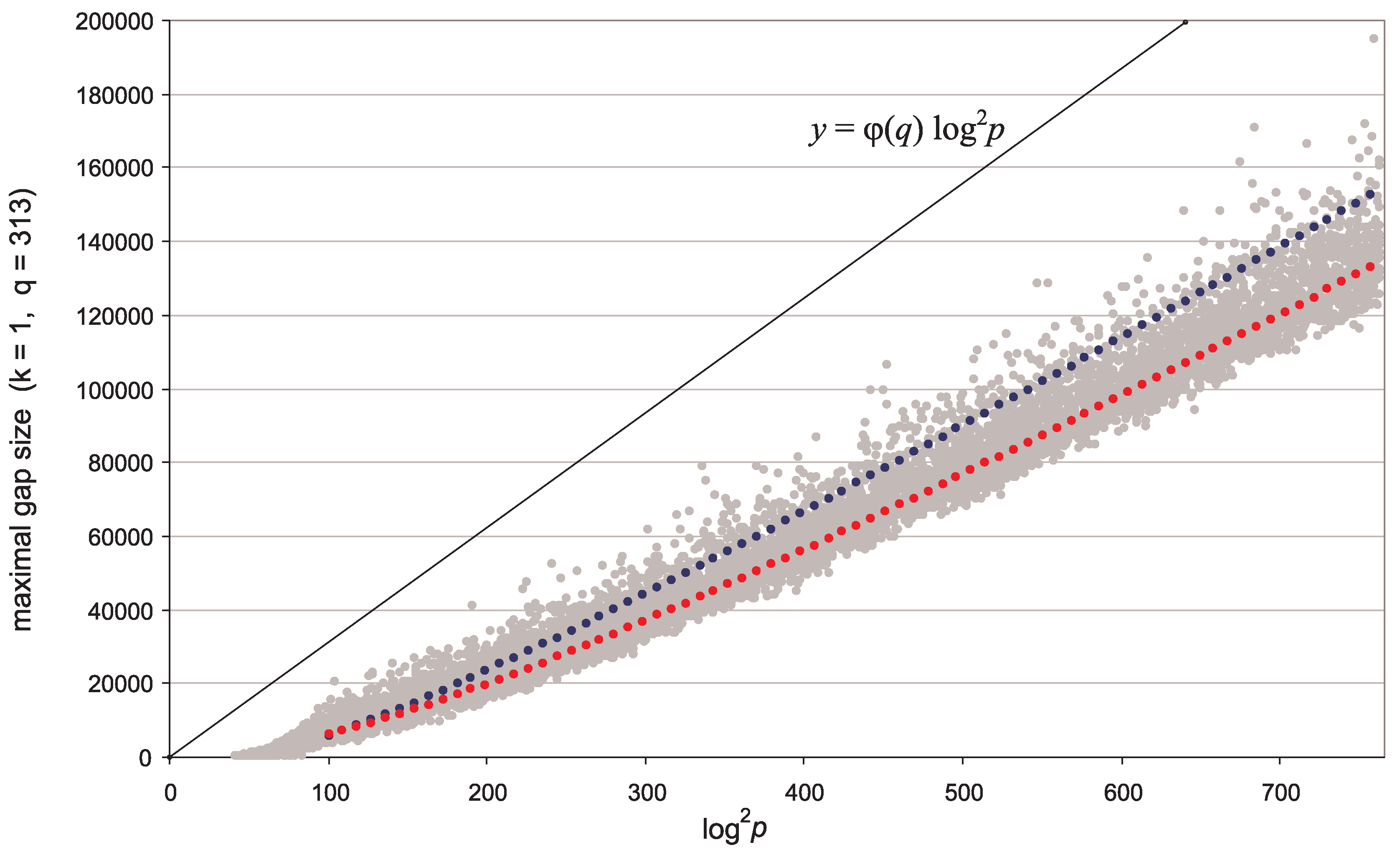
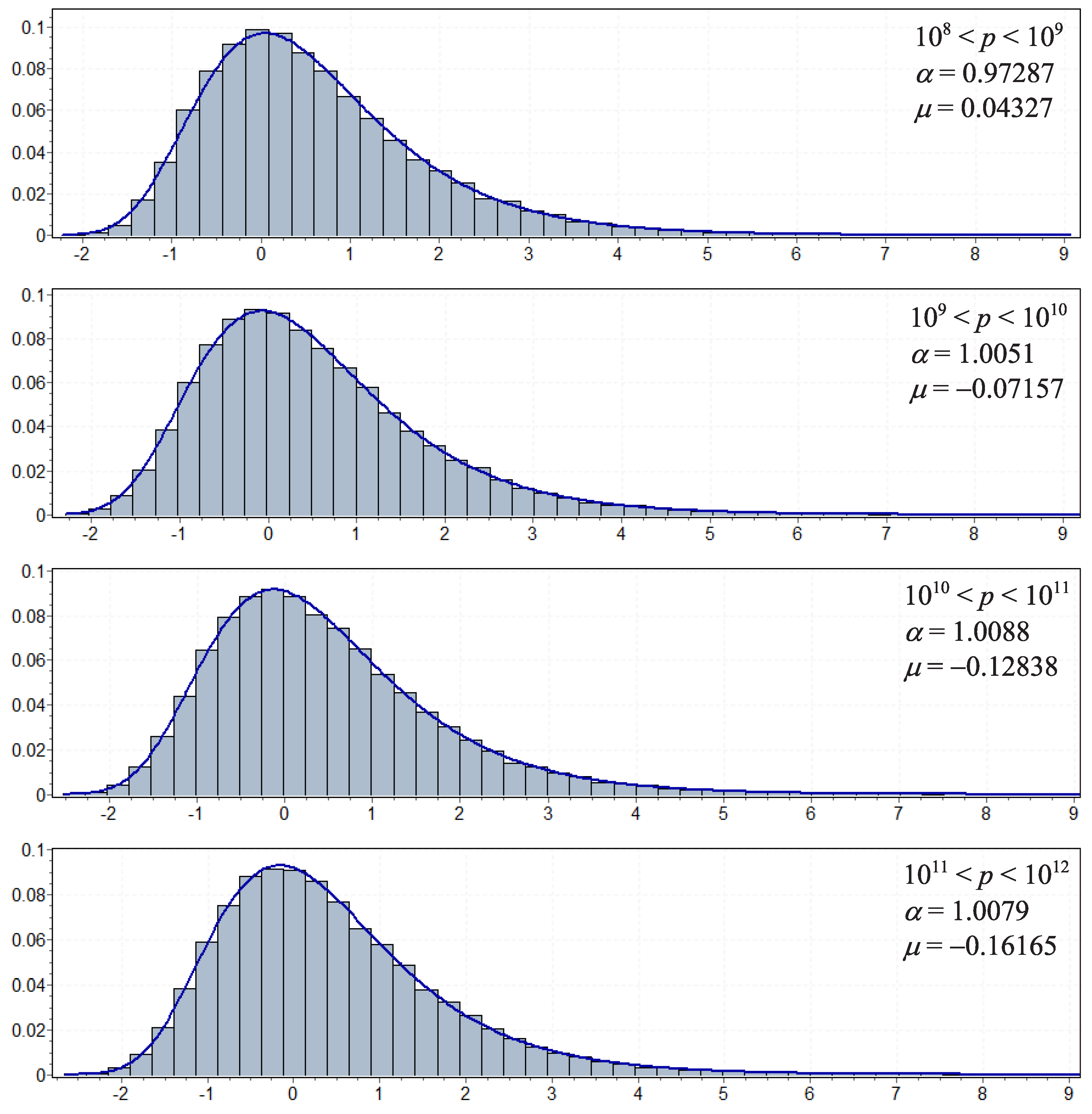
The vast majority of maximal gap sizes G c ( x ) are indeed observed near the trend curves predicted in Section 2.3. Specifically, for maximal gaps G c between primes p = r + n q P c in k-tuples ( k 2 ), the gap sizes are mostly found in the neighborhood of the corresponding trend curves of Equations (12) and (14) derived from extreme value theory. However, for k = 1 , the trend Equation (33) gives a better prediction of maximal gaps G q , r .
Figure 1, Figure 2 and Figure 3 illustrate our numerical results for k = 1 , 2 , 6 , q = 313 . The horizontal axis in these figures is log k + 1 p for end-of-gap primes p. Note that all gaps shown in the figures satisfy the generalized Cramér conjecture, i.e., inequalities (20), (34); for rare exceptions, see Section 3.5. Results for other values of q look similar to Figure 1, Figure 2 and Figure 3.
Numerical evidence suggests that
  • For k = 1 (the case of maximal gaps G q , r between primes p = r + n q ) the EVT-based trend curve φ ( q ) x li x log li x φ ( q ) goes too high (Figure 1, blue curve). Meanwhile, the trend (33) (Figure 1, red curve)
    T ( q , x ) = φ ( q ) x li x · 2 log li x φ ( q ) log x + b
    satisfactorily predicts gap sizes G q , r ( x ) , with the empirical correction term
    b = b ( q , x ) b 0 + b 1 ( log log x ) b 2 log φ ( q ) log φ ( q ) ,
    where the parameter values
    b 0 = 1 , b 1 = 4 , b 2 = 2.7
    are close to optimal for q [ 10 2 , 10 5 ] and x [ 10 7 , 10 14 ] . Here the qualifier optimal is to be understood in conjunction with the rescaling transformation (47) introduced below in Section 3.2. A trend T ( q , x ) is optimal if after transformation (47) the most probable rescaled values w turn out to be near zero, and the mode of best-fit Gumbel distribution for w-values is also close to zero, μ 0 ; see Figure 4. In view of (45) it is possible that, for all q, the optimal term b in (33) has the form b ( q , x ) = ( 1 + β ( q , x ) ) · log φ ( q ) log φ ( q ) , where β ( q , x ) very slowly decreases to zero as x . (Note that in Section 2.3.2 we correctly estimated b to be O ( log q ) but did not predict the appearance of Euler’s function φ ( q ) in the term b.)
  • For k = 2 , approximately half of maximal gaps G c between lesser twin primes p P c are below the lower trend curve T c ( x ) of Equation (12), while the other half are above that curve; see Figure 2.
  • For k 3 , more than half of maximal gaps G c are usually above the lower trend curve T c ( x ) of Equation (12). At the same time, more than half of maximal gaps are usually below the upper trend curve T ¯ c ( x ) of Equation (14); see Figure 3. Recall that the two trend curves T c and T ¯ c are within k a ¯ c from each other as x ; see (17).
As noted by Brent [44], twin primes seem to be more random than primes. We can add that, likewise, maximal gaps G q , r between primes in a residue class seem to be somewhat less random than those for prime k-tuples; primes p r (mod q) do not go quite as far from each other as we would expect based on extreme value theory. Pintz [45] discusses various other aspects of the “random” and not-so-random behavior of primes.

3.2. The Distribution of Maximal Gaps

In Section 3.1 we have tested equations that determine the growth trend of maximal gaps between primes in sequences P c . How are maximal gap sizes distributed in the neighborhood of their respective trend?
We will perform a rescaling transformation (motivated by extreme value theory): subtract the trend from the actual gap size, and then divide the result by a natural unit, the “local” average gap. This way each maximal gap size is mapped to its rescaled value:
maximal gap size   G rescaled value = G trend average gap .
Gaps above the trend curve are mapped to positive rescaled values, while gaps below the trend curve are mapped to negative rescaled values.
Case k = 1 . For maximal gaps G q , r between primes p r (mod q), the trend function T is given by Equations (33), (45) and (46). The rescaling operation has the form
G q , r ( x ) w = G q , r ( x ) T ( q , x ) a ( q , x ) .
where a ( q , x ) = φ ( q ) x li x . Figure 4 shows histograms of rescaled values w for maximal gaps G q , r between primes p r (mod q) for q = 16001 .
Case k 2 . For maximal gaps G c between prime k-tuples with p = r + n q P c , we can use the trend T c of Equation (12). Then the rescaling operation has the form
G c ( x ) h = G c ( x ) T c ( x ) a c ( x ) ,
where a c ( x ) is defined by (7). Figure 5 shows histograms of rescaled values h for maximal gaps G c between lesser twin primes p = r + n q P c for q = 16001, k = 2 .
In both Figure 4 and Figure 5, note that the histograms and fitting distributions are skewed to the right, i.e., the right tail is longer and heavier. Among two-parameter distributions, the Gumbel extreme value distribution is a very good fit; cf. [46,47]. This was true in all our computational experiments.
Remark 4.
For all histograms shown in Figure 4 and Figure 5, the Kolmogorov–Smirnov goodness-of-fit statistic is less than 0.01; in fact, for most of the histograms, the goodness-of-fit statistic is about 0.003.
If we look at three-parameter distributions, then an excellent fit is the Generalized Extreme Value (GEV) distribution, which includes the Gumbel distribution as a special case. The shape parameter in the best-fit GEV distributions is close to zero; note that the Gumbel distribution is a GEV distribution whose shape parameter is exactly zero. So could the Gumbel distribution be the limit law for appropriately rescaled sequences of maximal gaps G q , r ( p ) and G c ( p ) as p ? Does such a limiting distribution exist at all?
The scale parameter α . For k = 1 , we observed that the scale parameter of best-fit Gumbel distributions for w-values (47) was in the range α [ 0.7 , 1 ] . The parameter α seems to slowly grow towards 1 as p ; see Figure 4. For k 2 , the scale parameter of best-fit Gumbel distributions for h-values (48) was usually a little over 1; see Figure 5. However, if instead of (48) we use the (simpler) rescaling transformation
G c ( x ) h ¯ = G c ( x ) T ¯ c ( x ) a ¯ c ( x ) ,
where a ¯ c and T ¯ c are defined, respectively, by (8) and (14), then the resulting Gumbel distributions of h ¯ -values will typically have scales α a little below 1. In a similar experiment with random gaps, the scale was also close to 1; see [43], Section 3.3.

3.3. Counting the Maximal Gaps

We used PARI/GP function findallgaps (see source code in Appendix A.2) to determine average numbers of maximal gaps G q , r between primes p = r + n q , p [ x , e x ] , for x = e j , j = 1 , 2 , , 27 . Similar statistics were also gathered for gaps G c . Figure 6, Figure 7, Figure 8 and Figure 9 show the results of this computation for q = 16001 , k 4 . When x is large, the average number of maximal gaps G c for p [ x , e x ] indeed seems to very slowly approach k + 1 , as predicted by Equation (40). When x is small ( x < q / e ), there is at most one prime p [ 2 , e x ] in sequence P c —and often there are no such primes at all; accordingly, we see no gaps ending in [ x , e x ] , and the corresponding plot points in Figure 6, Figure 7, Figure 8 and Figure 9 are zero.
Starting from some x 0 > q / e , the gap counts in [ x , e x ] are no longer zero. Here we observe a “transition region” in which the mean number of maximal gaps G c ( p ) for primes p [ x , e x ] grows from 0 to a little over 1, while x increases by about 3 orders of magnitude from x 0 . The non-monotonic behavior of plot points in the transition region is explained, in part, by the fact that here the gap size may be comparable to the size of intervals [ x , e x ] . Then, for larger x, the typical number of gaps G c between k-tuples continues to slowly increase; specifically, the graph of mean ( N c ( e x ) N c ( x ) ) vs.  log x is closely approximated by a hyperbola with horizontal asymptote y = k + 1 ; see Equation (40) in Section 2.4. Why do the observed curves resemble hyperbolas? If we were working with random gaps, then perhaps the curves could be explained using the theory of records; cf. [42]. But primes are not random numbers; and so we simply have to treat the hyperbolas in Figure 6, Figure 7, Figure 8 and Figure 9 as an experimental fact.

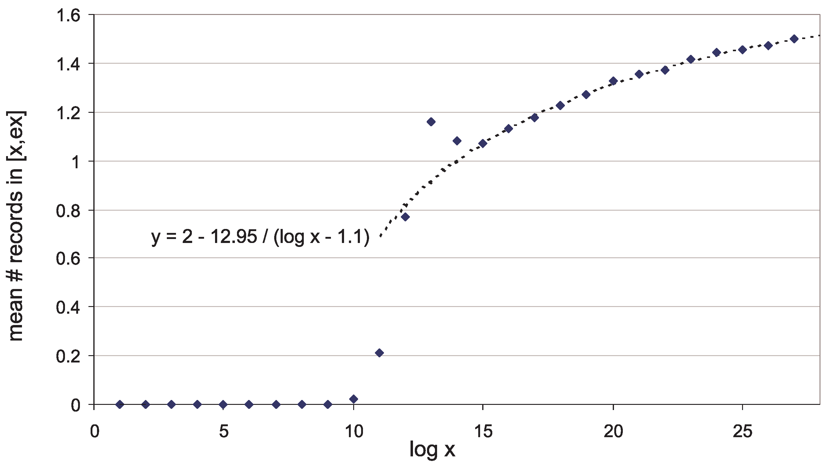
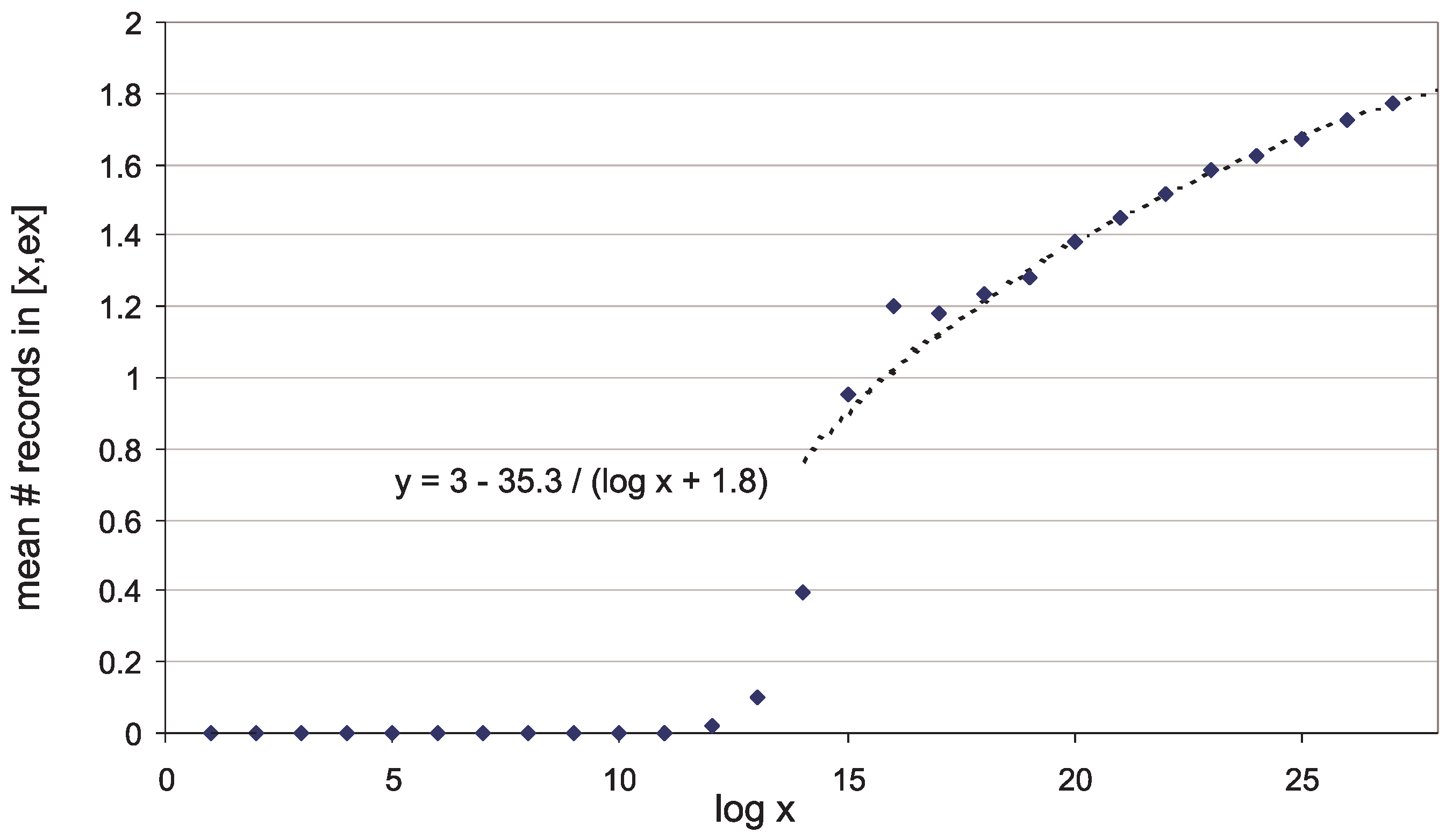
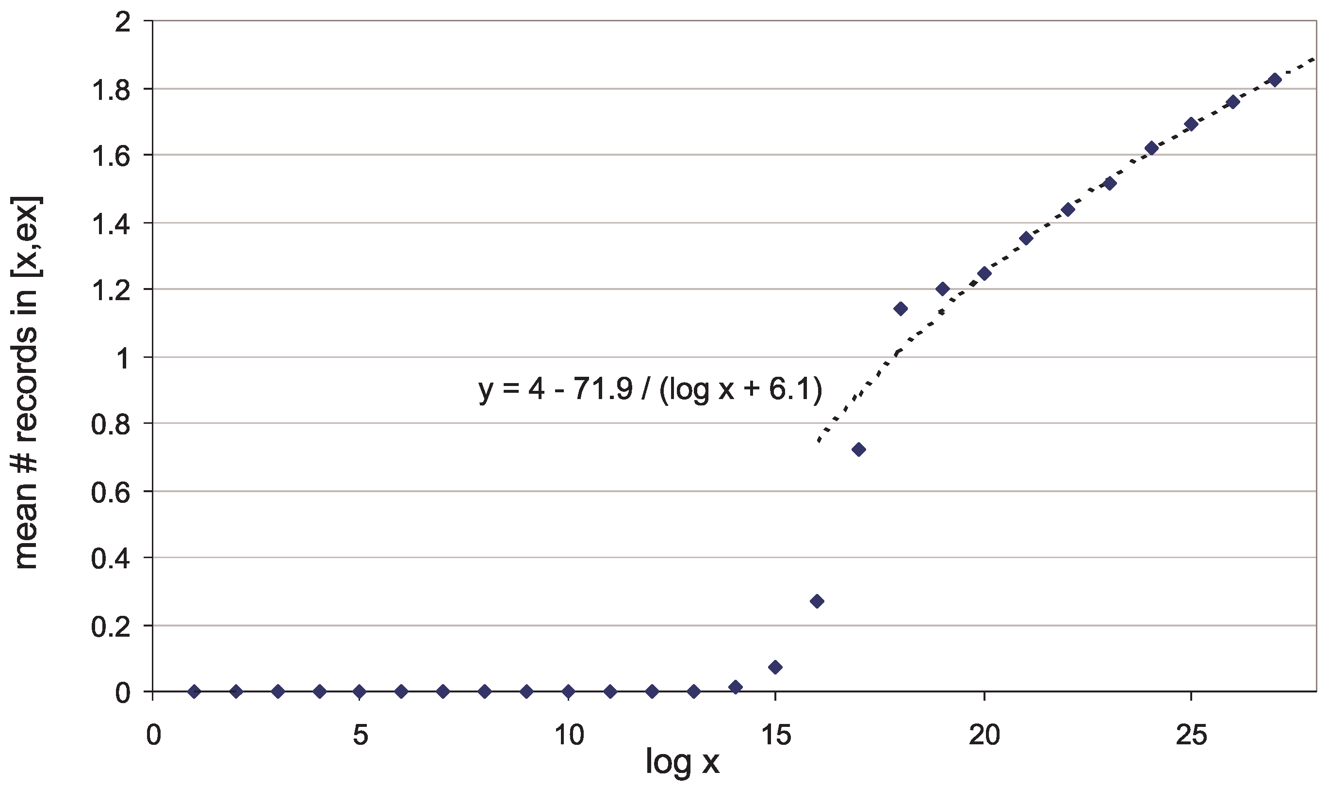
3.4. How Long Do We Wait for the Next Maximal Gap?

Let P(n) = A002386(n) and P’(n) = A000101(n) be the lower and upper endpoints of the n-th record (maximal) gap R ( n ) between primes: R(n) = A005250(n) = P’(n) − P(n).
Consider the distances P ( n ) P ( n 1 ) from one maximal gap to the next. (In statistics, a similar quantity is sometimes called “inter-record times”). In Figure 10 we present a plot of these distances; the figure also shows the corresponding plot for twin primes. As can be seen from Figure 10, the quantity P ( n ) P ( n 1 ) grows approximately exponentially with n (but not monotonically). Indeed, typical inter-record times are expected to satisfy
log ( P ( n ) P ( n 1 ) ) < log P ( n ) n 2 as   n .
The asymptotic equivalence ∼ in Equations (50) and (51) is a restatement of Equations (40) and (41). It would be logically unsound to suppose that log ( P ( n ) P ( n 1 ) ) ? log P ( n ) because we cannot exclude the possibility that log ( P ( n ) P ( n 1 ) ) might (very rarely) become as small as log G ( x ) 2 log log x , where x = P ( n ) .
More generally, let P c ( n ) and P c ( n ) be the endpoints of the n-th maximal gap R c ( n ) between primes in sequence P c , where each prime is r (mod q) and starts an admissible prime k-tuple. Then, in accordance with heuristic reasoning of Section 2.4, for typical inter-record times P c ( n ) P c ( n 1 ) separating the maximal gaps R c ( n 1 ) and R c ( n ) we expect to see
log ( P c ( n ) P c ( n 1 ) ) < log P c ( n ) n k + 1 as   n .
In the special case k = 2 , that is, for maximal gaps between twin primes, the right-hand side of (51) is expected to be n 3 for large n (whereas Figure 10 suggests the right-hand side 0.38 n based on a very limited data set for 10 n 75 ). As we have seen in Section 3.3, the average number of maximal gaps between k-tuples occurring for primes p [ x , e x ] slowly approaches k + 1 from below. For moderate values of x attainable in computation, this average is typically between 1 and k + 1 . Accordingly, we see that the right-hand side of (51) yields a prediction e n / ( k + 1 ) that underestimates the typical inter-record times and the primes P c ( n ) . Computations may yield estimates
P c ( n ) P c ( n 1 ) < P c ( n ) C e β n ,
where
β [ 1 k + 1 , 1 ] ,
with the estimated value of β depending on the range of available data.
Remark 5.
Sample graphs of log P c ( n ) vs. n can be plotted online at the OEIS website: click graph and scroll to the logarithmic plot for sequences A002386 ( k = 1 ), A113275 ( k = 2 ), A201597 ( k = 3 ), A201599 ( k = 3 ), A229907 ( k = 4 ), A201063 ( k = 5 ), A201074 ( k = 5 ), A200504 ( k = 6 ). In all these graphs, when n is large enough, log P c ( n ) seems to grow approximately linearly with n. We conjecture that the slope of such a linear approximation slowly decreases, approaching the slope value 1 / ( k + 1 ) as n .

3.5. Exceptionally Large Gaps: G q , r ( p ) > φ ( q ) log 2 p

Recall that for the maximal prime gaps G ( x ) Shanks [5] conjectured the asymptotic equality G ( x ) log 2 x , a strengthened form of Cramér’s conjecture. This seems to suggest that (unusually large) maximal gaps g may in fact occur as early as at x e g . On the other hand, Wolf [48] conjectured that typically a gap of size d appears for the first time between primes near d · e d . Combining these observations, we may further observe that exceptionally large maximal gaps, that is,
largest gaps   g = G ( x ) > log 2 x
are also those which appear for the first time unusually early. Namely, they occur at x roughly by a factor of d earlier than the typical first occurrence of a gap d at x d · e d . Note that Granville [6], p. 24, suggests that gaps of unusually large size (52) occur infinitely often—and we will even see infinitely many of those exceeding 1.1229 log 2 x . In contrast, Sun [49], Conj. 2.3, made a conjecture implying that exceptions like (52) occur only finitely often, while Firoozbakht’s conjecture implies that exceptions (52) never occur for primes p 11 ; see [50]. Here we cautiously predict that exceptional gaps of size (52) are only a zero proportion of maximal gaps. This can be viewed as restatement of the generalized Cramér conjectures (20), (34) for the special case k = 1 , q = 2 .
Table 1 lists exceptionally large maximal gaps G q , r ( p ) between primes p r (mod q) for which inequality (34) does not hold:
largest gaps   G q , r ( p ) > φ ( q ) log 2 p .
Three sections of Table 1 correspond to (i) odd q , r ; (ii) even q; (iii) even r. (Overlap between sections is due to the fact that φ ( q ) = φ ( 2 q ) for odd q.) No other maximal gaps with this property were found for p < 10 9 , q 30000 . No such large gaps exist for p < 10 10 , q 1000 .
Remark 6.
It is interesting that, for every gap listed in Table 1, at least one of the numbers q and r is composite. Thus far we have never seen a gap violating (34) with both q and r prime.

4. Summary

We have extensively studied record (maximal) gaps between prime k-tuples in residue classes (mod q). Our computational experiments described in Section 3 took months of computer time. Numerical evidence allows us to arrive at the following conclusions, which are also supported by heuristic reasoning.
  • For k = 1 , the observed growth trend of maximal gaps G q , r ( x ) is given by (33) and (45). In particular, for maximal prime gaps ( k = 1 , q = 2 ) the trend equation reduces to
    G 2 , 1 ( x ) T ( 2 , x ) = log 2 x 2 log x log log x + O ( log x ) .
  • For k 2 , a significant proportion of maximal gaps G c ( x ) are observed between the trend curves of Equations (12) and (14), which can be heuristically derived from extreme value theory.
  • The Gumbel distribution, after proper rescaling, is a possible limit law for G q , r ( p ) as well as G c ( p ) . The existence of such a limiting distribution is an open question.
  • Almost all maximal gaps G q , r ( p ) between primes in residue classes mod q seem to satisfy appropriate generalizations of the Cramér and Shanks conjectures (34) and (35):
    G q , r ( p ) φ ( q ) log 2 p .
  • Similar generalizations (20) and (21) of the Cramér and Shanks conjectures are apparently true for almost all maximal gaps G c ( p ) between primes in P c :
    G c ( p ) C k , H 1 φ k , H ( q ) log k + 1 p .
  • Exceptionally large gaps G q , r ( p ) > φ ( q ) log 2 p are extremely rare (Table 1). We conjecture that only a zero proportion of maximal gaps are such exceptions. A similar observation holds for G c ( p ) violating (20).
  • We conjecture that the total number N q , r ( x ) of maximal gaps G q , r observed up to x is below C log x for some C > 2 .
  • More generally, we conjecture: the number N c ( x ) of maximal gaps between primes in P c up to x satisfies the inequality N c ( x ) < C log x for some C > k + 1 , where k is the number of integers in the pattern H defining the sequence P c .

Author Contributions

Conceptualization and methodology, A.K. and M.W.; software and visualization, A.K.; investigation, data curation, validation, and formal analysis, A.K. and M.W.; writing–original draft preparation, A.K.; writing–review and editing, A.K. and M.W.

Funding

This research received no external funding.

Acknowledgments

We are grateful to the anonymous referees for useful suggestions. Thanks also to all contributors and editors of the websites OEIS.org and PrimePuzzles.net.

Conflicts of Interest

The authors declare no conflict of interest.

Abbreviations

The following abbreviations are used in this manuscript:
cdfcumulative distribution function
pdfprobability density function
EVTextreme value theory
GEVGeneralized Extreme Value distribution
GRHGeneralized Riemann Hypothesis

Appendix A. Details of Computational Experiments

Interested readers can reproduce and extend our results using the programs below.

Appendix A.1. PARI/GP Program maxgap.gp

default(realprecision,11)
outpath = "c:\\wgap"
\\ maxgap(q,r,end [,b0,b1,b2]) ver 2.1 computes maximal gaps g
\\ between primes p = qn + r, as well as rescaled values (w, u, h):
\\   w - as in Equations(33),(45)-(47) of arXiv:1901.03785 (this paper);
\\   u - same as w, but with constant b = ln phi(q);
\\   h - based on extreme value theory (cf. randomgap.gp in arXiv:1610.03340)
\\ Results are written on screen and in the folder specified by outpath string.
\\ Computation ends when primes exceed the end parameter.
maxgap(q,r,end,b0=1,b1=4,b2=2.7) = {
  re = 0;
  p = pmin(q,r);
  t = eulerphi(q);
  inc = q;
  while(p<end,
    m = p + re;
    p = m + inc;
    while(!isprime(p), p+=inc);
    while(!isprime(m), m-=inc);
    g = p - m;
    if(g>re,
      re=g; Lip=li(p); a=t*p/Lip; Logp=log(p);
      h = g/a-log(Lip/t);
      u = g/a-2*log(Lip/t)+Logp-log(t);
      w = g/a-2*log(Lip/t)+Logp-log(t)*(b0+b1/max(2,log(Logp))^b2);
      f = ceil(Logp/log(10));
      write(outpath"\\"q"_1e"f".txt",
            w" "u" "h" "g" "m" "p" q="q" r="r);
      print(w" "u" "h" "g" "m" "p" q="q" r="r);
      if(g/t>log(p)^2, write(outpath"\\"q"_1e"f".txt","extra large"));
      if(g%2==0, inc=lcm(2,q));
      \\ optional part: statistics for p in intervals [x/e,ex] for x=e^j
      i = ceil(Logp);
      j = floor(Logp);
      if(N!=’N,N[j]++);  \\ count maxima with p in [x,ex] for x=e^j
      write(outpath"\\"q"_exp"i".txt", w" "u" "h" "g" "m" "p" q="q" r="r);
      write(outpath"\\"q"_exp"j".txt", w" "u" "h" "g" "m" "p" q="q" r="r);
    )
  )
}

Appendix A.2. PARI/GP: Auxiliary Functions for maxgap.gp

\\ These functions are intended for use with the program maxgap.gp
\\ It is best to include them in the same file with maxgap.gp
\\ li(x) computes the logarithmic integral of x
li(x) = real(-eint1(-log(x)))
\\ pmin(q,r) computes the least prime p = qn + r, for n=0,1,2,3,...
pmin(q,r) = forstep(p=r,1e99,q, if(isprime(p), return(p)))
\\ findallgaps(q,end): Given q, call maxgap(q,r,end) for all r coprime to q.
\\ Output total and average counts of maximal gaps in intervals [x,ex].
findallgaps(q,end) = {
  t = eulerphi(q);
  N = vector(99,j,0);
  for(r=1,q, if(gcd(q,r)==1,maxgap(q,r,end)));
  nmax = floor(log(end));
  for (n=1,nmax,
    avg = 1.0*N[n]/t;
    write(outpath"\\"q"stats.txt", n" "avg" "N[n]);
  )
}

Appendix A.3. Notes on Distribution Fitting

In order to study distributions of rescaled maximal gaps, we used the distribution-fitting software EasyFit [51]. Data files created with maxgap.gp are easily imported into EasyFit:
  • From the File menu, choose Open.
  • Select the data file.
  • Specify Field Delimiter = space.
  • Click Update, then OK.
Caution: PARI/GP outputs large and small real numbers in a mantissa-exponent format with a space preceding the exponent (e.g., 1.7874829515 E-5), whereas EasyFit expects such numbers without a space (e.g., 1.7874829515E-5). Therefore, before importing into EasyFit, search the data files for " E" and replace all occurrences with "E".

Appendix B. The Hardy–Littlewood Constants C k , H

The Hardy–Littlewood k-tuple conjecture [30] allows one to predict the average frequencies of prime k-tuples near p, as well as the approximate total counts of prime k-tuples below x. Specifically, the Hardy–Littlewood k-tuple constants C k , H , divided by log k p , give us an estimate of the average frequency of prime k-tuples near p:
Frequency of k - tuples C k , H log k p .
Accordingly ([52], pp. 61–68), for a given k-tuple pattern H , the total count of k-tuples below x is
π k , H ( x ) C k , H 2 x d t log k t = C k , H Li k ( x ) .
The Hardy–Littlewood constants C k , H can be defined in terms of infinite products over primes. In particular, for densest admissible prime k-tuples with k 7 we have:
C 1 = 1 ( by convention , in accordance with the prime number theorem ) ; C 2 , H = 2 p > 2 p ( p 2 ) ( p 1 ) 2 1.32032363169373914785562422 ( A 005597 ¯ , A 114907 ¯ ) ; C 3 , H = 9 2 p > 3 p 2 ( p 3 ) ( p 1 ) 3 2.85824859571922043243013466 ( A 065418 ¯ ) ; C 4 , H = 27 2 p > 4 p 3 ( p 4 ) ( p 1 ) 4 4.15118086323741575716528556 ( A 065419 ¯ ) ; C 5 , H = 15 4 2 11 p > 5 p 4 ( p 5 ) ( p 1 ) 5 10.131794949996079843988427 ( A 269843 ¯ ) ; C 6 , H = 15 5 2 13 p > 6 p 5 ( p 6 ) ( p 1 ) 6 17.2986123115848886061221077 ( A 269846 ¯ ) ; C 7 , H = 35 6 3 · 2 22 p > 7 p 6 ( p 7 ) ( p 1 ) 7 53.9719483001296523960730291 ( A 271742 ¯ ) .
Forbes [53] gives values of the Hardy–Littlewood constants up to k = 24 , albeit with fewer significant digits; see also [54], p. 86. Starting from k = 8 , we may often encounter more than one numerical value of C k , H for a single k. (If there are m different patterns H of densest admissible prime k-tuples for the same k, then we typically have m 2 different numerical values of C k , H , depending on the actual pattern H of the k-tuple; see [53].)

Appendix C. Integrals Lik (x)

Let k N and x > 1 , and let
F k ( x ) = d x log k x ( indefinite integral ) ; Li k ( x ) = 2 x d t log k t ( definite integral ) .
Denote by li x the conventional logarithmic integral (principal value):
li x = 0 x d t log t = 2 x d t log t + 1.04516
In PARI/GP, an easy way to compute li x is as follows: li(x) = real(-eint1(-log(x))).
The integrals F k ( x ) and Li k ( x ) = F k ( x ) F k ( 2 ) can also be expressed in terms of li x . Integration by parts gives
d x log x = x log x + x log 2 x + 2 x log 3 x + 6 x log 4 x + + ( k 2 ) ! x log k 1 x + ( k 1 ) ! d x log k x .
Therefore,
F 2 ( x ) = 1 1 ! li x x log x + C , F 3 ( x ) = 1 2 ! li x x log 2 x ( log x + 1 ) + C , F 4 ( x ) = 1 3 ! li x x log 3 x ( log 2 x + log x + 2 ) + C , F 5 ( x ) = 1 4 ! li x x log 4 x ( log 3 x + log 2 x + 2 log x + 6 ) + C , F 6 ( x ) = 1 5 ! li x x log 5 x ( log 4 x + log 3 x + 2 log 2 x + 6 log x + 24 ) + C ,
and, in general,
F k + 1 ( x ) = 1 k ! li x x log k x j = 1 k ( k j ) ! log j 1 x + C .
Using these formulas we can compute Li k ( x ) for approximating π c ( x ) (the prime counting function for sequence P c ) in accordance with the k-tuple equidistribution conjecture (6):
π c ( x ) C k , H φ k , H ( q ) Li k ( x ) = C k , H φ k , H ( q ) ( F k ( x ) F k ( 2 ) ) .
The values of li x , and hence Li k ( x ) , can be calculated without (numerical) integration. For example, one can use the following rapidly converging series for li x , with n ! in the denominator and log n x in the numerator (see [55], formulas 1.6.1.8–9):
li x = log log x + n = 1 log n x n · n ! for   x > 1 .

References

  1. Sloane, N.J.A. (Ed.) The On-Line Encyclopedia of Integer Sequences. 2019. Available online: https://oeis.org/ (accessed on 2 May 2019).
  2. Berndt, B.C. Ramanujan’s Notebooks, IV; Springer: New York, NY, USA, 1994. [Google Scholar]
  3. Nicely, T.R. First Occurrence Prime Gaps, Preprint. 2018. Available online: http://www.trnicely.net/gaps/gaplist.html (accessed on 2 May 2019).
  4. Cramér, H. On the order of magnitude of the difference between consecutive prime numbers. Acta Arith. 1936, 2, 23–46. [Google Scholar] [CrossRef]
  5. Shanks, D. On maximal gaps between successive primes. Math. Comp. 1964, 18, 646–651. [Google Scholar] [CrossRef]
  6. Granville, A. Harald Cramér and the distribution of prime numbers. Scand. Actuar. J. 1995, 1, 12–28. [Google Scholar] [CrossRef]
  7. Baker, R.C.; Harman, G.; Pintz, J. The difference between consecutive primes, II. Proc. Lond. Math. Soc. 2001, 83, 532–562. [Google Scholar] [CrossRef]
  8. Ford, K.; Green, B.; Konyagin, S.; Maynard, J.; Tao, T. Long gaps between primes. J. Am. Math. Soc. 2018, 31, 65–105. [Google Scholar] [CrossRef]
  9. Funkhouser, S.; Ledoan, A.H.; Goldston, D.A. Distribution of large gaps between primes. arXiv 2018, arXiv:1802.07609. [Google Scholar]
  10. Nicely, T.R.; Nyman, B. New prime gaps between 1015 and 5 × 10¹⁶. J. Integer Seq. 2003, 6, 03.3.1. [Google Scholar]
  11. Oliveira e Silva, T.; Herzog, S.; Pardi, S. Empirical verification of the even Goldbach conjecture and computation of prime gaps up to 4 × 10¹⁸. Math. Comp. 2014, 83, 2033–2060. [Google Scholar] [CrossRef]
  12. Wolf, M. Some Conjectures on the Gaps between Consecutive Primes, Preprint. 1998. Available online: http://www.researchgate.net/publication/2252793 (accessed on 2 May 2019).
  13. Wolf, M. Some heuristics on the gaps between consecutive primes. arXiv 2011, arXiv:1102.0481. [Google Scholar]
  14. Wolf, M. Nearest neighbor spacing distribution of prime numbers and quantum chaos. Phys. Rev. E 2014, 89, 022922. [Google Scholar] [CrossRef] [PubMed]
  15. Cadwell, J.H. Large intervals between consecutive primes. Math. Comp. 1971, 25, 909–913. [Google Scholar] [CrossRef]
  16. Kourbatov, A. Maximal gaps between prime k-tuples: A statistical approach. J. Integer Seq. 2013, 16, 13.5.2. [Google Scholar]
  17. Kourbatov, A. Tables of record gaps between prime constellations. arXiv 2013, arXiv:1309.4053. [Google Scholar]
  18. Ford, K. Large Gaps in Sets of Primes and Other Sequences. Presented at the School on Probability in Number Theory. Centre De Recherches Mathématiques, University of Montreal. 2018. Available online: http://www.crm.umontreal.ca/2018/Nombres18/horaireecole/pdf/montreal_talk1.pdf (accessed on 2 May 2019).
  19. Oliveira e Silva, T. Gaps between Twin Primes, Preprint. 2015. Available online: http://sweet.ua.pt/tos/twin_gaps.html (accessed on 2 May 2019).
  20. Broughan, K.A.; Barnett, A.R. On the subsequence of primes having prime subscripts. J. Integer Seq. 2009, 12, 09.2.3. [Google Scholar]
  21. Bayless, J.; Klyve, D.; Oliveira e Silva, T. New bounds and computations on prime-indexed primes. Integers 2013, 13, A43. [Google Scholar]
  22. Batchko, R.G. A prime fractal and global quasi-self-similar structure in the distribution of prime-indexed primes. arXiv 2014, arXiv:1405.2900v2. [Google Scholar]
  23. Guariglia, E. Primality, fractality and image analysis. Entropy 2019, 21, 304. [Google Scholar] [CrossRef]
  24. Wolf, M. Some conjectures on primes of the form m2 + 1. J. Comb. Number Theory 2013, 5, 103–131. [Google Scholar]
  25. Baker, R.C.; Zhao, L. Gaps between primes in Beatty sequences. Acta Arith. 2016, 172, 207–242. [Google Scholar] [CrossRef]
  26. Mills, W.H. A prime-representing function. Bull. Am. Math. Soc. 1947, 53, 604. [Google Scholar] [CrossRef]
  27. Salas, C. Base-3 repunit primes and the Cantor set. Gen. Math. 2011, 19, 103–107. [Google Scholar]
  28. Fine, B.; Rosenberger, G. Number Theory. An Introduction via the Density of Primes; Birkhäuser: Cham, Switzerland, 2016. [Google Scholar]
  29. Friedlander, J.B.; Goldston, D.A. Variance of distribution of primes in residue classes. Q. J. Math. Oxf. 1996, 47, 313–336. [Google Scholar] [CrossRef]
  30. Hardy, G.H.; Littlewood, J.E. Some Problems of ‘Partitio Numerorum.’ III. On the Expression of a Number as a Sum of Primes. Acta Math. 1923, 44, 1–70. [Google Scholar] [CrossRef]
  31. Bateman, P.T.; Horn, R.A. A heuristic asymptotic formula concerning the distribution of prime numbers. Math. Comp. 1962, 16, 363–367. [Google Scholar] [CrossRef]
  32. Golubev, V.A. Generalization of the functions φ(n) and π(x). Časopis Pro Pěstování Matematiky 1953, 78, 47–48. [Google Scholar]
  33. Golubev, V.A. Sur certaines fonctions multiplicatives et le problème des jumeaux. Mathesis 1958, 67, 11–20. [Google Scholar]
  34. Golubev, V.A. Exact formulas for the number of twin primes and other generalizations of the function π(x). Časopis Pro Pěstování Matematiky 1962, 87, 296–305. [Google Scholar]
  35. Sándor, J.; Crstici, B. Handbook of Number Theory II; Kluwer: Dordrecht, The Netherlands, 2004. [Google Scholar]
  36. Alder, H.L. A generalization of the Euler phi-function. Am. Math. Mon. 1958, 65, 690–692. [Google Scholar]
  37. Dirichlet, P.G.L. Beweis des Satzes, dass jede unbegrenzte arithmetische Progression, deren erstes Glied und Differenz ganze Zahlen ohne gemeinschaftlichen Factor sind, unendlich viele Primzahlen enthält. Abhandlungen der Königlichen Preußischen Akademie der Wissenschaften zu Berlin 1837, 48, 45–71. [Google Scholar]
  38. Gumbel, E.J. Statistics of Extremes; Columbia University Press: New York, NY, USA, 1958. [Google Scholar]
  39. Ares, S.; Castro, M. Hidden structure in the randomness of the prime number sequence? Physica A 2006, 360, 285–296. [Google Scholar] [CrossRef]
  40. Goldston, D.A.; Ledoan, A.H. On the differences between consecutive prime numbers, I. In Proceedings of the Integers Conference 2011: Combinatorial Number Theory, Carrollton, GA, USA, 26–29 October 2011; pp. 37–44. [Google Scholar]
  41. Kourbatov, A. On the nth record gap between primes in an arithmetic progression. Int. Math. Forum 2018, 13, 65–78. [Google Scholar] [CrossRef]
  42. Krug, J. Records in a changing world. J. Stat. Mech. Theory Exp. 2007, 2007, P07001. [Google Scholar] [CrossRef]
  43. Kourbatov, A. On the distribution of maximal gaps between primes in residue classes. arXiv 2016, arXiv:1610.03340. [Google Scholar]
  44. Brent, R.P. Twin primes (seem to be) more random than primes. Presented at the Second Number Theory Down Under Conference, Newcastle, Australia, 24–25 October 2014; Available online: http://maths-people.anu.edu.au/~brent/pd/twin_primes_and_primes.pdf (accessed on 2 May 2019).
  45. Pintz, J. Cramér vs Cramér: On Cramér’s probabilistic model for primes. Functiones Approximatio 2007, 37, 361–376. [Google Scholar] [CrossRef]
  46. Kourbatov, A. The distribution of maximal prime gaps in Cramér’s probabilistic model of primes. Int. J. Stat. Probab. 2014, 3, 18–29. [Google Scholar] [CrossRef]
  47. Li, J.; Pratt, K.; Shakan, G. A lower bound for the least prime in an arithmetic progression. Q. J. Math. 2017, 68, 729–758. [Google Scholar] [CrossRef]
  48. Wolf, M. First Occurrence of a Given Gap Between Consecutive Primes, Preprint. 1997. Available online: http://citeseerx.ist.psu.edu/viewdoc/download?doi=10.1.1.52.5981&rep=rep1&type=pdf (accessed on 2 May 2019).
  49. Sun, Z.-W. Conjectures involving arithmetical sequences. In Number Theory: Arithmetic in Shangri-La, Proceedings of the 6th China-Japan Seminar, Shanghai, China, 15–17 August 2011; Kanemitsu, S., Li, H., Liu, J., Eds.; World Sci.: Singapore, 2013; pp. 244–258. [Google Scholar]
  50. Kourbatov, A. Upper bounds for prime gaps related to Firoozbakht’s conjecture. J. Integer Seq. 2015, 18, 15.11.2. [Google Scholar]
  51. MathWave Technologies. EasyFit—Distribution Fitting Software. 2013. Available online: http://www.mathwave.com/easyfit-distribution-fitting.html (accessed on 2 May 2019).
  52. Riesel, H. Prime Numbers and Computer Methods for Factorization; Birkhäuser: Boston, MA, USA, 1994. [Google Scholar]
  53. Forbes, A.D. Prime k-Tuplets, Preprint. 2018. Available online: http://anthony.d.forbes.googlepages.com/ktuplets.htm (accessed on 2 May 2019).
  54. Finch, S.R. Mathematical Constants; Cambridge University Press: Cambridge, UK, 2003. [Google Scholar]
  55. Prudnikov, A.; Brychkov, Y.; Marichev, O. Integrals and Series. Vol. 1: Elementary Functions; Gordon and Breach: New York, NY, USA, 1986. [Google Scholar]
Figure 1. Maximal gaps G q , r between primes p = r + n q x for q = 313 , x < 10 12 . Red curve: trend (33), (45); blue curve: EVT-based trend φ ( q ) x li x log li x φ ( q ) ; top line: y = φ ( q ) log 2 p .
Mathematics 07 00400 g001
Figure 2. Maximal gaps G c between lesser twin primes p = r + n q P c below x for q = 313 , x < 10 12 , k = 2 . Dotted curve: trend T c of Equation (12); top line: y = C 2 1 φ 2 ( q ) log 3 p .
Mathematics 07 00400 g002
Figure 3. Maximal gaps G c between prime sextuplets p = r + n q P c below x for q = 313 , x < 10 14 , k = 6 . Dotted curves: trends T c (●) and T ¯ c (▲) of Equations (12) and (14); top line: y = C 6 1 φ 6 ( q ) log 7 p .
Mathematics 07 00400 g003
Figure 4. Histograms of w-values (47) for maximal gaps G q , r between primes p = r + n q for q = 16001 , r [ 1 , 16000 ] . Curves are best-fit Gumbel distributions (pdfs) with scale α and mode μ .
Mathematics 07 00400 g004
Figure 5. Histograms of h-values (48) for maximal gaps G c between lesser twin primes p = r + n q P c for q = 16001 and H -allowed residue classes r [ 1 , 16000 ] , r 15999 . Curves are best-fit Gumbel distributions (pdfs) with scale α and mode μ .
Mathematics 07 00400 g005
Figure 6. Primes p = r + n q , k = 1 , q = 16001 . Mean number of maximal gaps G q , c observed for p [ x , e x ] , x = e j , j 27 . Averaging for all H -allowed r. Dotted curve is a hyperbola with horizontal asymptote y = 2 .
Mathematics 07 00400 g006
Figure 7. Lesser twin primes p = r + n q P c , k = 2 , q = 16001 . Mean number of maximal gaps G c observed for p [ x , e x ] , x = e j , j 27 . Averaging for all H -allowed r. Dotted curve is a hyperbola with horizontal asymptote y = 3 .
Mathematics 07 00400 g007
Figure 8. Prime triplets (p, p + 2 , p + 6 ), p = r + n q P c , k = 3 , q = 16001 . Mean number of maximal gaps G c observed for p [ x , e x ] , x = e j , j 27 . Averaging for all H -allowed r. Dotted curve is a hyperbola with horizontal asymptote y = 4 .
Mathematics 07 00400 g008
Figure 9. Prime quadruplets (p, p + 2 , p + 6 , p + 8 ), p = r + n q P c , k = 4 , q = 16001 . Mean number of maximal gaps G c observed for p [ x , e x ] , x = e j , j 27 . Averaging for all H -allowed r. Dotted curve is a hyperbola with horizontal asymptote y = 5 .
Mathematics 07 00400 g009
Figure 10. Inter-record times P ( n ) P ( n 1 ) for gaps between primes (black) and a similar quantity P c ( n ) P c ( n 1 ) for gaps between twin primes (red). Lines are exponential fits. Values for n < 10 are skipped.
Mathematics 07 00400 g010
Table 1. Exceptionally large maximal gaps: G q , r ( p ) > φ ( q ) log 2 p for p < 10 9 , r < q 30000 .
Gap G q , r ( p ) Start of GapEnd of Gap (p) q r G q , r ( p ) / ( φ ( q ) log 2 p )
(i) 2086503415781362443116053411.0786589153
316790726611104340120058011.0309808771
2293501409633163898320851731.0145547849
53260235533988794142272711.0081862161
984170535738163415514279731.0339720553
1263426101767911144021748978251.0056800570
23069388254182184848759690731711.0022590147
3415794376981823380397617849739211.0703375544
2266530198565889200832419878573191.0335372951
73262222226778372300040592001787291.0166221904
6336090108623231719841323467205691.0064940453
723093013017227913740320924595155391.0468373915
5910084517635735767365728971213671.0199911211
(ii) 4114804706691674710806473048551.0235488825
2086503415781362443132103411.0786589153
316790726611104340140108011.0309808771
2293501409633163898341701731.0145547849
657504896016139896673643456625631.0179389550
1530912728869417730400329689635931.0684247390
53260235533988794184542711.0081862161
984170535738163415518558731.0339720553
1263426101767911144021797948251.0056800570
21197066651520016672717071004663411.0223668231
18852281635045731653898011053258051.0000704209
15944161454656871470601031351290071.0026889378
230693882541821848487591381431711.0022590147
310877852464621152775498915622125851.0098218219
1896608164663206127116934122571.0598397341
34157943769818233803976171699439211.0703375544
22665301985658892008324191757073191.0335372951
2937868717250997466296717698128031.0103309882
282328837906669407299571809894571.0162761199
2453760116265611408032118176120971.0107626289
390662819007182319397845118692115671.1480589845
2157480130749171523239727660193971.0716522452
545049636687007337232056928388119491.0140771094
3422630735473415810329762211851.0368176014
(iii) 65750489601613989667364322832801.0179389550
2119706665152001667271707502313181.0223668231
3108778524646211527754989781147741.0098218219
18966081646632061271846737901.0598397341
29378687172509974662967884939541.0103309882
2823288379066694072995790494081.0162761199
342263073547341581031488163041.0368176014
375877214480371714856248915927113601.0000152764
300268284626091146529116869112401.0107025944
80830283441075413521905691961999001.1134625422
4575906202506772482658322653215481.0463153374
5609136340165373962567326967111501.0412524005
704486430214583930919070327519147381.0048671503
658007096599211623999128609186881.0046426332

