The Odd Gamma Weibull-Geometric Model: Theory and Applications

Abstract

In this paper, we study a new four-parameter distribution called the odd gamma Weibull-geometric distribution. Having the qualities suggested by its name, the new distribution is a special member of the odd-gamma-G family of distributions, defined with the Weibull-geometric distribution as baseline, benefiting of their respective merits. Firstly, we present a comprehensive account of its mathematical properties, including shapes, asymptotes, quantile function, quantile density function, skewness, kurtosis, moments, moment generating function and stochastic ordering. Then, we focus our attention on the statistical inference of the corresponding model. The maximum likelihood estimation method is used to estimate the model parameters. The performance of this method is assessed by a Monte Carlo simulation study. An empirical illustration of the new distribution is presented by the analyses two real-life data sets. The results of the proposed model reveal to be better as compared to those of the useful beta-Weibull, gamma-Weibull and Weibull-geometric models.

1. Introduction

The parametric models based on standard (probability) distributions are not always suitable to reveal the finer detail of the underlying structure of a data set. This limitation has triggered the creation of new families of distributions, often defined as compounding or weighting existing distributions. The most useful of them can be found in the surveys of [1,2]. In particular, the families of distributions defined with gamma generators has demonstrated a high ability to construct flexible models, showing nice fits for various kinds of real-life data sets. See, for instance, [3,4,5,6]. The odd-gamma-G family introduced by [5] will be at the heart of our study. For this reason, it is briefly described below. Let $G(x)$ be a cumulative distribution function (cdf) of a continuous univariate distribution and $g(x)$ be the corresponding probability density function (pdf). Then, the odd-gamma-G family of distributions is constructed from the gamma distribution and the odd transformation given by ${\mathrm{odd}}_{\mathrm{G}}(x)=G(x)/\overline{G}(x)$, with $\overline{G}(x)=1-G(x)$. The corresponding cdf given by

$$\begin{array}{c}\hfill F(x)=\frac{1}{\Gamma (\alpha )}\gamma \left(\alpha ,{\mathrm{odd}}_{\mathrm{G}}(x)\right),x\in \mathbb{R},\end{array}$$

(1)

where $\gamma (\alpha ,z)={\int }_0^z{t}^{\alpha -1}{e}^{-t}dt$, $\alpha >0$, $z\ge 0$ is the lower incomplete gamma function and $\Gamma (\alpha )={\int }_0^{+\infty }{t}^{\alpha -1}{e}^{-t}dt$ is the gamma function. The corresponding pdf is given by

$$f(x)=\frac{1}{\Gamma (\alpha )}\frac{g(x)}{{\left[\overline{G}(x)\right]}^2}{\left[{\mathrm{odd}}_{\mathrm{G}}(x)\right]}^{\alpha -1}exp\left\{-{\mathrm{odd}}_{\mathrm{G}}(x)\right\},x\in \mathbb{R}.$$

This modification can significantly enriches the former model related to $G(x)$. This is supported by [5] with the uniform distribution as baseline and by [6] with the exponentiated version of the uniform distribution and the exponentiated version of the Weibull distribution as baselines. See also more general distributions in [7]. In terms of modelling, it is shown that they enjoy better goodness of fit properties to other useful competitors.

On the other side, Ref. [8] introduced and studied another generalization of the Weibull distribution called the Weibull-geometric distribution. As indicated by the name, it is obtained by compounding the Weibull and geometric distributions. The corresponding cdf is given by

$$G(x)=\frac{1-e^{-{(\beta x)}^c}}{1-p{e}^{-{(\beta x)}^c}},x>0,$$

(2)

where $\beta >0$, $c>0$ and $p\in [0,1)$. The corresponding pdf is given by

$$g(x)=c{\beta }^c{x}^{c-1}(1-p)e^{-{(\beta x)}^c}{\left[1-p{e}^{-{(\beta x)}^c}\right]}^{-2},x>0.$$

One can remark that the Weibull distribution arises as a special case when $p=0$. It is shown in [8] that the Weibull-geometric pdf and hrf take more general forms that the standard Weibull distribution. Among others, thanks to the presence of the parameter p, the related model is of interest for modeling unimodal failure rates (contrary to the standard Weibull model).

In this paper, we focus our attention on a new distribution with cdf defined by the compounding of the odd-gamma-G cdf given by (1) and the Weibull-geometric cdf given by (2). The obtained distribution is then called the odd gamma Weibull-geometric distribution (OGWG for short). We thus aim to benefit of the respective merits of the two compounded distributions to create a new one having a great flexibility in modelling. Among others, we show that the OGWG pdf can have reversed-J, right skewed shapes, left-skewed and approximately symmetric, and the OGWG hrf can have increasing failure rate, decreasing failure rate and bathtub shapes. These aspects are welcome to the construction of new flexible models for a wide variety of data sets.

The rest of the paper is organized as follows. In Section 2, the main functions related the OGWG distribution are presented, with analytical results and graphical illustrations on their shapes. The mathematical properties of the new distribution are derived in Section 3. In Section 4, estimators for the model parameters are obtained by the method of maximum likelihood estimation. A simulation study is then performed to show the numerical performance of the estimators. In Section 5, two real data sets are considered for analysis, showing the nice fit of the proposed model in comparison to useful competitors. Some concluding remarks are given in Section 6.

2. The OGWG Distribution

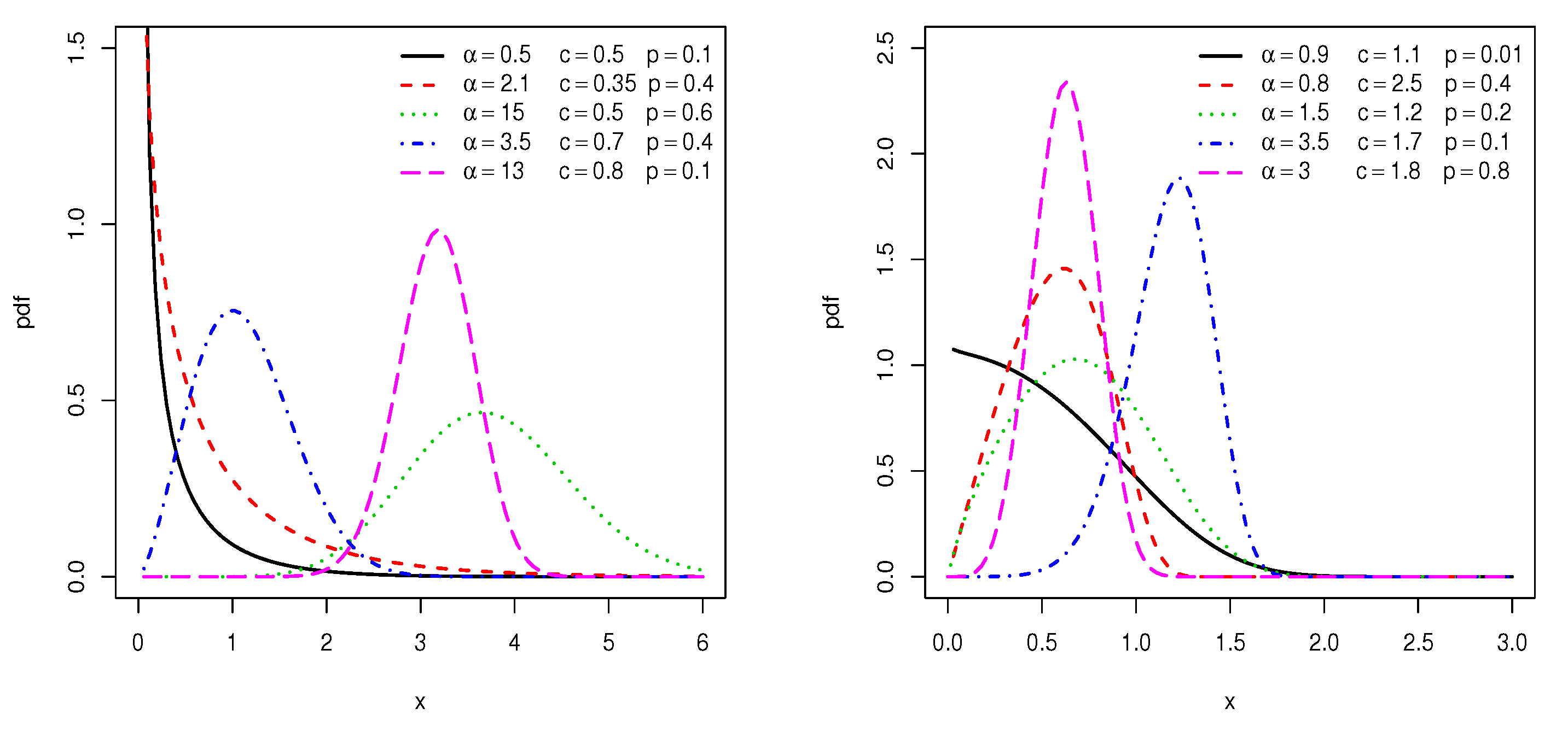
2.1. Main Probability Functions

Let us recall that the cdf of the OGWG distribution is defined by (1) with $G(x)$ given (2). By noticing that ${\mathrm{odd}}_{\mathrm{G}}(x)=(e^{{(\beta x)}^c}-1)/(1-p)$, the corresponding cdf is given by

$$F(x)=\frac{1}{\Gamma (\alpha )}\gamma \left(\alpha ,\frac{e^{{(\beta x)}^c}-1}{1-p}\right),x>0,$$

(3)

with $c>0$, $\alpha >0$, $p\in [0,1)$ and $\beta >0$. When needed, the OGWG distribution will be denoted by $OGWG(c,\alpha ,p,\beta )$ in order to specify the parameters. By differentiation (almost surely), the pdf corresponding to (3) is given by

$$f(x)=\frac{c{\beta }^c}{\Gamma (\alpha ){(1-p)}^{\alpha }}{x}^{c-1}{e}^{{(\beta x)}^c}{\left(e^{{(\beta x)}^c}-1\right)}^{\alpha -1}exp\left(\frac{1-e^{{(\beta x)}^c}}{1-p}\right),x>0.$$

(4)

The survival function of the OGWG distribution is given by

$$S(x)=1-F(x)=1-\frac{1}{\Gamma (\alpha )}\gamma \left(\alpha ,\frac{e^{{(\beta x)}^c}-1}{1-p}\right),x>0.$$

The corresponding hazard rate function (hrf) is given by

$$\begin{array}{cc}\hfill h(x)& =\frac{f(x)}{S(x)}\hfill \\ & =\frac{c{\beta }^c{x}^{c-1}{e}^{{(\beta x)}^c}}{{(1-p)}^{\alpha }\left\{\Gamma (\alpha )-\gamma \left(\alpha ,(e^{{(\beta x)}^c}-1)/(1-p)\right)\right\}}{\left(e^{{(\beta x)}^c}-1\right)}^{\alpha -1}exp\left(\frac{1-e^{{(\beta x)}^c}}{1-p}\right),x>0.\hfill \end{array}$$

(5)

Remark 1.

One can remark that he OGWG distribution is special case of the general gamma-Weibull-Weibull distribution introduced by ([7], Section 6) (with the notations of [7], it corresponds to $\beta =1$, simplifying the complexity of the distribution, $\alpha =1/(1-p)$, $\lambda =1/\beta$ and $k=c$). It is also an extension of the so-called exponentiated exponential power distribution thanks to the presence of the parameter p.

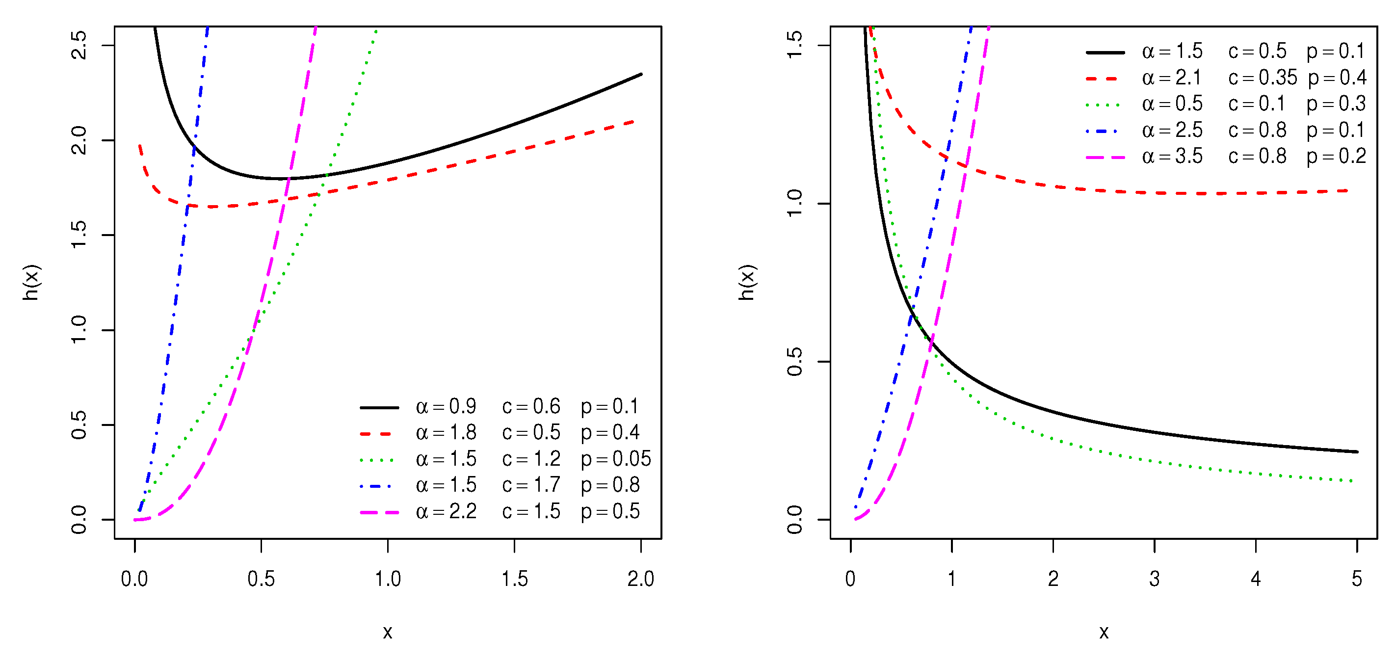
2.2. Analytical Properties of the Shapes

We now investigate the critical points and asymptotes for the OGWG pdf, i.e., $f(x)$ given by (4), and the OGWG hrf, i.e., $h(x)$ given by (5). In order to deal with tractable equations for the critical points, we work with the logarithmic functions: $log[f(x)]$ and $log[h(x)]$. Thus, the critical points of $f(x)$ are the solution $x_0$ of the nonlinear equation $\partial log[f(x)]/\partial x{\mid }_{x=x_0}=0$, i.e.,

$$\begin{array}{c}(c-1)\frac{1}{x_0}+c{\beta }^c{x}_0^{c-1}+c{\beta }^c{x}_0^{c-1}{e}^{{(\beta x_0)}^c}\left\{(\alpha -1)\frac{1}{e^{{(\beta x_0)}^c}-1}-\frac{1}{1-p}\right\}=0.\hfill \end{array}$$

The nature of $x_0$ can be determined by the study of the sign of the value ${\partial }^{2}log[f(x)]/\partial x^2{\mid }_{x=x_0}$. For given parameters c, $\alpha$, p and $\beta$, this aspect can be evaluated numerically by using a standard software (R, Matlab, Mathematica…).

In a similar way, the critical points of $h(x)$ are the solution $x_{*}$ of the nonlinear equation $\partial log[h(x)]/\partial x{\mid }_{x=x_{*}}=0$, i.e.,

$$\begin{array}{c}(c-1)\frac{1}{x_{*}}+c{\beta }^c{x}_{*}^{c-1}+c{\beta }^c{x}_{*}^{c-1}{e}^{{(\beta x_{*})}^c}\times \hfill \\ \left\{(\alpha -1)\frac{1}{e^{{(\beta x_{*})}^c}-1}-\frac{1}{1-p}+\frac{{\left(e^{{(\beta x_{*})}^c}-1\right)}^{\alpha -1}exp\left((1-e^{{(\beta x_{*})}^c})/(1-p)\right)}{{(1-p)}^{\alpha }\left\{\Gamma (\alpha )-\gamma \left(\alpha ,(e^{{(\beta x_{*})}^c}-1)/(1-p)\right)\right\}}\right\}=0.\hfill \end{array}$$

Again, the nature of $x_{*}$ can be determined by the study of the sign of the value ${\partial }^{2}log[h(x)]/\partial x^2{\mid }_{x=x_0}$.

The asymptotic properties of $F(x)$, $f(x)$ and $h(x)$ are now studied. Since $\gamma (\alpha ,u)\sim u^{\alpha }/\alpha$ when $u\to 0$, for $x\to 0$, we have

$$F(x)\sim \frac{1}{\alpha \Gamma (\alpha )}\frac{{\beta }^{\alpha c}}{{(1-p)}^{\alpha }}{x}^{\alpha c},f(x)\sim \frac{c{\beta }^{\alpha c}}{\Gamma (\alpha ){(1-p)}^{\alpha }}{x}^{\alpha c-1},h(x)\sim \frac{c{\beta }^{\alpha c}}{\Gamma (\alpha ){(1-p)}^{\alpha }}{x}^{\alpha c-1}.$$

In this case, note that $f(x)$ tends to 0 when $\alpha c>1$, tends to $\beta /[\alpha \Gamma (\alpha ){(1-p)}^{\alpha }]$ when $\alpha c=1$ and tends to $+\infty$ when $\alpha c\in (0,1)$. The same results hold for $h(x)$.

Since $\gamma (\alpha ,u)\sim \Gamma (\alpha )-u^{\alpha -1}{e}^{-u}$ when $u\to +\infty$, for $x\to +\infty$, we have

$$F(x)\sim 1-\frac{1}{\Gamma (\alpha )}\frac{1}{{(1-p)}^{\alpha -1}}{e}^{(\alpha -1){(\beta x)}^c}exp\left(\frac{1-e^{{(\beta x)}^c}}{1-p}\right),$$

$$f(x)\sim \frac{c{\beta }^c}{\Gamma (\alpha ){(1-p)}^{\alpha }}{x}^{c-1}{e}^{\alpha {(\beta x)}^c}exp\left(\frac{1-e^{{(\beta x)}^c}}{1-p}\right)$$

and

$$h(x)\sim \frac{c{\beta }^c}{1-p}{x}^{c-1}{e}^{{(\beta x)}^c}.$$

Let us remark that, in this case, $f(x)$ tends to 0, whereas $h(x)$ tends to $+\infty$, for all the possible values of the parameters. Also, the parameter $\alpha$ plays no role in the asymptotic behavior of $h(x)$.

Figure 1 and Figure 2 display some plots of $f(x)$ and $h(x)$ when $\beta =1$ for different values of c, $\alpha$ and p. The plots in Figure 1 reveal that $f(x)$ can have reversed-J, right skewed shapes, left-skewed and approximately symmetric. The plots in Figure 2 indicate that the $h(x)$ can have increasing failure rate, decreasing failure rate and bathtub shapes.

3. Some Mathematical Properties of the OGWG Distribution

3.1. Quantile Function

The quantile function of the OGWG distribution, denoted by $Q(y)$, $y\in (0,1)$, is characterized by the non-linear equation: $F(Q(y))=y$. After some algebra, we obtain

$$\begin{array}{c}\hfill Q(y)=\frac{1}{\beta }{\left[log\left\{1+(1-p){\gamma }^{-1}(\alpha ,y\Gamma (\alpha ))\right\}\right]}^{1/c},y\in (0,1),\end{array}$$

(6)

where ${\gamma }^{-1}(\alpha ,x)$ is the inverse lower incomplete gamma function, i.e., satisfying ${\gamma }^{-1}(\alpha ,\gamma (\alpha ,x))=x$ for $x>0$. The median of the OGWG distribution is given by $M_{*}=Q(0.5)$. For $i\in \{1,2,3\}$, the i-th quartile is given by $Q_i=Q(i/4)$ (with $Q_2=M_{*}$) and for $j\in \{1,\dots ,7\}$, the j-th octile is given by $E_j=Q(j/8)$.

Among others, we can use the quartiles and the octiles to investigate the effect of the parameters c, $\alpha$, p and $\beta$ on the skewness and kurtosis of the OGWG distribution. One of the earliest skewness measure is the Bowley skewness introduced by [9] and defined by

$$B=\frac{Q_3+Q_1-2Q_2}{Q_3-Q_1}.$$

For the kurtosis, one can use the Moors kurtosis introduced by [10] and defined by

$$M=\frac{E_3-E_1+E_7-E_5}{E_6-E_2}.$$

The sign of B is informative on the skewness nature of the distribution. Indeed, if $B=0$ then the distribution is symmetric, if $B>0$ then the distribution has a right skewed tail and if $B<0$ then the distribution has a left skewed tail. On the other side, the heaviness of the tail is evaluated numerically by M. A large M corresponds to a heavy tail.

Also, we can derive the quantile density function by differentiation of $Q(y)$. It comes

$$\begin{array}{cc}\hfill q(y)& =\frac{1}{f(Q(y))}=\frac{1}{\beta c}{\left[log\left\{1+(1-p){\gamma }^{-1}(\alpha ,y\Gamma (\alpha ))\right\}\right]}^{1/c-1}\times \hfill \\ & \frac{(1-p)\Gamma (\alpha )}{\left[1+(1-p){\gamma }^{-1}(\alpha ,y\Gamma (\alpha ))\right]{({\gamma }^{-1}(\alpha ,y\Gamma (\alpha )))}^{\alpha -1}{e}^{-{\gamma }^{-1}(\alpha ,y\Gamma (\alpha ))}},y\in (0,1).\hfill \end{array}$$

This function is useful to defined numerous statistical quantities (asymptotic confidence intervals, inference procedures…). We refer to [11].

3.2. Some Characterizations

Let U be a random variable following the uniform distribution over $(0,1)$ and $Q(y)$ be the quantile function given by (6). Then, the random variable X defined by

$$X=Q(U)=\frac{1}{\beta }{\left[log\left\{1+(1-p){\gamma }^{-1}(\alpha ,U\Gamma (\alpha ))\right\}\right]}^{1/c}$$

follows the $OGWG(c,\alpha ,p,\beta )$ distribution. By noticing that $Z={\gamma }^{-1}(\alpha ,U\Gamma (\alpha ))$ follows the gamma distribution with parameters 1 and $\alpha$, i.e., with cdf $R(x)=(1/\Gamma (\alpha )){\int }_0^x{t}^{\alpha -1}{e}^{-t}dt$, $x>0$, one can also write X according to Z as $X=(1/\beta ){\left[log\left\{1+(1-p)Z\right\}\right]}^{1/c}$. This characterization is useful to generate data according to the $OGWG(c,\alpha ,p,\beta )$ distribution.

Furthermore, if X is a random variable following the $OGWG(c,\alpha ,p,\beta )$ distribution, then the random variable Y defined by

$$Y=\frac{e^{{(\beta X)}^c}-1}{1-p}$$

follows the gamma distribution with parameters 1 and $\alpha$.

3.3. Series Expansion of the OGWG pdf

The following result presents a series expansion for the OGWG pdf.

Proposition 1.

The OGWG pdf can be expressed as sums of Weibull pdfs. More precisely, there exists a sequence of real number ${(v_{r,s})}_{(r,s)\in {\mathbb{N}}^2}$ such that the pdf $f(x)$ given by can be expressed as

$$f(x)=\sum _{r,s=0}^{+\infty }{v}_{r,s}{\ell }_{r,s}(x),$$

where ${\ell }_{r,s}(x)=c(r+s+1){\beta }^c{x}^{c-1}{e}^{-(r+s+1){(\beta x)}^c}$ and one can remark that ${\ell }_{r,s}(x)$ is the pdf of the Weibull distribution with parameters ${(r+s+1)}^{1/c}\beta$ and c.

Proof. 

Let us consider the expression of $f(x)$ depending on $G(x)$ and $g(x)$, i.e.,

$$f(x)=\frac{1}{\Gamma (\alpha )}\frac{g(x)}{{\left[\overline{G}(x)\right]}^2}{\left[\frac{G(x)}{\overline{G}(x)}\right]}^{\alpha -1}exp\left\{-\frac{G(x)}{\overline{G}(x)}\right\},x\in \mathbb{R},$$

with $G(x)=(1-e^{-{(\beta x)}^c})/(1-p{e}^{-{(\beta x)}^c})$ and $g(x)=c{\beta }^c(1-p)x^{c-1}{e}^{-{(\beta x)}^c}{\left[1-p{e}^{-{(\beta x)}^c}\right]}^{-2}$.

By virtue of the power series expansion of the exponential function, i.e., $e^x={\displaystyle \sum _{i=0}^{+\infty }}\frac{1}{i!}{x}^i$, $x\in \mathbb{R}$, and the generalized binomial series expansion, i.e., ${(1-x)}^b={\displaystyle \sum _{j=0}^{+\infty }}\left(\genfrac{}{}{0pt}{}{b}{j}\right){(-1)}^j{x}^j$, $\left|x\right|<1$, where $\left(\genfrac{}{}{0pt}{}{b}{j}\right)=b(b-1)\dots (b-j+1)/j!$, $f(x)$ can be expressed as

$$\begin{array}{cc}\hfill f(x)& =\frac{1}{\Gamma (\alpha )}\frac{g(x)}{{\left[\overline{G}(x)\right]}^2}{\left[\frac{G(x)}{\overline{G}(x)}\right]}^{\alpha -1}\sum _{i=0}^{+\infty }\frac{{(-1)}^i}{i!}{\left[\frac{G(x)}{\overline{G}(x)}\right]}^i\hfill \\ & =\frac{1}{\Gamma (\alpha )}\sum _{i=0}^{+\infty }\frac{{(-1)}^i}{i!}g(x){[G(x)]}^{\alpha +i-1}{[1-G(x)]}^{-\alpha -i-1}\hfill \\ & =\frac{1}{\Gamma (\alpha )}\sum _{i,j=0}^{+\infty }\left(\genfrac{}{}{0pt}{}{-\alpha -i-1}{j}\right)\frac{{(-1)}^{i+j}}{i!}g(x){\left[G(x)\right]}^{\alpha +i+j-1}\hfill \\ & =\frac{1}{\Gamma (\alpha )}\sum _{i,j=0}^{+\infty }\left(\genfrac{}{}{0pt}{}{-\alpha -i-1}{j}\right)\frac{{(-1)}^{i+j}}{i!}\left[c{\beta }^c(1-p)x^{c-1}{e}^{-{(\beta x)}^c}\right]\frac{{\left(1-e^{-{(\beta x)}^c}\right)}^{\alpha +i+j-1}}{{\left(1-p{e}^{-{(\beta x)}^c}\right)}^{\alpha +i+j+1}}.\hfill \end{array}$$

By applying the generalized binomial formula twice, we have

$$\begin{array}{cc}\hfill \frac{{\left(1-e^{-{(\beta x)}^c}\right)}^{\alpha +i+j-1}}{{\left(1-p{e}^{-{(\beta x)}^c}\right)}^{\alpha +i+j+1}}& =\sum _{r,s=0}^{+\infty }\left(\genfrac{}{}{0pt}{}{\alpha +i+j-1}{r}\right)\left(\genfrac{}{}{0pt}{}{-\alpha -i-j-1}{s}\right){(-1)}^{r+s}{p}^s{e}^{-(r+s){(\beta x)}^c}.\hfill \end{array}$$

Putting all the above equalities together, we get

$$\begin{array}{c}\hfill f(x)=\sum _{r,s=0}^{+\infty }{v}_{r,s}{\ell }_{r,s}(x),\end{array}$$

where

$$\begin{array}{c}\hfill v_{r,s}=(1-p)\frac{1}{r+s+1}\frac{1}{\Gamma (\alpha )}\sum _{i,j=0}^{+\infty }\left(\genfrac{}{}{0pt}{}{-\alpha -i-1}{j}\right)\left(\genfrac{}{}{0pt}{}{\alpha +i+j-1}{r}\right)\left(\genfrac{}{}{0pt}{}{-\alpha -i-j-1}{s}\right){(-1)}^{r+s+i+j}{p}^s\frac{1}{i!}\end{array}$$

and ${\ell }_{r,s}(x)=c(r+s+1){\beta }^c{x}^{c-1}{e}^{-(r+s+1){(\beta x)}^c}$. This ends the proof of Proposition 1. □

The result of Proposition 1 is useful to have sum expressions of various probability measures, specially those of the form ${\int }_{-\infty }^{+\infty }k(x)f(x)dx$, where $k(x)$ denotes a certain function. Indeed, when the dominated convergence theorem can be applied, we have the following series expansion:

$$\begin{array}{c}\hfill {\int }_{-\infty }^{+\infty }k(x)f(x)dx=\sum _{r,s=0}^{+\infty }{v}_{r,s}{\int }_0^{+\infty }k(x){\ell }_{r,s}(x)dx.\end{array}$$

(7)

3.4. Moments

Hereafter, X denotes a random variable following the $OGWG(c,\alpha ,p,\beta )$ distribution.

It follows from the asymptotic study of $f(x)$ performed in Section 2.2 that, for any integer m, m-th moment of X exists (by using Riemann integrals). Furthermore, it is given by

$$\begin{array}{cc}\hfill {\mu }_m^{\prime }& =\mathbb{E}(X^m)={\int }_{-\infty }^{+\infty }{x}^{m}f(x)dx\hfill \\ & =\frac{c{\beta }^c}{\Gamma (\alpha ){(1-p)}^{\alpha }}{\int }_0^{+\infty }{x}^{m+c-1}{e}^{{(\beta x)}^c}{\left(e^{{(\beta x)}^c}-1\right)}^{\alpha -1}exp\left(\frac{1-e^{{(\beta x)}^c}}{1-p}\right)dx.\hfill \end{array}$$

Several expressions of this integral are given below. First of all, by applying the natural change of variable $y=(e^{{(\beta x)}^c}-1)/(1-p)$, i.e., $x=(1/\beta ){[log(1+(1-p)y)]}^{1/c}$, we obtain

$$\begin{array}{c}\hfill {\mu }_m^{\prime }=\frac{1}{\Gamma (\alpha )}\frac{1}{{\beta }^m}{\int }_0^{+\infty }{[log(1+(1-p)y)]}^{m/c}{y}^{\alpha -1}{e}^{-y}dy.\end{array}$$

(8)

To the best of our knowledge, there is no closed form for this integral. However, for given parameters c, $\alpha$, p and $\beta$, it can be computed numerically by using a scientific softwares (see

Table 1. Some moments, variance, skewness and kurtosis of the $OGWG(c,\alpha ,p,\beta )$ distribution for the following selected parameters values in order $(c,\alpha ,p,\beta )$; (i): $(0.3,0.2,0.2,1)$, (ii): $(0.1,0.1,0.2,1)$, (iii): $(0.1,1,0.2,0.1)$ (iv): $(0.1,2,0.5,1)$ (v): $(0.1,5,0.5,1)$ and (vi): $(0.5,5,0.5,1)$.

	(i)	(ii)	(iii)	(iv)	(v)	(vi)
${\mu }_1^{\prime }$	0.0449	0.0472	3.0687	1.4307	12.8356	1.5471
${\mu }_2^{\prime }$	0.0674	1.5278	137.2844	44.8664	598.1401	2.9802
${\mu }_3^{\prime }$	0.2314	87.1821	8749.1190	12489.1710	38083.25	6.7361
${\mu }_4^{\prime }$	1.2680	6047.4790	640578.8	169843.6	2776370	17.2563
$\mathbb{V}(X)$	0.0654	1.5256	127.8670	42.8193	433.3854	0.5865
$CS$	13.3020	46.1489	5.2168	8.2173	2.13697	0.6909
$CK$	286.7989	2591.0480	33.0687	7.086025	3.3211	3.4358

below).

The following result proposes bounds for ${\mu }_m^{\prime }$. This gives an approximative analytical view on the roles of the parameters on the possible values of ${\mu }_m^{\prime }$.

Proposition 2.

Let us set

$$A_{c,\alpha ,p,\beta }=\frac{\Gamma (m/c+\alpha )}{\Gamma (\alpha )}\frac{{(1-p)}^{m/c}}{{\beta }^m}.$$

Then, we can bound ${\mu }_m^{\prime }$ as

$$\frac{1}{{[1+(m/c)(1-p)]}^{m/c+\alpha }}{A}_{c,\alpha ,p,\beta }\le {\mu }_m^{\prime }\le A_{c,\alpha ,p,\beta }.$$

Proof. 

Let us consider the expression (8) for ${\mu }_m^{\prime }$. The following bounds hold for the logarithmic function: for any $x>0$, $x/(1+x)\le log(1+x)\le x$. On the other hand, we have $e^x\ge 1+x$ for any $x\in \mathbb{R}$. Therefore, for any $x>0$, we have $x{e}^{-x}\le log(1+x)\le x$. Hence, by using $x{e}^{-x}\le log(1+x)$ and a change of variable, we obtain

$$\begin{array}{cc}\hfill {\mu }_m^{\prime }& \ge \frac{1}{\Gamma (\alpha )}\frac{1}{{\beta }^m}{\int }_0^{+\infty }{[(1-p)y{e}^{-(1-p)y}]}^{m/c}{y}^{\alpha -1}{e}^{-y}dy\hfill \\ & =\frac{1}{\Gamma (\alpha )}\frac{1}{{\beta }^m}{(1-p)}^{m/c}{\int }_0^{+\infty }{y}^{m/c+\alpha -1}{e}^{-[1+(m/c)(1-p)]y}dy\hfill \\ & =\frac{1}{\Gamma (\alpha )}\frac{1}{{\beta }^m}{(1-p)}^{m/c}\frac{1}{{[1+(m/c)(1-p)]}^{m/c+\alpha }}\Gamma (m/c+\alpha )\hfill \\ & =\frac{1}{{[1+(m/c)(1-p)]}^{m/c+\alpha }}{A}_{c,\alpha ,p,\beta }.\hfill \end{array}$$

In a similar way, by using $log(1+x)\le x$, we have

$$\begin{array}{cc}\hfill {\mu }_m^{\prime }& \le \frac{1}{\Gamma (\alpha )}\frac{1}{{\beta }^m}{\int }_0^{+\infty }{[(1-p)y]}^{m/c}{y}^{\alpha -1}{e}^{-y}dy\hfill \\ & =\frac{1}{\Gamma (\alpha )}\frac{1}{{\beta }^m}{(1-p)}^{m/c}{\int }_0^{+\infty }{y}^{m/c+\alpha -1}{e}^{-y}dy\hfill \\ & =\frac{1}{\Gamma (\alpha )}\frac{1}{{\beta }^m}{(1-p)}^{m/c}\Gamma (m/c+\alpha )=A_{c,\alpha ,p,\beta }.\hfill \end{array}$$

By combining the previous bounds, we end the proof of Proposition 2. □

Alternatively, one can use directly the quantile function given by (6). Indeed, by the change of variable $x=Q(y)$, we have

$${\mu }_m^{\prime }={\int }_0^1{[Q(y)]}^{m}dy=\frac{1}{{\beta }^m}{\int }_0^1{\left[log\left\{1+(1-p){\gamma }^{-1}(\alpha ,y\Gamma (\alpha ))\right\}\right]}^{m/c}dy.$$

In fact, it is equivalent to (8) with the change of variable $u=(1/\Gamma (\alpha ))\gamma (\alpha ,y)$ in (8), i.e., $y={\gamma }^{-1}(\alpha ,u\Gamma (\alpha ))$.

As a final approach, one can use the result of Proposition 1 and more specially, the result (7). Hereafter, let $X_{r,s}$ be a random variable following the Weibull distribution with parameters ${(r+s+1)}^{1/c}\beta$ and c, i.e., with the pdf given by ${\ell }_{r,s}(x)=c(r+s+1){\beta }^c{x}^{c-1}{e}^{-{[{(r+s+1)}^{1/c}\beta x]}^c}$, $x>0$. Then, we have

$$\begin{array}{c}\hfill {\mu }_m^{\prime }=\sum _{r,s=0}^{+\infty }{v}_{r,s}\mathbb{E}(X_{r,s}^m)=\frac{1}{{\beta }^m}\sum _{r,s=0}^{+\infty }{v}_{r,s}\frac{1}{{(r+s+1)}^{m/c}}\Gamma \left(\frac{m}{c}+1\right).\end{array}$$

From any of the above expressions of ${\mu }_m^{\prime }$, we can derive central measures as the mean of X given by $\mathbb{E}(X)={\mu }_1^{\prime }$, the variance of X given by $\mathbb{V}(X)={\mu }_2^{\prime }-{({\mu }_1^{\prime })}^2$ and the m-th central moment of X given by

$${\mu }_m=\mathbb{E}\left[{(X-{\mu }_1^{\prime })}^m\right]=\sum _{k=0}^m\frac{m!}{k!(m-k)!}{(-1)}^k{({\mu }_1^{\prime })}^k{\mu }_{m-k}^{\prime }.$$

We can also determine other standard measures as the coefficient of skewness and coefficient of kurtosis, respectively given by

$$CS=\frac{{\mu }_3}{{\mu }_2^{3/2}},CK=\frac{{\mu }_4}{{\mu }_2^2}.$$

Table 1 presents the numerical values of ${\mu }_1^{\prime }$, ${\mu }_2^{\prime }$, ${\mu }_3^{\prime }$, ${\mu }_4^{\prime }$, $\mathbb{V}(X)$, $CS$ and $CK$ for selected values of the parameters.

3.5. Moment Generating Function

The moment generating function of X is given by

$$\begin{array}{cc}\hfill M(t)& =\mathbb{E}(e^{tX})={\int }_{-\infty }^{+\infty }{e}^{tx}f(x)dx\hfill \\ & =\frac{c{\beta }^c}{\Gamma (\alpha ){(1-p)}^{\alpha }}{\int }_0^{+\infty }{e}^{tx}{x}^{c-1}{e}^{{(\beta x)}^c}{\left(e^{{(\beta x)}^c}-1\right)}^{\alpha -1}exp\left(\frac{1-e^{{(\beta x)}^c}}{1-p}\right)dx.\hfill \end{array}$$

It is well defined for $t\in \mathbb{R}$. By applying the change of variable $y=(e^{{(\beta x)}^c}-1)/(1-p)$, we can express $M(t)$ as

$$M(t)=\frac{1}{\Gamma (\alpha )}{\int }_0^{+\infty }{e}^{(t/\beta ){[log(1+(1-p)y)]}^{1/c}}{y}^{\alpha -1}{e}^{-y}dy.$$

Alternatively, by the change of variable $x=Q(y)$, we have

$$M(t)={\int }_0^1{e}^{tQ(y)}dy={\int }_0^1{e}^{(t/\beta ){\left[log\left\{1+(1-p){\gamma }^{-1}(\alpha ,y\Gamma (\alpha ))\right\}\right]}^{1/c}}dy.$$

For given parameters c, $\alpha$, p, $\beta$ and t, the integrals above can be computed numerically.

A series expansion of $M(t)$ can be derived from (7). Indeed, we have

$$\begin{array}{c}\hfill M(t)=\sum _{r,s=0}^{+\infty }{v}_{r,s}\mathbb{E}(e^{t{X}_{r,s}})=\sum _{r,s=0}^{+\infty }\sum _{m=0}^{+\infty }{v}_{r,s}\frac{t^m}{m!{\beta }^m{(r+s+1)}^{m/c}}\Gamma \left(\frac{m}{c}+1\right).\end{array}$$

As always, we have the following relations between the moments and the moment generating function:

$${\mu }_m^{\prime }=M^{(m)}(t){\mid }_{t=0},M(t)=\sum _{m=0}^{+\infty }\frac{t^m}{m!}{\mu }_m^{\prime }.$$

3.6. Incomplete Moments

Let ${\mathbf{1}}_A$ be the indicator function of over an event A. Then, the m-th incomplete moment of X is defined by

$$\begin{array}{cc}\hfill {\theta }_m^{\prime }(t)& =\mathbb{E}\left(X^m{\mathbf{1}}_{\{X\le t\}}\right)={\int }_{-\infty }^t{x}^{m}f(x)dx\hfill \\ & ={\int }_0^t{x}^{m+c-1}{e}^{{(\beta x)}^c}{\left(e^{{(\beta x)}^c}-1\right)}^{\alpha -1}exp\left(\frac{1-e^{{(\beta x)}^c}}{1-p}\right)dx.\hfill \end{array}$$

By applying the change of variable $y=(e^{{(\beta x)}^c}-1)/(1-p)$, we obtain

$${\theta }_m^{\prime }(t)=\frac{1}{\Gamma (\alpha )}\frac{1}{{\beta }^m}{\int }_0^{(e^{{(\beta t)}^c}-1)/(1-p)}{[log(1+(1-p)y)]}^{m/c}{y}^{\alpha -1}{e}^{-y}dy.$$

One can determined bounds for ${\theta }_m^{\prime }(t)$ by proceeding as in the proof of Proposition 2.

Alternatively, by the change of variable $x=Q(y)$, we have immediately

$$\begin{array}{cc}\hfill {\theta }_m^{\prime }(t)& ={\int }_0^{F(t)}{[Q(y)]}^{m}dy\hfill \\ & =\frac{1}{{\beta }^m}{\int }_0^{\frac{1}{\Gamma (\alpha )}\gamma \left(\alpha ,(e^{{(\beta t)}^c}-1)/(1-p)\right)}{\left[log\left\{1+(1-p){\gamma }^{-1}(\alpha ,y\Gamma (\alpha ))\right\}\right]}^{m/c}dy.\hfill \end{array}$$

Again, for given parameters c, $\alpha$, p, $\beta$ and t, we can evaluate these integrals numerically.

Also, another expression comes from (7). We have

$$\begin{array}{c}\hfill {\theta }_m^{\prime }(t)=\sum _{r,s=0}^{+\infty }{v}_{r,s}\mathbb{E}\left(X_{r,s}^m{\mathbf{1}}_{\{X_{r,s}\le t\}}\right)=\frac{1}{{\beta }^m}\sum _{r,s=0}^{+\infty }{v}_{r,s}\frac{1}{{(r+s+1)}^{m/c}}\gamma \left(\frac{m}{c}+1,(r+s+1){(\beta t)}^c\right).\end{array}$$

With the first incomplete moment of X, one can define several kinds of means deviation. For instance, there are the mean deviation of X about the mean ${\mu }_1^{\prime }$ given by

$${\delta }_1=\mathbb{E}(|X-{\mu }_1^{\prime }|)=2{\mu }_1^{\prime }F({\mu }_1^{\prime })-2{\theta }_1^{\prime }({\mu }_1^{\prime })$$

and the mean deviation of X about the median $M_{*}$ given by

$${\delta }_2=\mathbb{E}(|X-M_{*}|)={\mu }_1^{\prime }-2{\theta }_1^{\prime }(M_{*}).$$

We can also express the Bonferroni and Lorenz curves respectively given by

$$B(y)=\frac{1}{y{\mu }_1^{\prime }}{\theta }_1^{\prime }(Q(y))=\frac{1}{y{\mu }_1^{\prime }}{\theta }_1^{\prime }\left(\frac{1}{\beta }{\left[log\left\{1+(1-p){\gamma }^{-1}(\alpha ,y\Gamma (\alpha ))\right\}\right]}^{1/c}\right)$$

and

$$L(y)=\frac{1}{{\mu }_1^{\prime }}{\theta }_1^{\prime }(Q(y))=\frac{1}{{\mu }_1^{\prime }}{\theta }_1^{\prime }\left(\frac{1}{\beta }{\left[log\left\{1+(1-p){\gamma }^{-1}(\alpha ,y\Gamma (\alpha ))\right\}\right]}^{1/c}\right),y\in (0,1).$$

As an example of the use of higher orders of the incomplete moments, the m-th moment of the residual life of X is given by

$$\begin{array}{cc}\hfill {\theta }_m^{*}(t)& =\frac{1}{1-F(t)}{\int }_t^{+\infty }{(x-t)}^{m}f(x)dx\hfill \\ & =\frac{\Gamma (\alpha )}{\Gamma (\alpha )-\gamma \left(\alpha ,(e^{{(\beta t)}^c}-1)/(1-p)\right)}\sum _{i=0}^m\left(\genfrac{}{}{0pt}{}{m}{i}\right){(-1)}^{m-i}{t}^{m-i}\left[{\mu }_i^{\prime }-{\theta }_i^{\prime }(t)\right],t\ge 0.\hfill \end{array}$$

3.7. Stochastic Ordering

Under some assumptions on the parameters, the result below shows that the $OGWG(c,\alpha ,p,\beta )$ distribution is ordered with respect to the likelihood ratio ordering. Further details and applications on stochastic ordering can be found in [12].

Proposition 3.

Let X be a random variable following the $OGWG(c,{\alpha }_1,p_1,\beta )$ distribution and Y be a random variable following the $OGWG(c,{\alpha }_2,p_2,\beta )$ distribution. Suppose that ${\alpha }_1\le {\alpha }_2$ and $p_2\le p_1$. Then X is smaller than Y in the likelihood ratio order, i.e., the function defined by ratio of the pdf of X over the pdf of Y is decreasing.

Proof. 

Let $f_1(x)$ be the pdf of X and $f_2(x)$ be the pdf of Y. Then, we have

$$\frac{f_1(x)}{f_2(x)}=\frac{\Gamma ({\alpha }_2){(1-p_2)}^{{\alpha }_2}}{\Gamma ({\alpha }_1){(1-p_1)}^{{\alpha }_1}}{\left(e^{{(\beta x)}^c}-1\right)}^{{\alpha }_1-{\alpha }_2}exp\left\{\frac{p_1-p_2}{(1-p_1)(1-p_2)}\left(1-e^{{(\beta x)}^c}\right)\right\}.$$

Let us consider the logarithmic function to have a more tractable expression. We have

$$\begin{array}{cc}\hfill log\left[\frac{f_1(x)}{f_2(x)}\right]& =log\left[\frac{\Gamma ({\alpha }_2){(1-p_2)}^{{\alpha }_2}}{\Gamma ({\alpha }_1){(1-p_1)}^{{\alpha }_1}}\right]\hfill \\ & +({\alpha }_1-{\alpha }_2)log\left(e^{{(\beta x)}^c}-1\right)+\frac{p_1-p_2}{(1-p_1)(1-p_2)}\left(1-e^{{(\beta x)}^c}\right).\hfill \end{array}$$

Since ${\alpha }_1\le {\alpha }_2$ and $p_2\le p_1$, as sum of two negative functions, we have

$$\begin{array}{cc}\hfill \frac{\partial }{\partial x}log\left[\frac{f_1(x)}{f_2(x)}\right]& =({\alpha }_1-{\alpha }_2)\frac{c{\beta }^c{x}^{c-1}{e}^{{(\beta x)}^c}}{e^{{(\beta x)}^c}-1}+\frac{p_2-p_1}{(1-p_1)(1-p_2)}c{\beta }^c{x}^{c-1}{e}^{{(\beta x)}^c}\le 0.\hfill \end{array}$$

The proof of Proposition 3 is completed. □

4. Estimation of Parameters

Hereafter, we focus our attention on the applied aspect of the OGWG distribution, considering it as a statistical model. Indeed, motivated by its flexibility discussed in the above sections, the OGWG model is appropriate for the analyses of data sets with a non-trivial structure, as those frequently encountered in engineering, medicine, hydrology, economics and finance.

4.1. Maximum Likelihood Estimation

Several parameter estimation methods are available in the literature. Among them, thanks to its strong theoretical guaranties, the maximum likelihood method remains the most popular. In particular, it can be used to construct confidence intervals for the model parameters and also in test statistics. For these reasons, we consider the estimation of the unknown parameters for the OGWG model from complete samples with this method only. Let $x_1,\dots ,x_n$ be a sample of size n from the $OGWG(c,\alpha ,p,\beta )$ distribution. The log-likelihood function for the vector of parameters $\Theta ={(c,\alpha ,p,\beta )}^{\top }$ is given by

$$\begin{array}{cc}\hfill \ell (\Theta )& =\sum _{i=1}^{n}log[f(x_i)]\hfill \\ & =nlog(c)+nclog(\beta )-nlog[\Gamma (\alpha )]-n\alpha log(1-p)+(c-1)\sum _{i=1}^{n}log(x_i)+\sum _{i=1}^n{(\beta x_i)}^c\hfill \\ & +(\alpha -1)\sum _{i=1}^{n}log\left(e^{{(\beta x_i)}^c}-1\right)+\frac{1}{1-p}\sum _{i=1}^n\left(1-e^{{(\beta x_i)}^c}\right).\hfill \end{array}$$

The corresponding score vector is given by $U(\Theta )={(U_c(\Theta ),U_{\alpha }(\Theta ),U_p(\Theta ),U_{\beta }(\Theta ))}^{\top }$ with

$$\begin{array}{cc}\hfill U_c(\Theta )& =\frac{\partial }{\partial c}\ell (\Theta )=\frac{n}{c}+nlog(\beta )+\sum _{i=1}^{n}log(x_i)+\sum _{i=1}^n{(\beta x_i)}^{c}log(\beta x_i)+(\alpha -1)\sum _{i=1}^n\frac{{(\beta x_i)}^{c}log(\beta x_i)e^{{(\beta x_i)}^c}}{e^{{(\beta x_i)}^c}-1}\hfill \\ & -\frac{1}{1-p}\sum _{i=1}^n{(\beta x_i)}^{c}log(\beta x_i)e^{{(\beta x_i)}^c},\hfill \\ \hfill U_{\alpha }(\Theta )& =\frac{\partial }{\partial \alpha }\ell (\Theta )=-n\frac{{\Gamma }^{\prime }(\alpha )}{\Gamma (\alpha )}-nlog(1-p)+\sum _{i=1}^{n}log\left(e^{{(\beta x_i)}^c}-1\right),\hfill \\ \hfill U_p(\Theta )& =\frac{\partial }{\partial p}\ell (\Theta )=\frac{n\alpha }{1-p}+\frac{1}{{(1-p)}^2}\sum _{i=1}^n\left(1-e^{{(\beta x_i)}^c}\right),\hfill \\ \hfill U_{\beta }(\Theta )& =\frac{\partial }{\partial \beta }\ell (\Theta )=\frac{nc}{\beta }+\frac{c}{\beta }\sum _{i=1}^n{(\beta x_i)}^c+\frac{c(\alpha -1)}{\beta }\sum _{i=1}^n\frac{{(\beta x_i)}^c{e}^{{(\beta x_i)}^c}}{e^{{(\beta x_i)}^c}-1}-\frac{c}{\beta (1-p)}\sum _{i=1}^n{(\beta x_i)}^c{e}^{{(\beta x_i)}^c}.\hfill \end{array}$$

By solving the system $U(\Theta )={(0,0,0,0)}^{\top }$, we obtain a solution denoted by $\widehat{\Theta }={(\widehat{c},\widehat{\alpha },\widehat{p},\widehat{\beta })}^{\top }$ (assuming that it is unique). Hence, $\widehat{c}$, $\widehat{\alpha }$, $\widehat{p}$ and $\widehat{\beta }$ are the maximum likelihood estimates (MLEs) of c, $\alpha$, p and $\beta$, respectively. The analytical expressions of these estimates do not exist in our case. However, they can be solved numerically by using iterative techniques (quasi-Newton BFGS, Newton-Raphson algorithms…). Further details can be found in [13]. Assuming that the parameters are in the interior of the parameter space but not on the boundary, the subjacent distribution of $\widehat{\Theta }$ can be approximated by a 4 dimensional normal distribution with mean $\Theta$ and covariance matrix given by $J{(\widehat{\Theta })}^{-1}$, where $J(\Theta )$ denotes the $4\times 4$ symmetric matrix defined by

$$\begin{array}{c}\hfill J(\Theta )=-\frac{{\partial }^2}{\partial \Theta \partial {\Theta }^T}\ell (\Theta )=-\left(\begin{array}{cccc}{l}_{c,c}& l_{c,\alpha }& l_{c,p}& l_{c,\beta }\\ .& l_{\alpha ,\alpha }& l_{\alpha ,p}& l_{\alpha ,\beta }\\ .& .& l_{p,p}& l_{p,\beta }\\ .& .& .& l_{\beta ,\beta }\end{array}\right),\end{array}$$

(9)

whose elements are given in Appendix A. From this asymptotic property, one can construct approximate confidence intervals for c, $\alpha$, p and $\beta$. More precisely, for $h\in \{c,\alpha ,p,\beta \}$, an approximate confidence interval for h at the level $100(1-\omega )\%$ is given by

$$\begin{array}{c}\hfill C{I}_h=[\widehat{h}-z_{\omega /2}{s}_{\widehat{h}},\widehat{h}+z_{\omega /2}{s}_{\widehat{h}}],\end{array}$$

(10)

where $s_{\widehat{h}}$ is the square-root of the diagonal element of $J{(\widehat{\Theta })}^{-1}$ at the same position as h and $z_{\omega /2}$ is the quantile $100(1-\omega /2)\%$ of the standard normal distribution. Also, we are able to compute the likelihood ratio (LR) statistics for testing goodness-of-fit of the OGWG model with its sub-models.

4.2. Monte Carlo Simulation Study

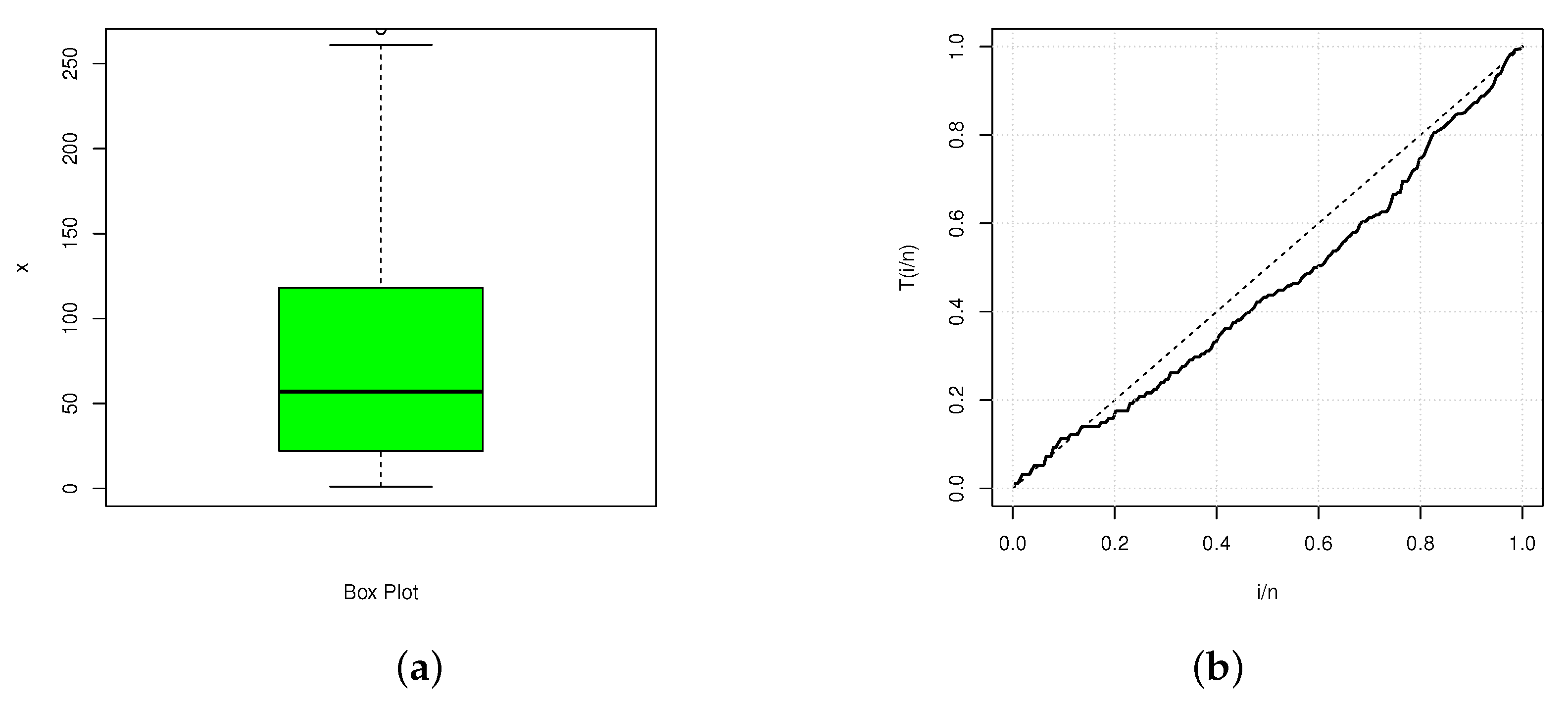
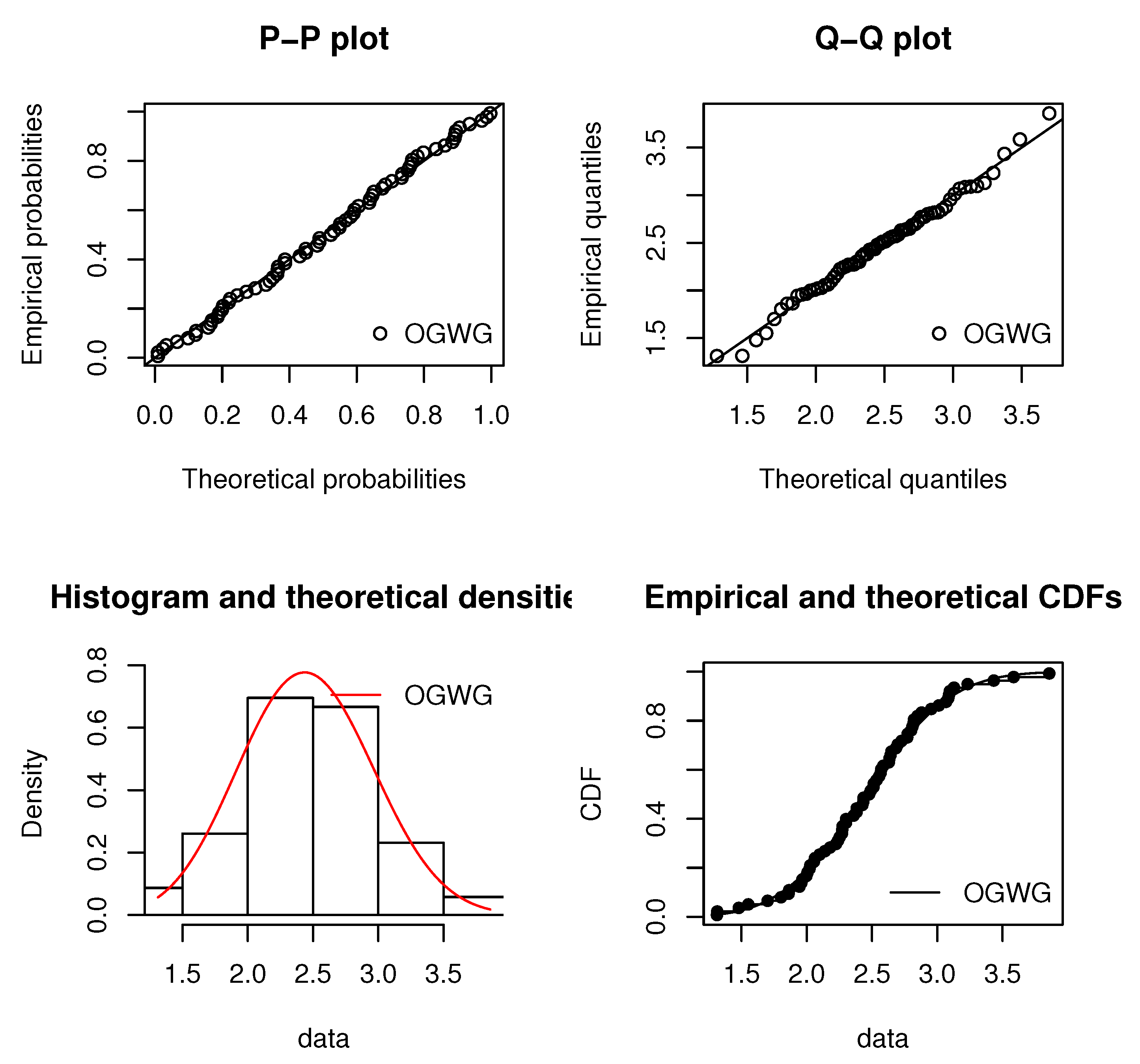
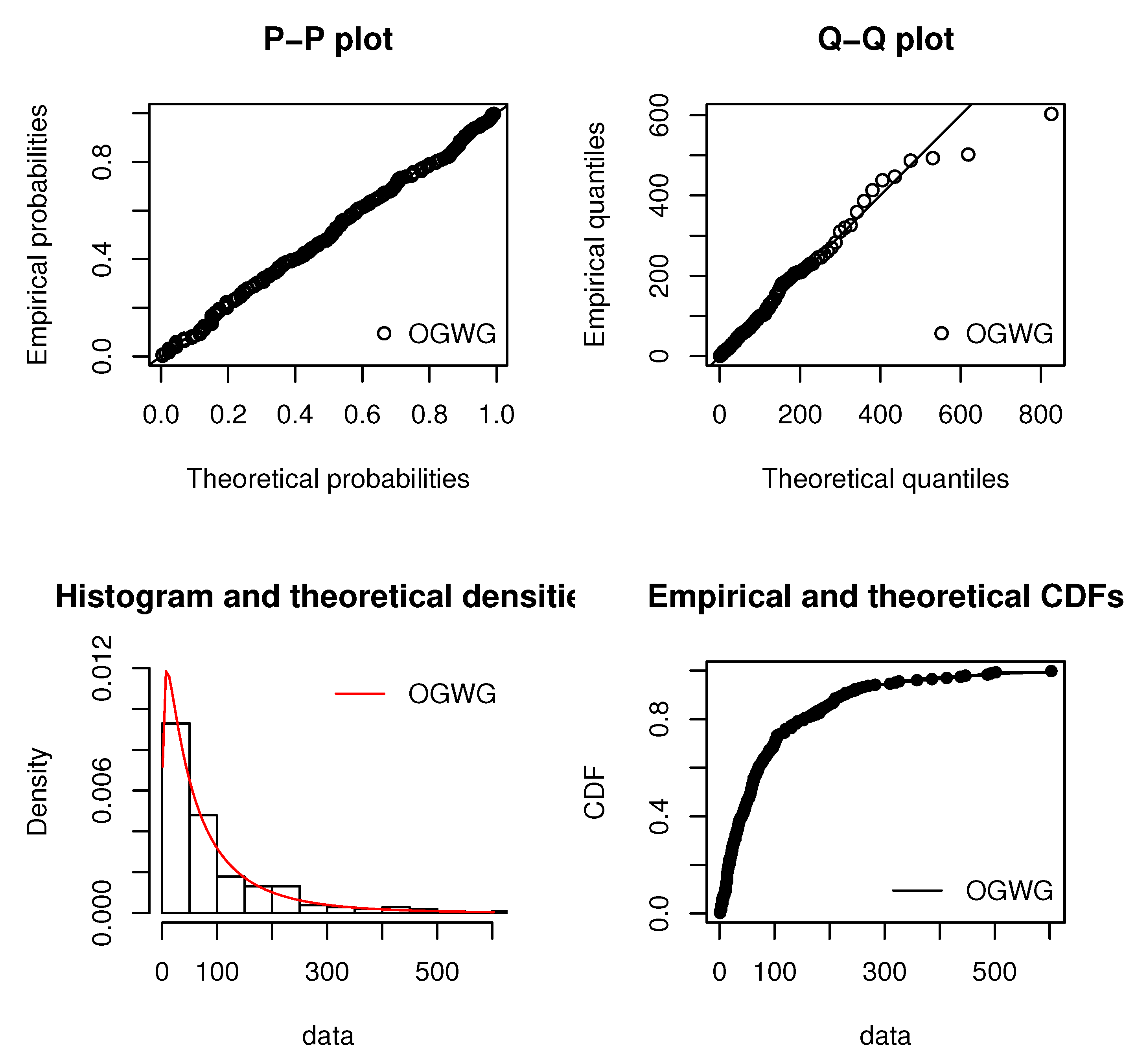
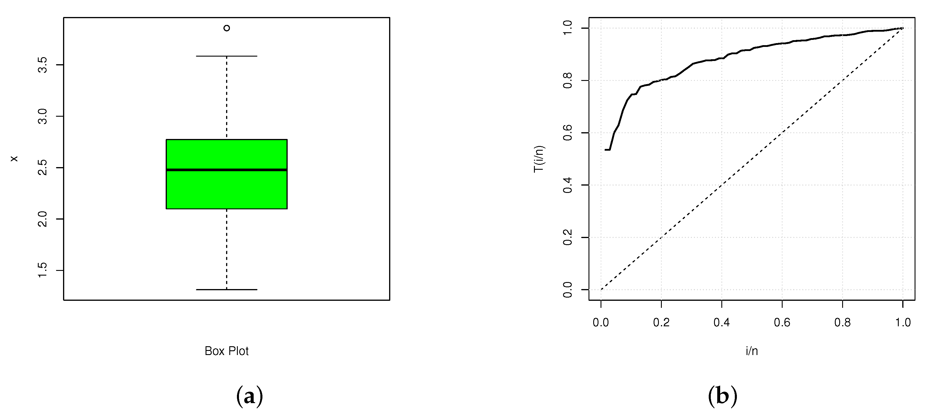
Now we assess the asymptotic properties of the MLEs for the parameters of the OGWG model using Monte Carlo simulations. The simulation study is repeated $N=5000$ times each with sample sizes $n=50$, 100, 200 and with the following parameter scenarios: I: $c=1.5$, $\alpha =0.5$, $p=0.5$ and $\beta =0.5$, II: $c=1.5$, $\alpha =0.5$, $p=0.1$ and $\beta =0.5$ and III: $c=1.5$, $\alpha =1.5$, $p=0.5$ and $\beta =0.8$. We investigate the empirical bias (Bias), mean square error (MSE) and coverage probability (CP) at the nominal level 95%. For $h\in \{c,\alpha ,p,\beta \}$, they are respectively defined by

$$Bia{s}_h(n)=\frac{1}{N}\sum _{i=1}^N({\widehat{h}}_i-h),MS{E}_h(n)=\frac{1}{N}\sum _{i=1}^N{({\widehat{h}}_i-h)}^2,C{P}_h(n)=\frac{1}{N}\sum _{i=1}^N{\mathbf{1}}_{({\widehat{h}}_i-u{s}_{{\widehat{h}}_i},{\widehat{h}}_i+u{s}_{{\widehat{h}}_i})},$$

where ${\widehat{h}}_i$ denotes the MLE of h obtained at the i-th repetition of the simulation and $z_{0.975}$ is the quantile 97.5% of the standard normal distribution, i.e., $u=z_{0.975}\approx 1.95996$.

Table 2. Biases, MSEs and CPs of the simulation study.

			I			II			III
Parameter	$\mathit{n}$	Bias	MSE	CP	Bias	MSE	CP	Bias	MSE	CP
c	50	0.028	0.098	0.99	0.146	0.535	0.94	0.511	1.433	0.96
	100	0.011	0.043	0.97	0.164	0.309	0.95	0.374	0.871	0.95
	200	−0.008	0.021	0.96	0.195	0.228	0.97	0.089	0.313	0.98
$\alpha$	50	0.250	0.410	0.94	0.172	0.241	1.00	0.118	0.913	0.95
	100	0.104	0.351	0.95	0.053	0.065	0.96	0.091	0.403	0.98
	200	−0.091	0.182	0.96	0.001	0.031	0.97	0.016	0.048	0.97
p	50	0.002	0.072	0.96	0.311	0.163	0.99	0.053	0.171	0.97
	100	−0.025	0.062	0.98	0.271	0.132	0.95	0.050	0.121	0.96
	200	−0.082	0.049	0.97	0.222	0.100	0.96	0.020	0.065	0.95
$\beta$	50	0.258	0.912	0.95	−0.062	0.022	0.95	0.211	0.391	0.93
	100	0.150	0.627	0.96	−0.059	0.017	0.96	0.100	0.253	0.95
	200	0.088	0.414	0.97	−0.051	0.011	0.98	0.093	0.191	0.96

gives the values of these measures under the scenarios and different sample sizes as indicated above. In most of the cases, we see that the empirical biases tends to zero when n increases, the empirical MSEs decay toward zero as n increases and the empirical CPs are quite close to the level 95%. Thus, based on these simulation results, we conclude that the MLEs perform well in estimating c, $\alpha$, p and $\beta$. Therefore, the MLEs and their asymptotic results can be adopted for estimating and constructing approximate confidence intervals for c, $\alpha$, p and $\beta$.

5. Data Analysis

In this section, the OGWG distribution is used as model to analyze two a real-life data sets. We compare the fits of the OGWG model with the beta-Weibull (BW) (see [14]), Weibull-geometric (WG) (see [8]) and gamma-Weibull (GW) models (i.e., the OGWG model with $p=0$). The corresponding pdfs are respectively given by

$$\begin{array}{c}OGWG:f_{OGWG}(x)=\frac{c{\beta }^c}{\Gamma (\alpha ){(1-p)}^{\alpha }}{x}^{c-1}{e}^{{(\beta x)}^c}{\left(e^{{(\beta x)}^c}-1\right)}^{\alpha -1}exp\left(\frac{1-e^{{(\beta x)}^c}}{1-p}\right),x,c,\alpha ,p,\beta >0,\hfill \\ BW:f_{BW}(x)=\frac{c{\beta }^c{x}^{c-1}{e}^{-b{(\beta x)}^c}}{\Gamma (a)\Gamma (b)/\Gamma (a+b)}{\left(1-e^{-{(\beta x)}^c}\right)}^{a-1},x,a,b,c,\beta >0,\hfill \\ WG:f_{WG}(x)=\frac{1-e^{-{(\beta x)}^c}}{1-p{e}^{-{(\beta x)}^c}},x,c,p,\beta >0,\hfill \\ GW:f_{GW}(x)=\frac{c{\beta }^c}{\Gamma (\alpha )}{x}^{c-1}{e}^{{(\beta x)}^c}{\left(e^{{(\beta x)}^c}-1\right)}^{\alpha -1}exp\left(1-e^{{(\beta x)}^c}\right),x,\alpha ,c,\beta >0.\hfill \end{array}$$

We estimate the model parameters by using the maximum likelihood method as presented in Section 4. We compare the goodness-of-fit of the models using Cramér–von Mises ($W^{*}$) and Anderson-Darling ($A^{*}$) statistics, which are described in detail by [15]. In addition, we consider the Kolmogorov-Smirnov (K-S) statistic, AIC and BIC. In general, the smaller the values of these statistics, the better the fit to the data. Two analyses are performed on two different data sets, as described below.

Data analysis 1: The first data set, taken from [16], represents the failure times of air conditioning system of air plan. Some descriptive statistics are given in

Table 3. Descriptive statistics for data set 1.

Statistics	n	Mean	Median	Mode	Variance	Skewness	Kurtosis
Data 1	213	93.1408	57	14	106.76	2.1118	4.9249

. The skewness is positive (right-skewed data) and the kurtosis is positive. The boxplot and the TTT plot are given in Figure 3. In particular, the TTT plot shows a possible monotonically increasing or constant hrf, indicating that the OGWG model could be appropriate for the fitting of this data set. The MLEs (with SEs in parenthesis), $A^{*}$, $W^{*}$, K-S statistics, AIC and BIC are listed in

Table 4. MLEs, their SEs (in parentheses) and goodness-of-fit measures for data set 1.

Distribution	Estimates				${\mathit{A}}^{*}$	${\mathit{W}}^{*}$	K-S	AIC	BIC
$OGWG(c,\alpha ,p,\beta )$	0.1527	11.5290	0.8340	0.0249	0.2506	0.0338	0.0379	2353.8560	2363.0490
	(0.0520)	(2.4351)	(0.1133)	(0.0320)
$BW(a,b,c,\beta )$	3.6631	0.1333	0.6803	0.3258	0.2964	0.0383	0.0391	2357.3430	2370.7880
	(0.6564)	(0.0098)	(0.0025)	(0.0025)
$WG(c,p,\beta )$	1.1719	0.7071	0.0056		0.2957	0.0425	0.0390	2354.6050	2364.6890
	(0.0956)	(0.1196)	(0.0011)
$GW(\alpha ,c,\beta )$	0.2868	2.7657	0.0342		1.0608	0.1717	0.0573	2363.5300	2373.6140
	(0.0679)	(0.7995)	(0.0292)

. For each criterion, the smallest values is reached by the OGWG model, indicating that it provides the best fit. For a visual approach, the estimated pdf and cdf of the OGWG model are displayed in Figure 4. We also see the P-P and Q-Q plots. All the graphics show nice fits for the OGWG model. Finally, the asymptotic confidence intervals of the OGWG parameters given by (10) are presented in

Table 5. Confidence intervals of OGWG for data set 1.

CI	c	$\mathit{\alpha }$	p	$\mathit{\beta }$
95%	[0.0507 0.2546]	[6.7562 16.3017]	[0.6119 1.0560]	[0 0.0876]
99%	[0.0185 0.2868]	[5.2464 17.8115]	[0.5416 1.1263]	[0 0.1074]

with the levels 95% and 99%.

Data analysis 2: The second data set, taken from [17], represents the tensile strength, measured in GPa, of 69 carbon fibers tested under tension at gauge lengths of 20 mm. The summary statistics are given in

Table 6. Descriptive statistics for data set 2.

Statistics	n	Mean	Median	Mode	Variance	Skewness	Kurtosis
Data 2	69	2.4551	2.4780	2.2500	0.5052	0.1020	0.2253

. The skewness and kurtosis are positive but close to zero. Figure 5 shows the boxplot and the TTT plot. Since the curve in the TTT plot is concave, it seems to correspond to a monotonically decreasing hrf, so the OGWG model could be suitable for the fitting of data set 2. The MLEs (with SEs in parenthesis), $A^{*}$, $W^{*}$, K-S statistics, AIC and BIC are listed in

Table 7. MLEs, their SEs (in parentheses) and goodness-of-fit measures for data set 2.

Distribution	Estimates				${\mathit{A}}^{*}$	${\mathit{W}}^{*}$	K-S	AIC	BIC
$OGWG(c,\alpha ,p,\beta )$	1.8247	5.6103	0.9449	0.1931	0.1705	0.0188	0.0328	104.6965	111.6329
	(0.1062)	(1.1340)	(0.0898)	(0.1349)
$BW(a,b,c,\beta )$	2.6824	1.0947	3.2891	0.4510	0.1736	0.0211	0.0433	108.5069	117.4433
	(2.6516)	(3.4755)	(2.1102)	(0.2442)
$WG(c,p,\beta )$	7.5850	0.8884	0.3046		0.1899	0.0252	0.0423	106.5669	113.2692
	(1.1497)	(0.1321)	(0.0327)
$GW(\alpha ,c,\beta )$	0.5060	12.1478	2.5990		0.1810	0.0221	0.0443	106.5870	113.2894
	(0.4747)	(14.2268)	(6.7712)

. All are favorable to the OGWG model. Also, the estimated pdf and cdf of the OGWG model are displayed in Figure 6, as well as P-P and Q-Q plots. All the graphics show nice fits for the OGWG model. Finally, the asymptotic confidence intervals of the OGWG parameters given by (10) are presented in

Table 8. Confidence intervals of OGWG for data set 2.

CI	c	$\mathit{\alpha }$	p	$\mathit{\beta }$
95%	[1.6165 2.0328]	[3.3876 7.8329]	[0.7704 1.1193]	[0 0.4575]
99%	[1.5507 2.0986]	[2.6845 8.5360]	[0.7158 1.1745]	[0 0.5411]

with the levels 95% and 99%.

Among others, the obtained results of this data set suggest that the OGWG family of distributions can be also utilized in calibration and errors-in-variables modeling (see [18]).

6. Concluding Remarks

This paper proposed a new distribution called the odd gamma Weibull-geometric distribution (OGWG) and developed its merits from the mathematical and practical points of view. In particular, we study its shapes, asymptotes, quantile function, quantile density function, skewness, kurtosis, moments, moment generating function and stochastic ordering. Then, the statistical inference of the OGWG model is studied, with the maximum likelihood estimation method as benchmark. A simulation work is performed to show the usefulness of the obtained estimators. Then, the analyses two real-life data sets are explored, revealing that the OGWG model is better in terms of fit as compared to the useful beta-Weibull, gamma-Weibull and Weibull-geometric models. It is hoped that the new perspectives of applications presenting by the OGWG distribution will attract the statistician and the practitioners in general.

References

1. Tahir, M.H.; Cordeiro, G.M. Compounding of distributions: A survey and new generalized classes. J. Stat. Dist. Appl. 2016, 3, 1–35. [Google Scholar] [CrossRef]
2. Saghir, A.; Hamedani, G.G.; Tazeem, S.; Khadim, A. Weighted Distributions: A Brief Review, Perspective and Characterizations. Int. J. Stat. Probab. 2017, 6, 109–131. [Google Scholar] [CrossRef]
3. Zografos, K.; Balakrishnan, N. On families of beta- and generalized gamma-generated distributions and associated inference. Stat. Method 2009, 6, 344–362. [Google Scholar] [CrossRef]
4. Ristíc, M.M.; Balakrishnan, N. The gamma-exponentiated exponential distribution. J. Stat. Comput. Simul. 2002, 82, 1191–1206. [Google Scholar] [CrossRef]
5. Torabi, H.; Montazeri, N.H. The gamma uniform distribution and its applications. Kybernetika 2012, 48, 16–30. [Google Scholar]
6. Hosseini, B.; Afshari, M.; Alizadeh, M. The Generalized Odd Gamma-G Family of Distributions: Properties and Applications. Aust. J. Stat. 2018, 47, 69–89. [Google Scholar]
7. Oluyede, B.O.; Pu, S.; Makubate, B.; Qiu, Y. The Gamma-Weibull-G Family of Distributions with Applications. Aust. J. Stat. 2018, 47, 45–76. [Google Scholar] [CrossRef]
8. Barreto-Souza, W.; Morais, A.L.; Cordeiro, G.M. The Weibull-geometric distribution. J. Stat. Comput. Simul. 2011, 81, 645–657. [Google Scholar] [CrossRef]
9. Kenney, J.F.; Keeping, E.S. Mathematics of Statistics, 3rd ed.; Chapman and Hall Ltd.: Rahway, NJ, USA, 1962. [Google Scholar]
10. Moors, J.J. A quantile alternative for kurtosis. J. R. Stat. Soc. Ser. D 1988, 37, 25–32. [Google Scholar] [CrossRef]
11. Parzen, E. Nonparametric statistical modelling (with comments). J. Am. Stat. Assoc. 1979, 74, 105–131. [Google Scholar] [CrossRef]
12. Shaked, M.; Shanthikumar, J.G. Stochastic Orders and Their Applications; Academic Press: New York, NY, USA, 1994. [Google Scholar]
13. Press, W.H.; Teukolsky, A.A.; Vetterling, W.T.; Flanner, Y.B.P. Numerical Recipes in C: The Art of Scientific Computing, 3rd ed.; Cambridge University Press: Cambridge, UK, 2007. [Google Scholar]
14. Lee, C.; Famoye, F.; Olumolade, O. Beta-Weibull Distribution: Some Properties and Applications to Censored Data. J. Modern Appl. Stat. Methods 2007, 6, 173–186. [Google Scholar] [CrossRef]
15. Chen, G.; Balakrishnan, N. A general purpose approximate goodness-of-fit test. J. Qual. Tech. 1995, 27, 154–161. [Google Scholar] [CrossRef]
16. Proschan, F. Theoretical explanation of observed decreasing failure rate. Technometrics 1963, 5, 375–383. [Google Scholar] [CrossRef]
17. Bader, M.G.; Priest, A.M. Statistical aspects of fiber and bundle strength in hybrid composites. In Progress in Science and Engineering Composites; Elsevier: Amsterdam, The Netherlands, 1982; pp. 1129–1136. [Google Scholar]
18. Pešta, M. Total least squares and bootstrapping with application in calibration. Stat.: J. Theo. Appl. Stat. 2013, 5, 966–991. [Google Scholar] [CrossRef]
Figure 1. Plots of the OGWG pdf for certain parameter values (with β = 1 only).
Mathematics 07 00399 g001
Figure 2. Plots of the OGWG hrf for certain parameter values (with β = 1 only).
Mathematics 07 00399 g002
Figure 3. (a) Boxplot and (b) TTT plot for data set 1.
Mathematics 07 00399 g003
Figure 4. PP, QQ, epdf and ecdf plots of the OGWG distribution for data set 1.
Mathematics 07 00399 g004
Figure 5. (a) Boxplot and (b) TTT plot for data set 2.
Mathematics 07 00399 g005
Figure 6. PP, QQ, epdf and ecdf plots of the OGWG distribution for data set 2.
Mathematics 07 00399 g006