Abstract
In this paper, we investigate a delayed SEIQRS-V epidemic model for propagation of malicious codes in a wireless sensor network. The communication radius and distributed density of nodes is considered in the proposed model. With this model, first we find a feasible region which is invariant and where the solutions of our model are positive. To show that the system is locally asymptotically stable, a Lyapunov function is constructed. After that, sufficient conditions for local stability and existence of Hopf bifurcation are derived by analyzing the distribution of the roots of the corresponding characteristic equation. Finally, numerical simulations are presented to verify the obtained theoretical results and to analyze the effects of some parameters on the dynamical behavior of the proposed model in the paper.
1. Introduction
Malicious codes are harmful programs which reproduce themselves from one computer to others without any user interaction [1,2,3]. Specially, they have the ability to transmit directly from device to device through wireless technology such as Bluetooth or Wi-Fi. With the increasing rapid advent of wireless technology and the Internet of Things, the threat from malicious codes have become increasingly serious. According to 2017 Cybercrime Report [4], hundreds of thousands—and possibly millions—of people can be hacked via their wirelessly connected and ‘The Big Data Bang’ is an IoT (Internet of Things) world that will explode from 2 billion objects (smart devices which communicate wirelessly) in 2006 to a projected 200 billion by 2020 according to Intel. Thus, there has been an urgent need to investigate the malicious propagation dynamics in wireless sensor networks especially in the aftermath of the Yahoo hack and Equifax breach. In the past decades, some mathematical models describing malicious codes propagation are proposed to study viruses’ behavior. For example, the classic epidemic models [5,6,7,8,9], the models with graded infection rate [10,11,12,13,14,15,16,17,18], the stochastic models [19,20,21,22,23] and some other models [2,24,25,26].
The common problem of the above models is that the characteristics of networks like communication radius, and distributed density of nodes are not considered in models. Thus, computer virus models considering the characteristics of networks have drawn the attention of scholars both at home and abroad. In [27], Feng et al. formulated an improved SIRS epidemic model considering communication radius and distributed density of nodes in wireless sensor network. In [28], Srivastava et al. proposed an SIDR model for worm propagation in wireless sensor network and they considered the dead nodes, the communication radius and node density in the proposed model. Nwokoye et al. [29,30] investigated an SEIRS-V worm model with different forms. Ojha et al. [31] proposed a modified SIQRS worm propagation model by introducing quarantined compartment into the model proposed by Feng et al. in [27]. Very recently, based on the model proposed in [29,30,32], Nwokoye and Umeh [33] formulated the following modified SEIQRS-V epidemic model for propagation of malicious codes in wireless sensor network:
where , , , , and denote the numbers of the susceptible, exposed, infectious, quarantined, recovered, and vaccinated nodes at time t, respectively. A is the entering rate of nodes into the sensor network; is the death rate of the nodes due to hardware or software failure; is the death rate due to attack of of malicious codes; r is the communication radius of the nodes; is the area in which the nodes distributed; is the contact rate of the infectious nodes; is the distribution density of nodes; , , , , and are the state transition rates.
When malicious codes spread in networks, there are different forms of delay, including immunity period delay, latent period delay, cleaning-virus period delay etc. In [34], Keshri and Mishra considered a dynamic model on the transmission of malicious signals in wireless sensor network with latent period delay and the temporary immunity period delay. They showed that the two delays play a positive role in controlling a malicious attack. In [35], Zhang and Bi investigated the Hopf bifurcation of a delayed computer virus model with the effect of external computers by using the latent period delay as the bifurcation parameter. Zhao and Bi studied a delayed SEIR computer virus spreading model with limited anti-virus ability and analyzed the effect of the cleaning-virus period delay on the model [36]. In [37], Chai and Wang analyzed the Hopf bifurcation of a delayed SEIRS epidemic model with vertical transmission in network by taking the different combinations of the latent period delay and the temporary immunity period delay as the bifurcation parameter. In [38], Dai et al. proposed a delayed computer virus propagation model with saturation incidence rate and temporary immunity period delay and studied stability and Hopf bifurcation.
Motivated by the work about delayed computer virus models in [34,35,36,37,38], we incorporate the latent period delay into system (1) and obtain the following delayed SEIQRS-V epidemic model for propagation of malicious codes in wireless sensor network:
subject to the initial conditions , , , , , , , , , and is the latent period delay of malicious codes.
The structure of this paper is as follows. In the next section, it is shown that the solution of system (2) is positive and bounded in a feasible region , which is invariant. In Section 3, the condition for local asymptotical stability is examined by constructing a suitable Lyapunov functional. Section 4 deals with local stability and existence of Hopf bifurcation. Some numerical simulations are carried out to illustrate the obtained theoretical results and effect of some parameters on behaviors of the model in Section 5. The paper finally ends with conclusion in Section 6.
2. Positivity and Boundedness
In this section we shall discuss about the positivity and boundedness of solution of the system (2). For this we assume the function as:
If and from (4) we get
Also, if then . Therefore, we get , i.e., we get a feasible region as .
3. Lyapunov Stability Analysis
In this section the linear stability of the system (2) has been discussed by constructing a suitable Lyapunov functional given in Equation (7). By direct computation, it can be concluded that if the basic reproduction number
then, system (2) has a unique endemic equilibrium , where
For this let , , , , and , then the system (2) transform into
where , , , , .
Now, following the steps as in [39], we shall check the stability of the system by assuming a suitable Lyapunov function as follows:
where are given in Appendix A and are given in Appendix B.
As all the parameters are assumed positive and chosen in such a way that and . Taking the derivative of Equation (7), and using Equation (6) we get
where expression for are given in Appendix C.
Theorem 1.
If the value of the delays τ satisfy the conditions then the endemic equilibrium point of system (2) is locally asymptotically stable. Otherwise if any one of becomes positive then the system will be unstable.
Proof of Theorem 1.
Let . Then for , from Equation (8) we get , for , implies , . It is easy to conclude from (6) and the boundedness of that is uniformly continuous. Using Barbalat’s lemma in [38], we can say that
So the internal solution of Equation (6) as well as solutions of system (2) is asymptotically stable, i.e., the endemic equilibrium of system (2) is locally asymptotically stable. Hence, this completes the proof.
We remark that as depends on the delay and the local stability condition for of the system (2) is preserved for small satisfying . □
4. Existence of Hopf Bifurcation
The characteristic equation at the endemic equilibrium can be obtained as follows
with
To guarantee the existence of Hopf bifurcation of system (2), we need some assumptions and they are listed in the following for clarity.
Assumption :
where
Assumption :
Assumption :
, where .
Theorem 2.
Proof of Theorem 2.
When , Equation (10) becomes
Obviously, . Thus, according to the Hurwitz criterion, it can be concluded that system (2) is locally asymptotically stable when , if the following the condition holds.
For , let be a root of Equation (10). Then,
Thus, one can obtain
Let , then, Equation (19) becomes
If the condition holds, then, Equation (19) has one positive root such that Equation (10) has a pair of purely imaginary roots From Equation (21), we obtain
with
Differentiating both sides of Equation (10) with respect to yields
Further,
Obviously, if the condition is satisfied, then . Based on the discussion above and the Hopf bifurcation theorem in [40], Theorem 2 can be proved. □
5. Numerical Simulations
In this section, we present some numerical simulations to support our obtained theoretical results. Choosing , , , , , , , , , , , , and , then Equation (2) becomes
from which one can obtain and the unique endemic equilibrium , , . It can be verified that system (22) is locally asymptotically stable when .
For , by some computations with the aid of Matlab software package, we obtain , and . Thus, the conditions for existence of Hopf bifurcation are satisfied. Based on Theorem 1, we can see that , is locally asymptotically stable when . This can be shown as in Figure 1. However, , , will lose its stability when the value of passes through the critical threshold , a Hopf bifurcation occurs, which can be seen from Figure 2. The bifurcation phenomenon can be also illustrated by the bifurcation diagrams in Figure 3. In what follows, we are interested to study the effect of some other parameters on the dynamics of system (22).
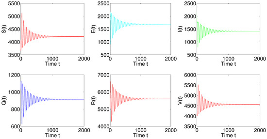
Figure 1.
Time plots of S, E, I, Q, R and V with .
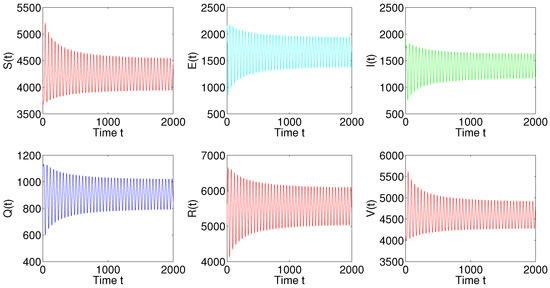
Figure 2.
Time plots of S, E, I, Q, R and V with .

Figure 3.
Bifurcation diagram with respect to time delay of system (22): (a) , (b) , (c) , (d) , (e) , (f) .
(i) Effect of and : In Figure 4, we can see that the number of infectious nodes decreases when the values of and increase. And the system changes its behavior from limit cycle to stable focus as we increase the value of and , which can be shown as in Figure 5.

Figure 4.
Time plots of I for different and at .
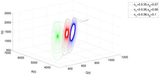
Figure 5.
Dynamic behavior of system (22): projection on I-Q-R for different and at .
(ii) Effect of and : In the same manner, we can see from Figure 6 and Figure 7 that the number of infectious nodes increases when the values of and increase. Also, we observe that system changes its behavior from stale focus to limit cycle as we increase the value of and .

Figure 6.
Time plots of I for different and at .
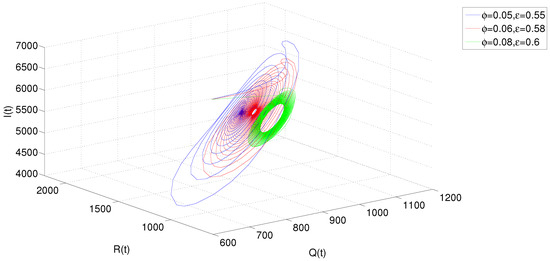
Figure 7.
Dynamic behavior of system (22): projection on I-Q-R for different and at .
(iii) Effect of r and L: As is shown in Figure 8 and Figure 9, the number of infectious nodes increases when the value of r increases and the value of L decreases. In other words, as the density of sensor node increases, the number of infectious nodes increases. In addition, r and L effect the dynamic behavior of system (22) when their value changes. That is, system changes its behavior from stable focus to limit cycle as we increase the value of r and decrease the value of L.

Figure 8.
Time plots of I for different and at .

Figure 9.
Dynamic behavior of system (22): projection on I-Q-R for different and at .
In addition, in the presence of delay, the Lyapunov exponents (LE) have been derived numerically. For a non zero value of , LE for different species have been plotted in Figure 10. As all LEs are negative, then the system is stable.
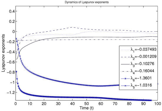
Figure 10.
Other parameters are as in the text.
6. Discussion and Conclusions
In this paper, we present a delayed SEIQRS-V epidemic model for propagation of malicious codes in wireless sensor network based on the work in [32] by incorporating the latent period delay of malicious codes. As stated in [41], one of the significant features of malicious codes is their latent characteristics, which implies that the nodes are infected at time and they are surviving in the latent period and then become infective at time t. In addition, too large time delay may lead to large number of infected nodes, because of which malicious codes propagation persists in the system. Therefore, compared with the model proposed in [33], the delayed model in our paper is more general. It should be also pointed out that there are some proposed epidemic models for propagation of malicious code in a wireless sensor network such as the models in [5,6,9,42,43], but the authors did not consider the characteristics of networks like communication radius and distributed density of nodes in wireless sensor network.
We first find a feasible region which is invariant and where the solutions of our model are positive and the Lyapunov exponent stability is analyzed by constructing a Lyapunov functional. Then, the critical value of time delay at which a Hopf bifurcation occurs is obtained by choosing the delay as the bifurcating parameter. It is found that when the time delay is suitably small (), system (2) is locally asymptotically stable. In this case, the propagation of malicious codes can be controlled easily. However, once the value of the time delay passes through the critical value , system (2) loses its stability and a family of periodic solutions bifurcate from the endemic equilibrium of system (2). In this case, the propagation of malicious codes will be out of control.
Also, the effects of some crucial parameters on dynamics of system (2) are studied by numerical simulations. As the values of and increase, the number of infectious nodes decreases and system (22) changes its behavior from limit cycle to stable focus as we increase the value of and , it is strongly recommended that users of the wireless sensor network should periodically run antivirus software of the newest version, so that the propagation of malicious codes can be controlled. This phenomenon can also be illustrated by the effects of and on dynamics of the system. In addition, the number of infectious nodes increases when the density of the sensor node increases. Thus, it can be concluded that the manager of the wireless sensor network should control the number of nodes connected to the network properly.
Author Contributions
All authors have equally contributed to this paper. They have read and approved the final version of the manuscript.
Funding
This research was supported by National Natural Science Foundation of China(Nos.11461024, 61773181), Natural Science Foundation of Inner Mongolia Autonomous Region (No.2018MS01023), Project of Support Program for Excellent Youth Talent in Colleges and Universities of Anhui Province (Nos.gxyqZD2018044, gxbjZD49), Bengbu University National Research Fund Cultivation Project (2017GJPY03).
Conflicts of Interest
The authors declare no conflict of interest.
Appendix A
Appendix B
Appendix C
References
- Keshri, A.K.; Mishra, B.K.; Mallick, D.K. Library formation of known malicious attacks and their future variants. Int. J. Adv. Sci. Technol. 2016, 94, 1–12. [Google Scholar] [CrossRef]
- Singh, J.; Kumar, D.; Hammouch, Z.; Atangana, A. A fractional epidemiological model for computer viruses pertaining to a new fractional derivative. Appl. Math. Comput. 2018, 316, 504–515. [Google Scholar] [CrossRef]
- Keshri, A.K.; Mishra, B.K.; Mallick, D.K. A predator-prey model on the attacking behavior of malicious objects in wireless nanosensor networks. Nano Commun. Netw. 2018, 15, 1–16. [Google Scholar] [CrossRef]
- Cybercrime-Report. Available online: http://cyberseurityventures.com/2015-wp/wp-content/uploads/2017/10/2017-Cybercrime-Report.pdf (accessed on 23 April 2019).
- Khanh, N.H. Dynamics of a worm propagation model with quarantine in wireless sensor networks. Appl. Math. Inf. Sci. 2016, 10, 1739–1746. [Google Scholar] [CrossRef]
- Mishra, B.K.; Kershi, N. Mathematical model on the transmission of worms in wireless sensor network. Appl. Math. Model. 2013, 3, 4103–4111. [Google Scholar] [CrossRef]
- Mishra, B.K.; Pandey, S.K. Dynamic model of worms with vertical transmission in computer network. Appl. Math. Comput. 2011, 217, 8438–8446. [Google Scholar] [CrossRef]
- Xiao, X.; Fu, P.; Dou, C.S.; Li, Q.; Hu, G.W.; Xia, S.T. Design and analysis of SEIQR worm propagation model in mobile internet. Commun. Nonlinear Sci. Numer. Simul. 2017, 43, 341–350. [Google Scholar] [CrossRef]
- Keshri, N.; Mishra, B.K. Stability analysis of a predator-prey model in wireless sensor network. Int. J. Comput. Math. 2014, 91, 928–943. [Google Scholar]
- Yang, L.X.; Yang, X.F. The spread of computer viruses under the influence of removable storage devices. Appl. Math. Comput. 2012, 219, 3914–3922. [Google Scholar] [CrossRef]
- Muroya, Y.; Li, H.X.; Kuziya, T. On global stabiity of a nonresident computer virus model. Acta Math. Sci. 2014, 34B, 1427–1445. [Google Scholar] [CrossRef]
- Wang, F.W.; Zhang, Y.K.; Wang, C.G.; Ma, J.F. Stability analysis of an e-SEIAR model with point-to-group worm propagation. Commun. Nonlinear Sci. Numer. Simul. 2015, 20, 897–904. [Google Scholar] [CrossRef]
- Tang, C.Q.; Wu, Y.H. Global exponential stability of nonresident computer virus models. Nonlinear Anal. Real World Appl. 2017, 34, 149–158. [Google Scholar] [CrossRef]
- Fatima, U.; Ali, M.; Ahmed, N.; Rafiq, M. Numerical modeling of susceptible latent breaking-out quarantine computer virus epidemic dynamics. Heliyon 2018, 4, e00631. [Google Scholar] [CrossRef]
- Zhang, X.X.; Li, C.D. A novel computer virus model with generic nonlinear burst rate. In Proceedings of the International Workshop on Complex Systems and Networks, Doha, Qatar, 8–10 December 2017; pp. 325–329. [Google Scholar]
- Yang, X.F.; Liu, B.; Gan, C.Q. Global stability of an epidemic model of computer virus. Abstr. Appl. Anal. 2014, 2014, 456320. [Google Scholar] [CrossRef]
- Chen, L.J.; Hattaf, K.; Sun, J.T. Optimal control of a delayed SLBS computer virus model. Phys. Stat. Mech. Its Appl. 2015, 427, 244–250. [Google Scholar] [CrossRef]
- Muroya, Y.; Kuniya, T. Global stability of nonresident computer virus models. Math. Methods Appl. Sci. 2015, 38, 281–295. [Google Scholar] [CrossRef]
- Zhou, H.X.; Guo, W. A stochastic worm model. Telecommun. Syst. 2017, 64, 135–145. [Google Scholar] [CrossRef]
- Amador, J. The stochastic SIRA model for computer viruses. Appl. Math. Comput. 2014, 232, 1112–1124. [Google Scholar] [CrossRef]
- Tafazzoli, T.; Sadeghiyan, B.A. Stochastic model for the size of worm origin. Secur. Commun. Netw. 2016, 9, 1103–1118. [Google Scholar] [CrossRef]
- Jafarabadi, A.; Azgomi, M.A. A stochastic epidemiological model for the propagation of active worms considering the dynamicity of network topology. Peer-to-Peer Netw. Appl. 2015, 8, 1008–1022. [Google Scholar] [CrossRef]
- Zhang, C.M.; Zhao, Y.; Wu, Y.J.; Deng, S.W. A stochastic dynamic model of computer viruses. Discret. Dyn. Nat. Soc. 2012, 2012, 264874. [Google Scholar] [CrossRef]
- Keshri, N.; Gupta, A.; Mishra, B.K. Impact of reduced scale free network on wireless sensor network. Phys. Stat. Mech. Its Appl. 2016, 463, 236–245. [Google Scholar] [CrossRef]
- Hosseini, S.; Azgomi, M.A.; Rahmani, A.T. Malware propagation modeling considering software diversity andimmunization. J. Comput. Sci. 2016, 13, 49–67. [Google Scholar] [CrossRef]
- Zhang, C.M.; Huang, H.T. Optimal control strategy for a novel computer virus propagation model on scale-free networks. Phys. Stat. Mech. Its Appl. 2016, 451, 251–265. [Google Scholar] [CrossRef]
- Feng, L.P.; Song, L.P.; Zhao, Q.S.; Wang, H.B. Modeling and stability analysis of worm propagation in wireless sensor network. Math. Probl. Eng. 2015, 2015, 129598. [Google Scholar] [CrossRef]
- Srivastava, A.P.; Awasthi, S.; Ojha, R.P.; Srivastava, P.K.; Katiyar, S. Stability analysis of SIDR model for worm propagation in wireless sensor network. Indian J. Sci. Technol. 2016, 9, 1–5. [Google Scholar] [CrossRef]
- Nwokoye, C.H.; Ejiofor, W.E.; Orji, R. Investigating the effect of uniform random distribution of nodes in wireless sensor networks usingan epidemic worm model. In Proceedings of the CORI’16, Ibadan, Nigeria, 7–9 September 2016; pp. 58–63. [Google Scholar]
- Singh, A.; Awasthi, A.K.; Singh, K.; Srivastava, P.K. Modeling and analysis of worm propagation in wireless sensor networks. Wirel. Pers. Commun. 2018, 98, 2535–2551. [Google Scholar] [CrossRef]
- Ojha, R.P.; Sanyal, G.; Srivastava, P.K.; Sharma, K. Design and analysis of modified SIQRS model for performance study of wireless sensor network. Scalable Comput. 2017, 18, 229–241. [Google Scholar] [CrossRef]
- Mishra, B.K.; Tyagi, I. Defending against malicious threats in wireless sensor network: A mathematical model. Int. J. Inf. Technol. Comput. Sci. 2014, 6, 12–19. [Google Scholar] [CrossRef]
- Nwokoye, C.H.; Umeh, I.I. The SEIQR-V Model: On a More Accurate Analytical Characterization of Malicious Threat Defense. Int. J. Inf. Technol. Comput. Sci. 2017, 12, 28–37. [Google Scholar] [CrossRef][Green Version]
- Keshri, N.; Mishra, B.K. Two time-delay dynamic model on the transmission of malicious signals in wireless sensor network. Chaos Solitons Fractals 2014, 68, 151–158. [Google Scholar] [CrossRef]
- Zhang, Z.Z.; Bi, D.J. Bifurcation analysis in a delayed computer virus model with the effect of external computers. Adv. Differ. Equat. 2015, 317, 13. [Google Scholar] [CrossRef]
- Zhao, T.; Bi, D.J. Hopf bifurcation of a computer virus spreading model in the network with limited anti-virus ability. Adv. Differ. Equat. 2017, 183, 16. [Google Scholar] [CrossRef]
- Wang, C.L.; Chai, S.X. Hopf bifurcation of an SEIRS epidemic model with delays and vertical transmission in the network. Adv. Differ. Equat. 2016, 10, 19. [Google Scholar] [CrossRef]
- Dai, Y.X.; Lin, Y.P.; Zhao, H.T.; Khalique, C.M. Global stability and Hopf bifurcation of a delayed computer virus propagation model with saturation incidence rate and temporary immunity. Int. J. Mod. Phys. 2016, 30, 1640009. [Google Scholar] [CrossRef]
- Xia, W.J.; Kundu, S.; Maitra, S. Dynamics of a delayed SEIQ epidemic model. Adv. Differ. Equat. 2018, 336, 21. [Google Scholar] [CrossRef]
- Hassard, B.D.; Kazarinoff, N.D.; Wan, Y.H. Theory and Applications of Hopf Bifurcation; Cambridge University Press: Cambridge, UK, 1981. [Google Scholar]
- Ren, J.G.; Yang, X.F.; Yang, L.X.; Xu, Y.H.; Yang, F.Z. A delayed computer virus propagation model and its dynamics. Chaos Solitons Fractals 2012, 45, 74–79. [Google Scholar] [CrossRef]
- Zhang, Z.Z.; Song, L.M. Dynamics of a delayed worm propagation model with quarantine. Adv. Differ. Equat. 2017, 155, 13. [Google Scholar] [CrossRef][Green Version]
- Upadhyay, R.K.; Kumari, S. Bifurcation analysis of an e-epidemic model in wireless sensor network. Int. J. Comput. Math. 2018, 95, 1775–1805. [Google Scholar] [CrossRef]


© 2019 by the authors. Licensee MDPI, Basel, Switzerland. This article is an open access article distributed under the terms and conditions of the Creative Commons Attribution (CC BY) license (http://creativecommons.org/licenses/by/4.0/).