Area Properties of Strictly Convex Curves

Abstract

We study functions defined in the plane ${\mathbb{E}}^2$ in which level curves are strictly convex, and investigate area properties of regions cut off by chords on the level curves. In this paper we give a partial answer to the question: Which function has level curves whose tangent lines cut off from a level curve segment of constant area? In the results, we give some characterization theorems regarding conic sections.

1. Introduction

The most well-known plane curves are straight lines and circles, which are characterized as the plane curves with constant Frenet curvature. The next most familiar plane curves might be the conic sections: ellipses, hyperbolas and parabolas. They are characterized as plane curves with constant affine curvature ([1], p. 4).

The conic sections have an interesting area property. For example, consider the following two ellipses given by $X_k=g^{-1}\left(k\right)$ and $X_l=g^{-1}\left(l\right)$ with $l>k>0$, where

$$g(x,y)=\frac{x^2}{a^2}+\frac{y^2}{b^2},a,b>0.$$

For a fixed point p on $X_k$, we denote by A and B the points where the tangent to $X_k$ at p meets $X_l$. Then the region D bounded by the ellipse $X_l$ and the chord $AB$ outside $X_k$ has constant area independent of the point $p\in X_k$.

In order to give a proof, consider a transformation T of the plane ${\mathbb{E}}^2$ defined by

$$T=\left(\begin{array}{cc}b/\sqrt{ab}& 0\\ 0& a/\sqrt{ab}\end{array}\right).$$

Then $X_k$ and $X_l$ are transformed to concentric circles of radius $\sqrt{abk}$ and $\sqrt{abl}$, respectively; the tangent at p to the tangent at the corresponding point $p^{\prime }$. Since the transformation T is equiaffine (that is, area preserving), a well-known property of concentric circles completes the proof.

For parabolas and hyperbolas given by $g(x,y)=y^2-4ax,a\ne 0$ and $g(x,y)=x^2/a^2-y^2/b^2,a,b>0$, respectively, it is straightforward to show that they also satisfy the above mentioned area properties. For a proof using 1-parameter group of equiaffine transformations, see [1], pp. 6–7.

Conversely, it is reasonable to ask the following question.

Question. Are there any other level curves of a function $g:{\mathbb{R}}^2\to \mathbb{R}$ satisfying the above mentioned area property?

A plane curve X in the plane ${\mathbb{E}}^2$ is called ‘convex’ if it bounds a convex domain in the plane ${\mathbb{E}}^2$ [2]. A convex curve in the plane ${\mathbb{E}}^2$ is called ‘strictly convex’ if the curve has positive Frenet curvature $\kappa$ with respect to the unit normal N pointing to the convex side. We also say that a convex function $f:\mathbb{R}\to \mathbb{R}$ is ‘strictly convex’ if the graph of f is strictly convex.

Consider a smooth function $g:{\mathbb{R}}^2\to \mathbb{R}$. We let $R_g$ denote the set of all regular values of the function g. We suppose that there exists an interval $S_g\subset R_g$ such that for every $k\in S_g$, the level curve $X_k=g^{-1}\left(k\right)$ is a smooth strictly convex curve in the plane ${\mathbb{E}}^2$. We let $S_g$ denote the maximal interval in $R_g$ with the above property. If $k\in S_g$, then there exists a maximal interval $I_k\subset S_g$ such that each $X_{k+h}$ with $k+h\in I_k$ lies in the convex side of $X_k$. The maximal interval $I_k$ is of the form $(k,a)$ or $(b,k)$ according to whether the gradient vector $\nabla g$ points to the convex side of $X_k$ or not.

As examples, consider the two functions $g_i:{\mathbb{R}}^2\to \mathbb{R},i=1,2$ defined by $g_i(x,y)=y^2+{ϵ}_i{a}^2{x}^2$ with positive constant a, ${ϵ}_i={(-1)}^i$. Then, for the function $g_1$ we have $R_{g_1}=\mathbb{R}-\left\{0\right\}$, $S_{g_1}=(0,\infty )$ or $(-\infty ,0)$, $I_k=(k,\infty )$ if $k>0$, and $I_k=(-\infty ,k)$ if $k<0$. For $g_2$, we get $R_{g_2}=S_{g_2}=(0,\infty )$ and $I_k=(0,k)$ with $k\in S_{g_2}$.

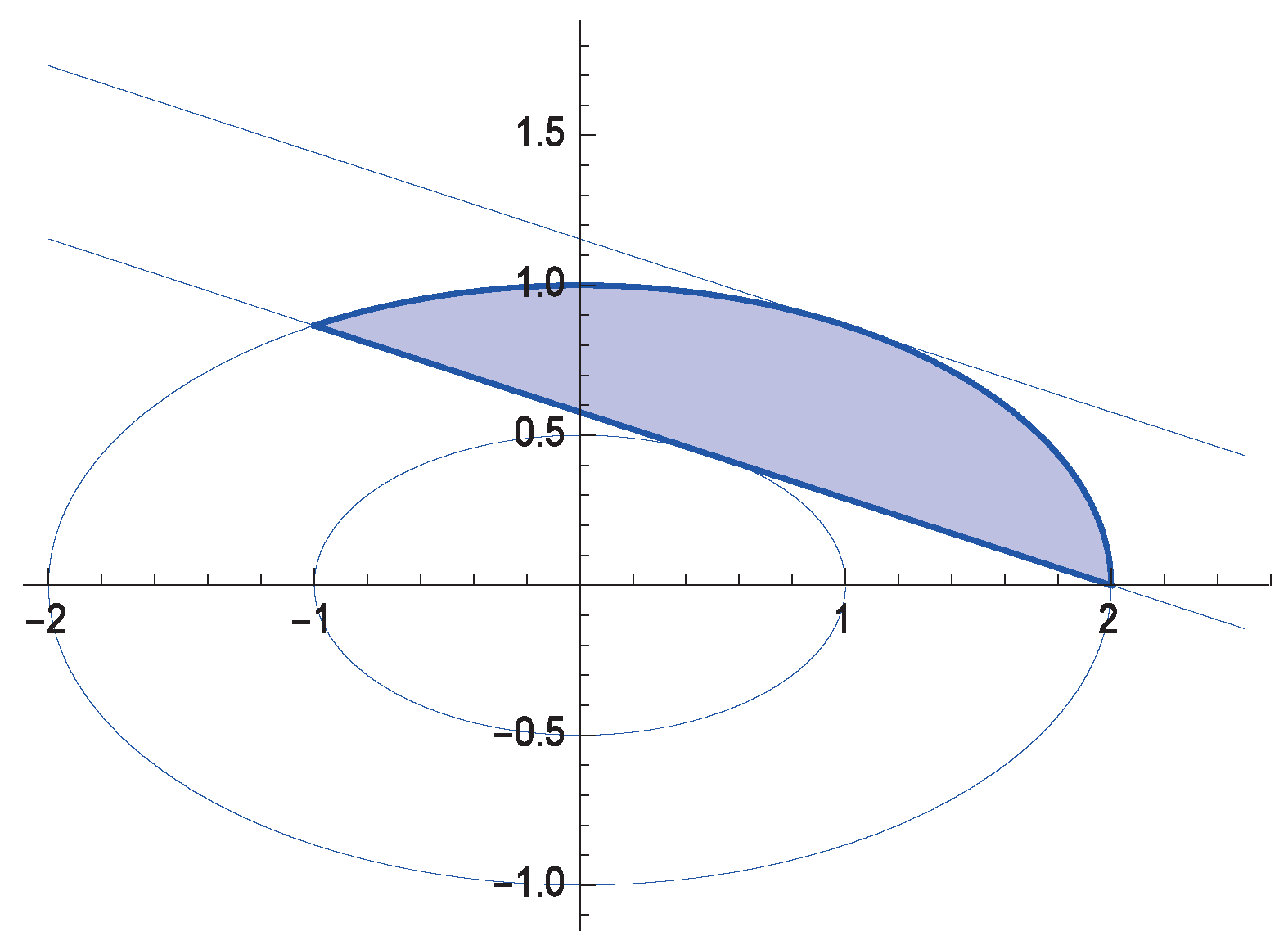
For a fixed point $p\in X_k$ with $k\in S_g$ and a small h with $k+h\in I_k$, we consider the tangent line t to $X_k$ at $p\in X_k$ and the closest tangent line ℓ to $X_{k+h}$ at a point $v\in X_{k+h}$, which is parallel to the tangent line t. We let ${\mathcal{A}}_p^{\ast }(k,h)$ denote the area of the region bounded by $X_k$ and the line ℓ (See Figure 1).

In [3], the following characterization theorem for parabolas was established.

Proposition 1.

We consider a strictly convex function $f:\mathbb{R}\to \mathbb{R}$ and the function $g:{\mathbb{R}}^2\to \mathbb{R}$ given by $g(x,y)=y-f\left(x\right)$. Then, the following conditions are equivalent.

1.

For a fixed $k\in \mathbb{R}$, ${\mathcal{A}}_p^{\ast }(k,h)$ is a function ${\varphi }_k\left(h\right)$ of only h.

2.

Up to translations, the function $f\left(x\right)$ is a quadratic polynomial given by $f\left(x\right)=a{x}^2$ with $a>0$, and hence every level curve $X_k$ of g is a parabola.

In the above proposition, we have $R_g=S_g=\mathbb{R}$ and $I_k=(k,\infty )$.

In particular, Archimedes proved that every level curve $X_k$ (parabola) of the function $g(x,y)=y-a{x}^2$ in the Euclidean plane ${\mathbb{E}}^2$ satisfies ${\mathcal{A}}_p^{\ast }(k,h)=ch\sqrt{h}$ for some constant c which depends only on the parabola [4].

In this paper, we investigate the family of strictly convex level curves $X_k,k\in S_g$ of a function $g:{\mathbb{R}}^2\to \mathbb{R}$ which satisfies the following condition.

$\left({\mathcal{A}}^{\ast }\right)$: For $k\in S_g$ with $k+h\in I_k$, ${\mathcal{A}}_p^{\ast }(k,h)$ with $p\in X_k$ is a function ${\varphi }_k\left(h\right)$ of only k and h.

In order to investigate the family of strictly convex level curves $X_k,k\in S_g$ of a function $g:{\mathbb{R}}^2\to \mathbb{R}$ satisfying condition $\left({\mathcal{A}}^{\ast }\right)$, first of all, in Section 2 we introduce a useful lemma which reveals a relation between the curvature of level curves and the gradient of the function g (Lemma 3 in Section 2).

Next, using Lemma 3, in Section 3 we establish the following characterizations for conic sections.

Theorem 1.

Let $f:\mathbb{R}\to \mathbb{R}$ be a smooth function. We let g denote the function defined by $g(x,y)=y^a-f\left(x\right)$, where a is a nonzero real number with $a\ne 1$. Suppose that the level curves $X_k(k\in S_g)$ of g in the plane ${\mathbb{E}}^2$ are strictly convex. Then the following conditions are equivalent.

1.

The function g satisfies $\left({\mathcal{A}}^{\ast }\right)$.

2.

For $k\in S_g$, ${\kappa \left(p\right)|\nabla g\left(p\right)|}^3=c\left(k\right)$ is constant on $X_k$, where $\kappa \left(p\right)$ denotes the curvature of $X_k$ at $p\in X_k$.

3.

We have $a=2$ and the function f is a quadratic function. Hence, each $X_k$ is a conic section.

In case the function f ($-f$, resp.) is itself a non-negative strictly convex function, Theorem 1 is a special case ($n=1$) of Theorem 2 (Theorem 3, resp.) in [5].

In Section 4 we prove the following.

Theorem 2.

Let $f:\mathbb{R}\to \mathbb{R}$ be a smooth function. For a rational function $j\left(y\right)$ in y, we let g denote the function defined by $g(x,y)=f\left(x\right)+j\left(y\right)$. Suppose that the level curves $X_k(k\in S_g)$ of g in the plane ${\mathbb{E}}^2$ are strictly convex. Then the following conditions are equivalent.

1.

The function g satisfies $\left({\mathcal{A}}^{\ast }\right)$.

2.

For $k\in S_g$, ${\kappa \left(p\right)|\nabla g\left(p\right)|}^3=c\left(k\right)$ is constant on $X_k$, where $\kappa \left(p\right)$ denotes the curvature of $X_k$ at $p\in X_k$.

3.

Both of the functions $j\left(y\right)$ and $f\left(x\right)$ are quadratic. Hence, each $X_k$ is a conic section.

When the function g is homogeneous, in Section 5 we prove the following characterization theorem for conic sections.

Theorem 3.

Let $g:{\mathbb{R}}^2\to \mathbb{R}$ be a smooth homogeneous function of degree d. Suppose that the level curves $X_k$ of g with $k\in S_g$ in the plane ${\mathbb{E}}^2$ are strictly convex. Then the following conditions are equivalent.

1.

The function g satisfies $\left({\mathcal{A}}^{\ast }\right)$.

2.

For $k\in S_g$, ${\kappa \left(p\right)|\nabla g\left(p\right)|}^3=c\left(k\right)$ is constant on $X_k$, where $\kappa \left(p\right)$ denotes the curvature of $X_k$ at $p\in X_k$.

3.

The function g is given by

$$g(x,y)={(a{x}^2+2hxy+b{y}^2)}^{d/2},$$

where $a,b$ and h satisfy $ab-h^2\ne 0$. Thus, each $X_k$ is either a hyperbola or an ellipse centered at the origin.

Finally, we prove the following in Section 6.

Proposition 2.

There exists a function $g(x,y)=f\left(x\right)+j\left(y\right)$ which satisfies the following.

1.

Every level curve of g is strictly convex with $S_g=\mathbb{R}$.

2.

For $k\in S_g$, ${\kappa \left(p\right)|\nabla g\left(p\right)|}^3=c\left(k\right)$ is constant on $X_k$, where $\kappa \left(p\right)$ denotes the curvature of $X_k$ at $p\in X_k$.

3.

The function g does not satisfy $\left({\mathcal{A}}^{\ast }\right)$.

A lot of properties of conic sections (especially, parabolas) have been proved to be characteristic ones [6,7,8,9,10,11,12,13]. For hyperbolas and ellipses centered at the origin, using the support function h and the curvature function $\kappa$ of a plane curve, a characterization theorem was established [14], from which we get the proof of Theorem 3 in Section 5.

Some characterization theorems for hyperplanes, circular hypercylinders, hyperspheres, elliptic paraboloids and elliptic hyperboloids in the Euclidean space ${\mathbb{E}}^{n+1}$ were established in [5,15,16,17,18,19]. For a characterization of hyperbolic space in the Minkowski space ${\mathbb{E}}_1^{n+1}$, we refer to [20].

In this article, all functions are smooth ($C^{\left(3\right)}$).

2. Preliminaries

Suppose that X is a smooth strictly convex curve in the plane ${\mathbb{E}}^2$ with the unit normal N pointing to the convex side. For a fixed point $p\in X$ and for a sufficiently small $h>0$, we take the line ℓ passing through the point $p+hN\left(p\right)$ which is parallel to the tangent t to X at p. We denote by A and B the points where the line ℓ meets the curve X and put ${\mathcal{L}}_p\left(h\right)$ and ${\mathcal{A}}_p\left(h\right)$ the length of the chord $AB$ of X and the area of the region bounded by the curve and the line ℓ, respectively.

Without loss of generality, we may take a coordinate system $(x,y)$ of ${\mathbb{E}}^2$ with the origin p, the tangent line to X at p is the x-axis. Hence X is locally the graph of a strictly convex function $f:\mathbb{R}\to \mathbb{R}$ with $f\left(p\right)=0$.

For a sufficiently small $h>0$, we get

$$\begin{array}{cc}\hfill {\mathcal{A}}_p\left(h\right)& ={\int }_{I_p\left(h\right)}\{h-f\left(x\right)\}dx,\hfill \\ \hfill {\mathcal{L}}_p\left(h\right)& ={\int }_{I_p\left(h\right)}1dx,\hfill \end{array}$$

where we put $I_p\left(h\right)=\{x\in \mathbb{R}|f\left(x\right)<h\}$ and ${\mathcal{L}}_p\left(h\right)$ is nothing but the length of $I_p\left(h\right)$. Note that we also have

$$\begin{array}{c}\hfill {\mathcal{A}}_p\left(h\right)={\int }_{y=0}^h{\mathcal{L}}_p\left(y\right)dy={\int }_{y=0}^h\{{\int }_{I_p\left(y\right)}1dx\}dy,\end{array}$$

from which we obtain

$$\begin{array}{c}\hfill {\mathcal{A}}_p^{\prime }\left(h\right)={\mathcal{L}}_p\left(h\right).\end{array}$$

We have the following [3]:

Lemma 1.

Suppose that X is a smooth strictly convex curve in the plane ${\mathbb{E}}^2$. Then for a point $p\in X$ we have

$$\begin{array}{cc}\hfill \underset{t\to 0}{lim}\frac{1}{\sqrt{t}}{\mathcal{L}}_p\left(t\right)& =\frac{2\sqrt{2}}{\sqrt{\kappa \left(p\right)}}\hfill \end{array}$$

and

$$\begin{array}{cc}\hfill \underset{t\to 0}{lim}\frac{1}{t\sqrt{t}}{\mathcal{A}}_p\left(t\right)& =\frac{4\sqrt{2}}{3\sqrt{\kappa \left(p\right)}},\hfill \end{array}$$

where $\kappa \left(p\right)$ is the curvature of X at p.

Now, we consider the family of strictly convex level curves $X_k=g^{-1}\left(k\right)$ of a function $g:{\mathbb{R}}^2\to \mathbb{R}$ with $k\in S_g$.

Suppose that the function g satisfies condition $\left({\mathcal{A}}^{\ast }\right)$. For each $k\in S_g$ and $p\in X_k$ we denote by $\kappa \left(p\right)$ the curvature of $X_k$ at p

By considering $-g$ if necessary, we may assume that $I_k$ is of the form $(k,a)$ with $k<a$, and hence we have $N=\nabla g/|\nabla g|$ on $X_k$. For a fixed point $p\in X_k$ and a small $t>0$, we have

$$\begin{array}{c}\hfill {\mathcal{A}}_p\left(t\right)={\mathcal{A}}_p^{\ast }(k,h\left(t\right))={\varphi }_k\left(h\left(t\right)\right),\end{array}$$

where $h=h\left(t\right)$ is a function with $h\left(0\right)=0$. Differentiating with respect to t gives

$$\begin{array}{c}\hfill {\mathcal{L}}_p\left(t\right)={\mathcal{A}}_p^{\prime }\left(t\right)={\varphi }_k^{\prime }\left(h\right)h^{\prime }\left(t\right),\end{array}$$

where ${\varphi }_k^{\prime }\left(h\right)$ is the derivative of ${\varphi }_k$ with respect to h. This shows that

$$\begin{array}{c}\hfill \frac{1}{\sqrt{t}}{\mathcal{L}}_p\left(t\right)=\frac{{\varphi }_k^{\prime }\left(h\right)}{\sqrt{h}}\sqrt{\frac{h\left(t\right)}{t}}{h}^{\prime }\left(t\right).\end{array}$$

(1)

Next, we use the following lemma for the limit of $h^{\prime }\left(t\right)$ as $t\to 0$.

Lemma 2.

We have

$$\begin{array}{c}\hfill \underset{t\to 0}{lim}{h}^{\prime }\left(t\right)=|\nabla g\left(p\right)|.\end{array}$$

(2)

Proof. 

See the proof of Lemma 8 in [5].  □

It follows from (2) that

$$\begin{array}{c}\hfill \underset{t\to 0}{lim}\sqrt{\frac{h\left(t\right)}{t}}=\sqrt{|\nabla g(p\left)\right|}.\end{array}$$

(3)

Together with Lemma 1, (2) and (3), (1) implies that ${lim}_{h\to 0}{\varphi }_k^{\prime }\left(h\right)/\sqrt{h}$ exists (say, $\gamma \left(k\right)$), which is independent of $p\in X_k$. Furthermore, we also obtain

$$\begin{array}{c}\hfill {\kappa \left(p\right)|\nabla g\left(p\right)|}^3=\frac{8}{\gamma {\left(k\right)}^2},\end{array}$$

which is constant on the level curve $X_k$.

Finally, we obtain the following lemma which is useful in the proof of Theorems stated in Section 1.

Lemma 3.

We suppose that a function $g:{\mathbb{R}}^2\to \mathbb{R}$ satisfies condition $\left({\mathcal{A}}^{\ast }\right)$. Then, for each $k\in S_g$, on $X_k$ the function defined by

$$\begin{array}{c}\hfill {\kappa \left(p\right)|\nabla g\left(p\right)|}^3=c\left(k\right)\end{array}$$

is constant on $X_k$, where $\kappa \left(p\right)$ is the curvature of $X_k$ at p.

Remark 1.

Lemma 3 is a special case ($n=1$) of Lemma 8 in [5]. For conveniences, we gave a brief proof.

3. Proof of Theorem 1

In this section, we give a proof of Theorem 1 stated in Section 1.

For a nonzero real number $a(\ne 1)$ and a smooth function $f:\mathbb{R}\to \mathbb{R}$, we investigate the level curves of the function $g=g_a:{\mathbb{R}}^2\to \mathbb{R}$ defined by $g_a(x,y)=y^a-f\left(x\right)$.

Suppose that the function g satisfies condition $\left({\mathcal{A}}^{\ast }\right)$. Then, it follows from Lemma 3 that on the level curve $X_k=g^{-1}\left(k\right)$ with $k\in S_g$ we have

$$\begin{array}{c}\hfill {\kappa \left(p\right)|\nabla g\left(p\right)|}^3=c\left(k\right),\end{array}$$

(4)

where $c\left(k\right)$ is a function of $k\in S_g$.

Note that for $p=(x,y)\in X_k$ with $y^a=f\left(x\right)+k$ we have

$$\begin{array}{c}\hfill {|\nabla g\left(p\right)|}^3={\{f^{\prime }{\left(x\right)}^2+a^2{(f\left(x\right)+k)}^{\frac{2a-2}{a}}\}}^{\frac{3}{2}},\end{array}$$

and hence

$$\begin{array}{c}\hfill {\kappa \left(p\right)|\nabla g\left(p\right)|}^3=|a^2{(f\left(x\right)+k)}^{\frac{2a-2}{a}}{f}^{″}\left(x\right)+a(1-a){(f\left(x\right)+k)}^{\frac{a-2}{a}}{f}^{\prime }{\left(x\right)}^2|.\end{array}$$

(5)

Thus, it follows from (4) and (5) that for some nonzero $c=c\left(k\right)$ with $k\in S_g$, the function $f\left(x\right)$ satisfies

$$\begin{array}{c}\hfill a^2{(f\left(x\right)+k)}^{\frac{2a-2}{a}}{f}^{″}\left(x\right)+a(1-a){(f\left(x\right)+k)}^{\frac{a-2}{a}}{f}^{\prime }{\left(x\right)}^2=c\left(k\right),\end{array}$$

which can be rewritten as

$$\begin{array}{c}\hfill f^{″}\left(x\right)+\frac{1-a}{a}{(f\left(x\right)+k)}^{-1}{f}^{\prime }{\left(x\right)}^2=\frac{c\left(k\right)}{a^2}{(f\left(x\right)+k)}^{\frac{2-2a}{a}}.\end{array}$$

(6)

By differentiating (6) with respect to k, we get

$$\begin{array}{c}\hfill f^{\prime }{\left(x\right)}^2=\frac{c^{\prime }\left(k\right)}{a(a-1)}{(f\left(x\right)+k)}^{\frac{2}{a}}-2\frac{c\left(k\right)}{a^2}{(f\left(x\right)+k)}^{\frac{2-a}{a}}.\end{array}$$

(7)

Putting $u=f\left(x\right)+k$ and $v=du/dx=f^{\prime }\left(x\right)$, we get from (6)

$$\begin{array}{c}\hfill \frac{dv}{du}+\frac{1-a}{a}{u}^{-1}v=\frac{c\left(k\right)}{a^2}{u}^{\frac{2-2a}{a}}{v}^{-1},\end{array}$$

(8)

which is a Bernoulli equation. By letting $w=v^2$, we obtain

$$\begin{array}{c}\hfill \frac{dw}{du}+\frac{2-2a}{a}{u}^{-1}w=\frac{2c\left(k\right)}{a^2}{u}^{\frac{2-2a}{a}}.\end{array}$$

(9)

Since $u^{\frac{2-2a}{a}}$ is an integrating factor of (9), we get

$$\begin{array}{c}\hfill \frac{d}{du}(w{u}^{\frac{2-2a}{a}})=\frac{2c\left(k\right)}{a^2}{u}^{\frac{4-4a}{a}}.\end{array}$$

(10)

Now, in order to integrate (10), we divide by some cases as follows.

Case 1. Suppose that $a=\frac{4}{3}$. Then, from (10) we have

$$\begin{array}{c}\hfill w=\{\frac{9c\left(k\right)}{8}lnu+b\left(k\right)\}\sqrt{u},\end{array}$$

(11)

where $b=b\left(k\right)$ is a constant. Since $u=f\left(x\right)+k$ and $w=f^{\prime }{\left(x\right)}^2$, (7) and (11) show that

$$\begin{array}{c}\hfill c\left(k\right)ln(f\left(x\right)+k)+\frac{8}{9}b\left(k\right)=2c^{\prime }\left(k\right)(f\left(x\right)+k)-c\left(k\right).\end{array}$$

(12)

By differentiating (12) with respect to x, we obtain

$$\begin{array}{c}\hfill 2c^{\prime }\left(k\right)(f\left(x\right)+k)=c\left(k\right).\end{array}$$

(13)

Since $c\left(k\right)$ is nonzero, (13) leads to a contradiction.

Case 2. Suppose that $a\ne \frac{4}{3}$. Then, from (8) we have

$$\begin{array}{c}\hfill w=a\left(k\right)u^{\alpha }+b\left(k\right)u^{\beta },a\left(k\right)=\frac{2c\left(k\right)}{(4-3a)a},\alpha =\frac{2-a}{a},\beta =\frac{2a-2}{a},\end{array}$$

(14)

where $b=b\left(k\right)$ is a constant. Since $u=f\left(x\right)+k$ and $w=f^{\prime }{\left(x\right)}^2$, it follows from (7) and (14) that

$$\begin{array}{c}\hfill b\left(k\right){(f\left(x\right)+k)}^{\frac{3a-4}{a}}=\frac{c^{\prime }\left(k\right)}{a(a-1)}(f\left(x\right)+k)-4c\left(k\right)\frac{a-2}{a^2(3a-4)}.\end{array}$$

(15)

By differentiating (15) with respect to x, we get

$$\begin{array}{c}\hfill b\left(k\right){(f\left(x\right)+k)}^{\frac{2a-4}{a}}=\frac{c^{\prime }\left(k\right)}{a(a-1)}.\end{array}$$

(16)

If $b\left(k\right)\ne 0$, then (16) shows that $a=2$. If $b\left(k\right)=0$, then it follows from (15) and (16) that $c^{\prime }\left(k\right)=0$, and hence $a=2$.

Finally, we consider the remaining case as follows.

Case 3. Suppose that $a=2$. Then, it follows from (7) that for the constant $c=c\left(k\right)$

$$\begin{array}{c}\hfill f^{\prime }{\left(x\right)}^2=\frac{c^{\prime }\left(k\right)}{2}(f\left(x\right)+k)-\frac{c\left(k\right)}{2}.\end{array}$$

(17)

If $c^{\prime }\left(k\right)=0$, that is, c is independent of k, then (17) shows that $f\left(x\right)$ is a linear function. Hence each level curve $X_k$ of the function $g(x,y)=y^2-f\left(x\right)$ is a parabola. If $c^{\prime }\left(k\right)\ne 0$, then differentiating both sides of (17) with respect to x shows

$$\begin{array}{c}\hfill 4f^{″}\left(x\right)=c^{\prime }\left(k\right).\end{array}$$

This yields that $f\left(x\right)$ is a quadratic function and $c\left(k\right)$ is a linear function in k.

Combining Cases 1–3, we proved the following:

$$\begin{array}{c}\hfill 1)\Rightarrow 2)\Rightarrow 3).\end{array}$$

Conversely, suppose that the function g is given by

$$g(x,y)=y^2-(a{x}^2+bx+c),$$

where $a,b$ and c are constants with $a^2+b^2\ne 0$. Then, each level curve $X_k$ of g is an ellipse ($a<0$), a hyperbola ($a>0$) or a parabola ($a=0,b\ne 0$). It follows from Section 1 or [4], pp. 6–7 that the function g satisfies condition $\left({\mathcal{A}}^{\ast }\right)$.

This shows that Theorem 1 holds.

Remark 2.

It follows from the proof of Theorem 1 that the constant $c=c\left(k\right)$ is independent of k if $g(x,y)=y^2-4ax,a\ne 0$ and it is a linear function in k if $g(x,y)=y^2-a{x}^2,a\ne 0$.

Finally, we note the following.

Remark 3.

Suppose that a smooth function $g:{\mathbb{R}}^2\to \mathbb{R}$ satisfies condition $\left({\mathcal{A}}^{\ast }\right)$ with

$$\begin{array}{c}\hfill {\kappa \left(p\right)|\nabla g\left(p\right)|}^3=c\left(k\right),\end{array}$$

where $p\in X_k=g^{-1}\left(k\right)$ and $k\in S_g$. Then for any positive constant d, there exists a composite function $G=\varphi \circ g$ satisfying condition $\left({\mathcal{A}}^{\ast }\right)$ with

$$\begin{array}{c}\hfill {\kappa \left(p\right)|\nabla G\left(p\right)|}^3=d.\end{array}$$

(18)

Note that the function $G=\varphi \circ g$ has the same level curves as the function g.

In order to prove (18), we denote by $\varphi \left(t\right)$ an indefinite integral of the function ${(d/c\left(t\right))}^{1/3}$. Then for $p\in G^{-1}\left(k\right)=g^{-1}\left({\varphi }^{-1}\left(k\right)\right)$ we get

$$\begin{array}{c}\hfill |\nabla G\left(p\right)|={\varphi }^{\prime }\left(g\left(p\right)\right)|\nabla g\left(p\right)|.\end{array}$$

Hence, on each level curve $G^{-1}\left(k\right)=g^{-1}\left({\varphi }^{-1}\left(k\right)\right)$ we obtain

$$\begin{array}{c}\hfill {\kappa \left(p\right)|\nabla G\left(p\right)|}^3=c\left({\varphi }^{-1}\left(k\right)\right){\varphi }^{\prime }{\left({\varphi }^{-1}\left(k\right)\right)}^3=d.\end{array}$$

4. Proof of Theorem 2

In this section, we give a proof of Theorem 2.

We consider a function g defined by $g(x,y)=f\left(x\right)+j\left(y\right)$ for some functions $f\left(x\right)$ and $j\left(y\right)$. Then at the point $p\in X_k=g^{-1}\left(k\right)$ we have

$$\begin{array}{cc}\hfill {|\nabla g\left(p\right)|}^3& ={\{f^{\prime }{\left(x\right)}^2+j^{\prime }{\left(y\right)}^2\}}^{\frac{3}{2}},\hfill \\ \hfill {\kappa \left(p\right)|\nabla g\left(p\right)|}^3& =|f^{″}\left(x\right)j^{\prime }{\left(y\right)}^2+f^{\prime }{\left(x\right)}^2{j}^{″}\left(y\right)|.\hfill \end{array}$$

Suppose that the function g satisfies condition $\left({\mathcal{A}}^{\ast }\right)$. Then, it follows from Lemma 3 that on the level curve $X_k:f\left(x\right)+j\left(y\right)=k$ we get for some nonzero constant $c=c\left(k\right)$

$$\begin{array}{c}\hfill f^{″}\left(x\right)j^{\prime }{\left(y\right)}^2+f^{\prime }{\left(x\right)}^2{j}^{″}\left(y\right)=c\left(k\right),\end{array}$$

(19)

which shows that the set $V=\{(x,y)\in X_k|f^{\prime }\left(x\right)=0\mathrm{o}r{j}^{\prime }\left(y\right)=0\}$ has no interior points in the level curve $X_k$. Hence by continuity, without loss of generality we may assume that V is empty.

First, we consider y as a function of x and k. Then, we rewrite (19) as follows

$$\begin{array}{c}\hfill f^{″}\left(x\right)+f^{\prime }{\left(x\right)}^2\frac{j^{″}\left(y\right)}{j^{\prime }{\left(y\right)}^2}=\frac{c\left(k\right)}{j^{\prime }{\left(y\right)}^2},j\left(y\right)+f\left(x\right)=k.\end{array}$$

(20)

Putting $u=-f\left(x\right)+k$ and $v=du/dx=-f^{\prime }\left(x\right)$, we get

$$\begin{array}{c}\hfill \frac{dv}{du}-\frac{j^{″}\left(y\right)}{j^{\prime }{\left(y\right)}^2}v=-\frac{c\left(k\right)}{j^{\prime }{\left(y\right)}^2}{v}^{-1},\end{array}$$

which is a Bernoulli equation. By letting $w=v^2=f^{\prime }{\left(x\right)}^2$, we obtain

$$\begin{array}{c}\hfill \frac{dw}{du}-\frac{2j^{″}\left(y\right)}{j^{\prime }{\left(y\right)}^2}w=-\frac{2c\left(k\right)}{j^{\prime }{\left(y\right)}^2}.\end{array}$$

(21)

Since $u=j\left(y\right)$, we see that $j^{\prime }{\left(y\right)}^{-2}$ is an integrating factor of (21). Hence we get

$$\begin{array}{c}\hfill \frac{d}{du}(w{j}^{\prime }{\left(y\right)}^{-2})=-2c\left(k\right)j^{\prime }{\left(y\right)}^{-4}.\end{array}$$

Thus we obtain

$$\begin{array}{c}\hfill f^{\prime }{\left(x\right)}^2=w=-2c\left(k\right)j^{\prime }{\left(y\right)}^2\{\varphi \left(y\right)+d\left(k\right)\},\end{array}$$

(22)

where $\varphi \left(y\right)$ is a function of y satisfying ${\varphi }^{\prime }\left(y\right)=j^{\prime }{\left(y\right)}^{-3}$ and $d=d\left(k\right)$ is a constant.

On the other hand, by differentiating (20) with respect to k, we get

$$\begin{array}{c}\hfill f^{\prime }{\left(x\right)}^2\{j^{\prime }\left(y\right)j^{‴}\left(y\right)-2j^{″}{\left(y\right)}^2\}=c^{\prime }\left(k\right)j^{\prime }{\left(y\right)}^2-2c\left(k\right)j^{″}\left(y\right).\end{array}$$

(23)

It follows from (22) and (23) that

$$\begin{array}{c}\hfill a\left(k\right)j^{\prime }{\left(y\right)}^2-j^{″}\left(y\right)=j^{\prime }{\left(y\right)}^2\{2j^{″}{\left(y\right)}^2-j^{\prime }\left(y\right)j^{‴}\left(y\right)\}\{\varphi \left(y\right)+d\left(k\right)\},\end{array}$$

(24)

where we use $a\left(k\right)=\frac{c^{\prime }\left(k\right)}{2c\left(k\right)}$. Or equivalently, we get

$$\begin{array}{c}\hfill \varphi \left(y\right)+d\left(k\right)=\frac{a\left(k\right)j^{\prime }{\left(y\right)}^2-j^{″}\left(y\right)}{j^{\prime }{\left(y\right)}^2\{2j^{″}{\left(y\right)}^2-j^{\prime }\left(y\right)j^{‴}\left(y\right)\}},\end{array}$$

(25)

where the denominator does not vanish. Even though $j\left(y\right)$ was assumed to be $C^{\left(3\right)}$, (24) implies that the function $\{2j^{″}{\left(y\right)}^2-j^{\prime }\left(y\right)j^{‴}\left(y\right)\}$ is differentiable. By differentiating (25) with respect to x, it is straightforward to show that

$$\begin{array}{c}\hfill \{a\left(k\right)j^{\prime }{\left(y\right)}^2-j^{″}\left(y\right)\}\frac{d}{dy}\{2j^{″}{\left(y\right)}^2-j^{\prime }\left(y\right)j^{‴}\left(y\right)\}=0.\end{array}$$

(26)

Together with (24), (26) yields that $2j^{″}{\left(y\right)}^2-j^{\prime }\left(y\right)j^{‴}\left(y\right)$ is constant. Hence, for some constant $\alpha$ we have

$$\begin{array}{c}\hfill 2j^{″}{\left(y\right)}^2-j^{\prime }\left(y\right)j^{‴}\left(y\right)=\alpha .\end{array}$$

(27)

Next, interchanging the role of x and y in the above discussions, we consider x as a function of y and k. Then, (22) gives

$$\begin{array}{c}\hfill j^{\prime }{\left(y\right)}^2=-2c\left(k\right)f^{\prime }{\left(x\right)}^2\{\psi \left(x\right)+e\left(k\right)\},\end{array}$$

(28)

where $\psi \left(x\right)$ is a function of x satisfying ${\psi }^{\prime }\left(x\right)=f^{\prime }{\left(x\right)}^{-3}$ and $e=e\left(k\right)$ is a constant. In the same argument as the above, we obtain the corresponding equations from (23)–(27). For example, we get from (26)

$$\begin{array}{c}\hfill \{a\left(k\right)f^{\prime }{\left(x\right)}^2-f^{″}\left(x\right)\}\frac{d}{dx}\{2f^{″}{\left(x\right)}^2-f^{\prime }\left(x\right)f^{‴}\left(x\right)\}=0.\end{array}$$

(29)

Thus, for some constant $\beta$, we also get

$$\begin{array}{c}\hfill 2f^{″}{\left(x\right)}^2-f^{\prime }\left(x\right)f^{‴}\left(x\right)=\beta .\end{array}$$

(30)

By integrating (24) and (30) respectively, we obtain for some constants $\gamma$ and $\delta$

$$\begin{array}{c}\hfill 2j^{″}{\left(y\right)}^2=\gamma j^{\prime }{\left(y\right)}^4+\alpha \end{array}$$

(31)

and its corresponding equation

$$\begin{array}{c}\hfill 2f^{″}{\left(x\right)}^2=\delta f^{\prime }{\left(x\right)}^4+\beta .\end{array}$$

(32)

Differentiating (19) with respect to x, we have

$$\begin{array}{c}\hfill \frac{1}{j^{\prime }\left(y\right)}\{f^{‴}\left(x\right)j^{\prime }{\left(y\right)}^3-f^{\prime }{\left(x\right)}^3{j}^{‴}\left(y\right)\}=\frac{d}{dx}\{f^{″}\left(x\right)j^{\prime }{\left(y\right)}^2+f^{\prime }{\left(x\right)}^2{j}^{″}\left(y\right)\}=0.\end{array}$$

(33)

Together with (31) and (32), this shows that $j\left(y\right)$ is quadratic in y if and only if $f\left(x\right)$ is quadratic in x.

Hereafter, we assume that neither $f\left(x\right)$ nor $j\left(y\right)$ are quadratic. Then, combining (27), (30), (31) and (32), it follows from (33) that

$$\begin{array}{c}\hfill (\gamma -\delta )f^{\prime }{\left(x\right)}^4{j}^{\prime }{\left(y\right)}^4=0,\end{array}$$

which shows that $\gamma =\delta$. Hence, for a nonzero constant $\gamma$ the functions $f\left(x\right)$ and $j\left(y\right)$ satisfy, respectively

$$\begin{array}{c}\hfill 2f^{″}{\left(x\right)}^2=\gamma f^{\prime }{\left(x\right)}^4+\beta \end{array}$$

(34)

and

$$\begin{array}{c}\hfill 2j^{″}{\left(y\right)}^2=\gamma j^{\prime }{\left(y\right)}^4+\alpha .\end{array}$$

(35)

Differentiating (34) and (35) with respect to x and y, respectively, implies

$$\begin{array}{c}\hfill f^{‴}\left(x\right)=\gamma f^{\prime }{\left(x\right)}^3,j^{‴}\left(y\right)=\gamma j^{\prime }{\left(y\right)}^3,\end{array}$$

(36)

where $\gamma$ is a nonzero constant.

Conversely, we prove the following for later use in Section 6.

Lemma 4.

Suppose that the functions $f\left(x\right)$ and $j\left(y\right)$ satisfy (34) and (35) for some constants α and β, respectively. Then on each level curve $X_k$ with $k\in S_g$ of the function $g(x,y)=f\left(x\right)+j\left(y\right)$, ${\kappa \left(p\right)|\nabla g\left(p\right)|}^3$ is constant.

Proof. 

Using (36), it follows from the first equality of (33) that on the level curve $X_k$ of the function g, we have

$$\begin{array}{c}\hfill \frac{d}{dx}\{f^{″}\left(x\right)j^{\prime }{\left(y\right)}^2+f^{\prime }{\left(x\right)}^2{j}^{″}\left(y\right)\}=0.\end{array}$$

This completes the proof of Lemma 4.  □

Finally, we proceed on our way. We divide by two cases as follows.

Case 1. Suppose that $j\left(y\right)$ is a polynomial of degree $degh=n\ge 3$. Then, by counting the degree of both sides of the second equation in (36) we see that the constant $\gamma$ must vanish. This contradiction shows that the polynomial $j\left(y\right)$ is quadratic.

Case 2. Suppose that $j\left(y\right)$ is a rational function given by

$$\begin{array}{c}\hfill j\left(y\right)=\frac{s\left(y\right)}{q\left(y\right)},\end{array}$$

where q and s are relatively prime polynomials of degree $degq=m(\ge 1)$ and $degs=n(\ge 0)$, respectively.

Subcase 2-1. Suppose that $m\ge n$. Then we get from (35) that

$$\begin{array}{c}\hfill \alpha q{\left(y\right)}^8=\gamma A{\left(y\right)}^4-2B{\left(y\right)}^2,\end{array}$$

(37)

where we put

$$\begin{array}{c}\hfill A\left(y\right)=s^{\prime }\left(y\right)q\left(y\right)-s\left(y\right)q^{\prime }\left(y\right),B\left(y\right)=A^{\prime }\left(y\right)q{\left(y\right)}^2-2q\left(y\right)q^{\prime }\left(y\right)A\left(y\right).\end{array}$$

Since the degree of the right hand side of (37) is less than or equal to $8m-4$, (37) shows that $\alpha$ must vanish. By integrating $\left({30}^{\prime }\right)$ with $\alpha =0$, we obtain for some constant a and b

$$\begin{array}{c}\hfill j\left(y\right)=\frac{1}{a}ln|ay+b|,\end{array}$$

which is a contradiction.

Subcase 2-2. Suppose that $m\le n-2$. We put

$$\begin{array}{c}\hfill j\left(y\right)=\frac{s\left(y\right)}{q\left(y\right)}=r\left(y\right)+\frac{t\left(y\right)}{q\left(y\right)},\end{array}$$

where $degr=a=n-m\ge 2$ and $degt\le m-1$. Then we get from $\left({30}^{\prime }\right)$ that

$$\begin{array}{c}\hfill \gamma {\{r^{\prime }\left(y\right)q{\left(y\right)}^2+A\left(y\right)\}}^4=2{\{r^{″}\left(y\right)q{\left(y\right)}^4+B\left(y\right)\}}^2-\alpha q{\left(y\right)}^8,\end{array}$$

(38)

where we put

$$\begin{array}{c}\hfill A\left(y\right)=t^{\prime }\left(y\right)q\left(y\right)-t\left(y\right)q^{\prime }\left(y\right),B\left(y\right)=A^{\prime }\left(y\right)q{\left(y\right)}^2-2q\left(y\right)q^{\prime }\left(y\right)A\left(y\right).\end{array}$$

Since the degree of the left hand side of (38) is $8m+4a-4$ and the degree of the right hand side of (38) is less than or equal to $8m+2a-4$, we see that $\gamma$ must vanish, which is a contradiction. Hence this case cannot occur.

Subcase 2-3. Suppose that $m=n-1$. Then we have $r\left(y\right)=r_{0}y+r_1$ with $r_0\ne 0$,

$$\begin{array}{c}\hfill j^{\prime }\left(y\right)=r_0+\frac{A\left(y\right)}{q{\left(y\right)}^2},A\left(y\right)=t^{\prime }\left(y\right)q\left(y\right)-t\left(y\right)q^{\prime }\left(y\right),\end{array}$$

$$\begin{array}{c}\hfill j^{″}\left(y\right)=\frac{\overline{B}\left(y\right)}{q{\left(y\right)}^3},\overline{B}\left(y\right)=A^{\prime }\left(y\right)q\left(y\right)-2A\left(y\right)q^{\prime }\left(y\right)\end{array}$$

and

$$\begin{array}{c}\hfill j^{‴}\left(y\right)=\frac{C\left(y\right)}{q{\left(y\right)}^6},C\left(y\right)={\overline{B}}^{\prime }\left(y\right)q{\left(y\right)}^3-3\overline{B}\left(y\right)q{\left(y\right)}^2{q}^{\prime }\left(y\right).\end{array}$$

It follows from the second equation of (36) that

$$\begin{array}{c}\hfill \gamma {\{r_{0}q{\left(y\right)}^2+A\left(y\right)\}}^3=C\left(y\right).\end{array}$$

Note that the left hand side is of degree $6m$, but the right hand side is of degree $degC\le 6m-4$. Hence, the constant $\gamma$ must vanish, which is a contradiction. Thus, this case cannot occur.

Combining Cases 1 and 2, we see that the function $j\left(y\right)$ is a quadratic polynomial. Therefore, Theorem 1 completes the proof of Theorem 2.

5. Proof of Theorem 3

In this section, we give a proof of Theorem 3.

Consider a smooth homogeneous function $g:{\mathbb{R}}^2\to \mathbb{R}$ of degree d. Suppose that the function g satisfies $\left({\mathcal{A}}^{\ast }\right)$. Then, it follows from Lemma 3 that on the level curve $X_k=g^{-1}\left(k\right)$ with $k\in S_g$ we have

$$\begin{array}{c}\hfill {\kappa \left(p\right)|\nabla g\left(p\right)|}^3=c\left(k\right),\end{array}$$

(39)

where $c\left(k\right)$ is a nonzero function of $k\in S_g$.

We recall the support function $h\left(p\right)$ on the level curve $X_k$, which is defined by

$$\begin{array}{c}\hfill h\left(p\right)=〈p,N\left(p\right)〉,\end{array}$$

where $N\left(p\right)$ denotes the unit normal to $X_k$. Note that the unit normal $N\left(p\right)$ to $X_k$ is given by

$$\begin{array}{c}\hfill N\left(p\right)=\frac{\nabla g\left(p\right)}{|\nabla g(p\left)\right|}.\end{array}$$

Since the function g is homogeneous of degree d, by the Euler identity, on $X_k$ we obtain

$$\begin{array}{c}\hfill h\left(p\right)=\frac{〈p,\nabla g\left(p\right)〉}{|\nabla g(p\left)\right|}=\frac{dk}{|\nabla g(p\left)\right|}.\end{array}$$

(40)

Thus, it follows from (39) and (40) that $X_k$ satisfies

$$\begin{array}{c}\hfill \kappa \left(p\right)=\frac{c\left(k\right)}{{\left(dk\right)}^3}h{\left(p\right)}^3.\end{array}$$

Now, we use the following characterization theorem [14].

Proposition 3.

Suppose that X is a smooth curve in the plane ${\mathbb{E}}^2$ of which curvature κ does not vanish identically. Then X satisfies for some constant c

$$\begin{array}{c}\hfill \kappa \left(p\right)=ch{\left(p\right)}^3.\end{array}$$

if and only if X is a connected open arc of either a hyperbola or an ellipse centered at the origin.

The above proposition shows that for each $k\in S_g$, the level curve $X_k$ is either a hyperbola centered at the origin or an ellipse centered at the origin. Without loss of generality, we may assume that $1\in S_g$. Then, the level curve $X_1=g^{-1}\left(1\right)$ is given by

$$\begin{array}{c}\hfill a{x}^2+2hxy+b{y}^2=1,\end{array}$$

(41)

where $a,b$ and h satisfy $ab-h^2\ne 0$.

We claim that

$$\begin{array}{c}\hfill g(x,y)={(a{x}^2+2hxy+b{y}^2)}^{d/2}.\end{array}$$

(42)

where $a,b$ and h satisfy $ab-h^2\ne 0$.

In order to prove (42), for a fixed point $p=(x,y)\in {\mathbb{R}}^2$ we let $g(x,y)=k$, that is, $p=(x,y)\in X_k$. Then we have for $t=k^{-1/d}$

$$\begin{array}{c}\hfill g(tx,ty)=1.\end{array}$$

Hence we get from (41)

$$\begin{array}{c}\hfill a{x}^2+2hxy+b{y}^2=t^{-2}=k^{2/d}.\end{array}$$

This shows that

$$\begin{array}{c}\hfill g(x,y)=k={(a{x}^2+2hxy+b{y}^2)}^{d/2},\end{array}$$

which proves the above mentioned claim. Therefore, the proof of Theorem 3 was completed.

6. Proof of Proposition 2

In this section, we prove Proposition 2.

We denote by $\psi \left(t\right)$ the function defined by

$$\begin{array}{c}\hfill {\psi }^{\prime }\left(t\right)=\frac{1}{\sqrt{1+t^4}},\psi \left(0\right)=0\end{array}$$

and we put

$$\begin{array}{c}\hfill a={\int }_0^{\infty }{(t^4+1)}^{-1/2}dt.\end{array}$$

Then, both of $\psi :(-\infty ,\infty )\to (-a,a)$ and ${\psi }^{-1}:(-a,a)\to (-\infty ,\infty )$ are strictly increasing odd functions.

Now, we consider the function $g(x,y)=f\left(x\right)+j\left(y\right)$ defined on the domain $U=(0,a)\times (0,\infty )\subset {\mathbb{R}}^2$ with $j\left(y\right)=lny$ and

$$\begin{array}{c}\hfill f\left(x\right)=ln{\psi }^{-1}\left(x\right).\end{array}$$

Then we have $S_g=R_g=\mathbb{R}$ and $I_k=(k,\infty )$. Furthermore, it is straightforward to show that the functions $f\left(x\right)$ and $j\left(y\right)$ satisfies (34) and $\left({30}^{\prime }\right)$ respectively, where we put $\gamma =2,\alpha =0$ and $\beta =-8$. Thus, Lemma 4 implies that on each level curve $X_k$ of the function $g(x,y)=f\left(x\right)+j\left(y\right)$, ${\kappa \left(p\right)|\nabla g\left(p\right)|}^3$ is constant.

However, we show that the function g cannot satisfy condition $\left({\mathcal{A}}^{\ast }\right)$ as follows. For each $k\in S_g=\mathbb{R}$, the level curve $X_k=g^{-1}\left(k\right)$ of g are given by

$$\begin{array}{c}\hfill y{\psi }^{-1}\left(x\right)=e^k,x,y>0.\end{array}$$

Note that $X_k$ is the graph of the strictly convex function given by

$$\begin{array}{c}\hfill y=\frac{e^k}{{\psi }^{-1}\left(x\right)},x\in (0,a),\end{array}$$

which satisfies

$$\begin{array}{c}\hfill \frac{dy}{dx}<0,\frac{d^{2}y}{d{x}^2}>0\end{array}$$

and

$$\begin{array}{c}\hfill \underset{x\to 0}{lim}y=\infty ,\underset{x\to 0}{lim}\frac{dy}{dx}=-\infty ,\underset{x\to a}{lim}y=0,\underset{x\to a}{lim}\frac{dy}{dx}=-e^k.\end{array}$$

Hence, each level curve $X_k$ approaches the point $(a,0)$ and the y-axis is an asymptote of $X_k$. For a fixed point v of $X_0$ and a negative number $h<0$, let $p\in X_h$ be the point where the tangent t to $X_h$ is parallel to the tangent ℓ to $X_0$ at v. We denote by $A\left(h\right)$ and $B\left(h\right)$ the points where the tangent ℓ to $X_0$ at v intersects the level curve $X_h$.

Suppose that the function g satisfies condition $\left({\mathcal{A}}^{\ast }\right)$. Then, the area of the region enclosed by $X_h$ and the chord $A\left(h\right)B\left(h\right)$ of $X_h$ is ${\mathcal{A}}_p^{\ast }(h,-h)={\varphi }_h(-h)$, which is independent of v. We also denote by A and B the points where the tangent ℓ to $X_0$ at v meets the coordinate axes, respectively. Then, $A\left(h\right)$ and $B\left(h\right)$ tend to A and B, respectively, as h tends to $-\infty$. Furthermore, as h tends to $-\infty$, ${\varphi }_h(-h)$ goes to the area of the triangle $OAB$, where O denotes the origin. Thus, the area of the triangle $OAB$ is independent of the point $v\in X_0$. This contradicts the following lemma, which might be well known. Therefore the function $g(x,y)=f\left(x\right)+j\left(y\right)$ does not satisfy condition $\left({\mathcal{A}}^{\ast }\right)$. This gives a proof of Proposition 2.

Lemma 5.

Suppose that X denotes the graph of a strictly convex function $f:I\to \mathbb{R}$ defined on an open interval I. Then X satisfies the following condition $\left(A\right)$ if and only if X is a part of the hyperbola given by $xy=c$ for some nonzero c.

$\left(A\right)$: For a point $v\in X$, we put A and B at the points where the tangent ℓ to X at v intersects coordinate axes, respectively. Then the area of the triangle $OAB$ is independent of the point $v\in X$.

Proof. 

Suppose that X satisfies condition $\left(A\right)$. Then, $f^{\prime }\left(x\right)$ vanishes nowhere on the interval I. For a point $v=(x,f(x\left)\right)$, the area $A\left(x\right)$ of the triangle $OAB$ is given by

$$\begin{array}{c}\hfill A\left(x\right)=\frac{-1}{2f^{\prime }\left(x\right)}{\{x{f}^{\prime }\left(x\right)-f\left(x\right)\}}^2.\end{array}$$

(43)

Differentiating (43) with respect to x gives

$$\begin{array}{c}\hfill \frac{-1}{2f^{\prime }{\left(x\right)}^2}\{x^2{f}^{\prime }{\left(x\right)}^2-f{\left(x\right)}^2\}{f}^{″}\left(x\right)=0.\end{array}$$

(44)

By assumption, $f^{″}\left(x\right)>0$. Hence, we get from (44)

$$\begin{array}{c}\hfill x^2{f}^{\prime }{\left(x\right)}^2-f{\left(x\right)}^2=0,\end{array}$$

which shows that X is a hyperbola given by $xy=c$ for some nonzero c.

It is trivial to prove the converse.  □

Remark 4.

For some higher dimensional analogues of Lemma 5, see [19].