Goodness of Fit Tests for the Log-Logistic Distribution Based on Cumulative Entropy under Progressive Type II Censoring


Abstract
1. Introduction
2. Entropy and Kullback-Leibler Information
3. Parameter Estimations
3.1. Maximum Likelihood Estimation
3.2. Expectation Maximization Algorithm
- Step 1
- The log-likelihood function of full data is as follows:
- Step 2
- E step (expectation step): Derive the maximum likelihood function of the complete data. Find their conditional expectations .
- Step 3
- M step (maximization step): Maximize the expected value and get the next iteration value .Let:
- Step 4
- Use instead of in step E, repeating the E and M steps. When or is sufficiently small, stop the iteration.
4. Distribution Fitting Test Statistics
5. Monte Carlo Simulations
- (a)
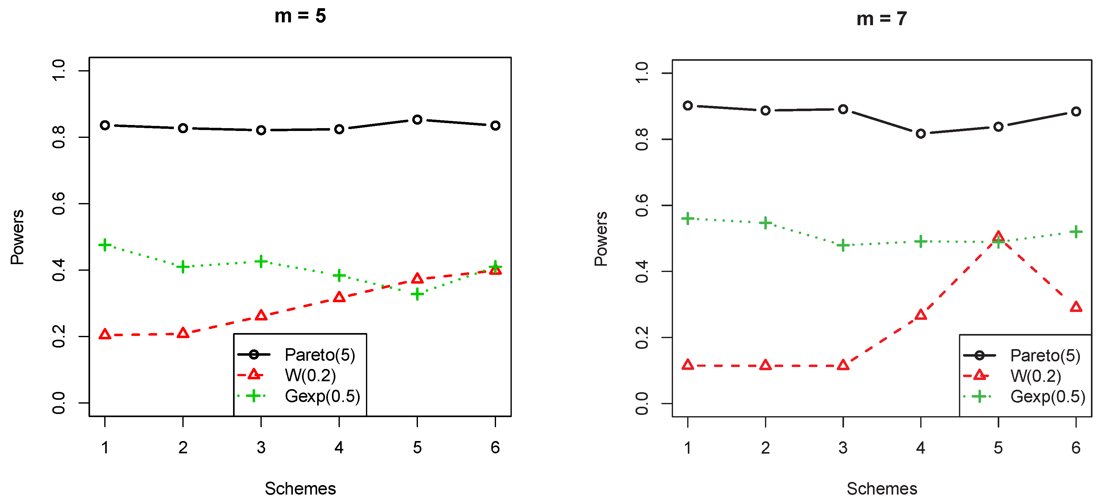
- log-logistic(2) vs. Pareto(5):The shape parameter is , and the failure rate had a downward trend as x increased.
- (b)
- log-logistic(2) vs. Rayleigh(0.2):The shape parameter is , and the failure rate was on the rise as x increased.
- (c)
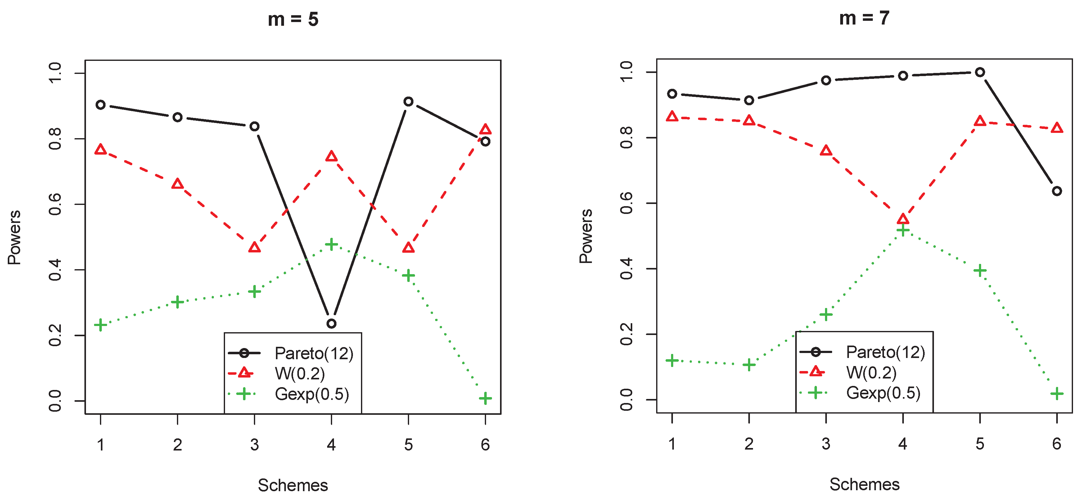
- log-logistic(2) vs. Weibull(0.2,1):where and are the shape parameter and scale parameter corresponding to the distribution, respectively. indicates that the failure rate tended to decrease as the experiment time elapsed. means that the change in failure rate was independent of time. indicates that the failure rate was increasing as the experiment time went on.
- (d)
- log-logistic(2) vs. Bathtub-shaped(2,15):The unknown shape parameter and scale parameter of the distribution are and . In fact, did not have an influence on . This distribution had an increased hazard function when . Otherwise, was bathtub shaped.
- (e)
- log-logistic(2) vs. Gexp(0.5,1):where is the shape parameter and is the scale parameter. The hazard function of this distribution tended to increase when . is constant over time if . When , decreased.
- From Figure 1, different censorship schemes had little effect on power for the test when the hazard function monotonically decreased.
- From Figure 2, for the test, there was no obvious trend in power study for the monotone decreasing hazard function under different censored schemes.
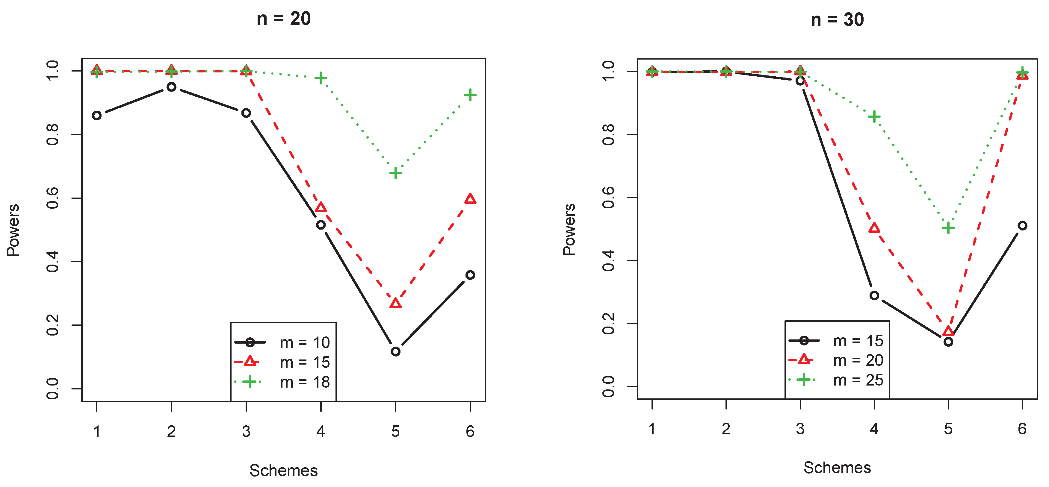
- From Figure 3, when the censorship only happened at the end, the power for the monotone increasing hazard function for the test was lower.
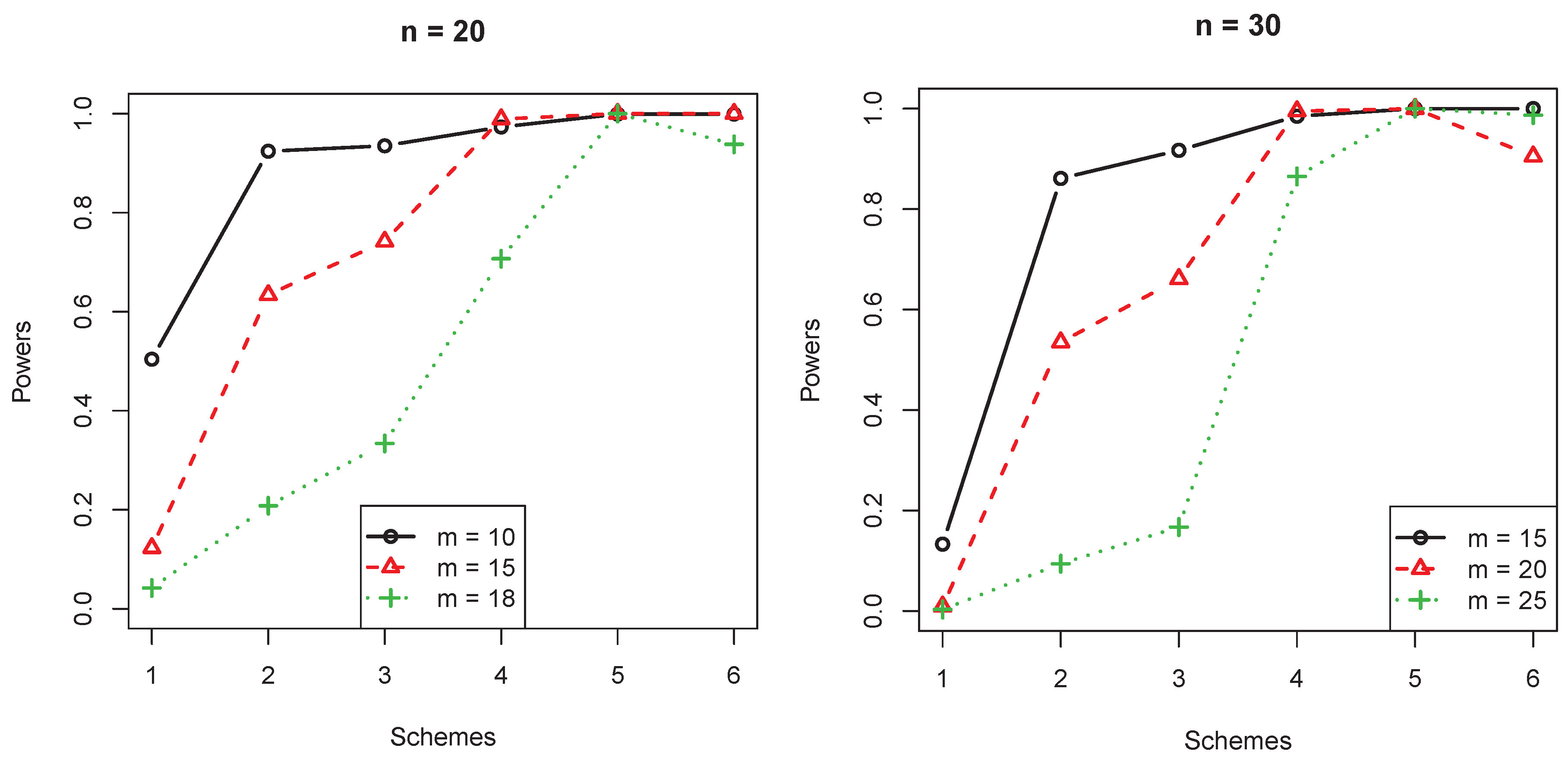
- From Figure 4, when the censorship only happened at the beginning and the hazard function monotonically increased, the power for the test was lower.
6. Illustrative Example
6.1. Application Prospect
6.2. Real Data Application
7. Conclusions
Author Contributions
Funding
Conflicts of Interest
Appendix A
### R code in Monte Carlo simulation
### Randomly generate progressive type-II censored samples
n<-20
m<-10
aa<-1000
r<-c(0,0,0,0,0,0,10,0,0,0)
xx<-matrix(1:(aa*m),aa,m)
for(j in 1:aa){
s<-rexp(m,1)
y<-rep(0,m)
x<-rep(0,m)
y[1]<-s[1]/n
rr<-rep(0,m)
for(i in 1:(m-1)){
rr[1]<-r[1]
rr[i+1]<-rr[i]+r[i+1]
y[i+1]<-y[i]+s[i+1]/(n-rr[i]-i)
i<-i+1
}
### H0:log-logistic(2)
x<-(exp(y)-1)^1/2
xx[j,]<-x
j<-j+1
}
beta1<-rep(0,aa)
for(k in 1:aa){
x1<-xx[k,]
log.like<-function(x,beta){
AA<-m*log(beta)+sum((beta-1)*log(x)-(2+r)*log(1+x^beta))
return(-AA)
}
res<-optim(c(1),log.like,method="L-BFGS-B",lower=0.01,x=x1,
hessian=T,control=list(trace=F,maxit=100))
beta1[k]<-res$par
}
### calculate alpha
alpha<-rep(0,m)
for(i in 1:m){
jj<-seq(m-i+1,m)
alpha[i]<-1-prod((jj+sum(r[jj]))/(jj+sum(r[jj])+1))
i<-i+1
}
#### Find the critical value
A<-rep(0,aa)
B<-rep(0,aa)
C<-rep(0,aa)
D<-rep(0,aa)
E<-rep(0,aa)
crkl<-rep(0,aa)
ckl<-rep(0,aa)
for(j in 1:aa){
xxx<-xx[j,]
beta<-beta1[j]
A[j]<-sum((1-alpha[1:(m-1)])*(xxx[1:(m-1)+1]-xxx[1:(m-1)])
*log(1-alpha[1:(m-1)]))/sum((1-alpha[1:(m-1)])*(xxx[1:(m-1)+1]-xxx[1:(m-1)]))
B[j]<-sum((1-alpha[1:m-1])*(log(xxx[1:(m-1)+1]+xxx[1:(m-1)+1]^(1+beta)
/(1+beta))-log(xxx[1:(m-1)]+xxx[1:(m-1)]^(1+beta)/(1+beta))))
/(sum((1-alpha[1:(m-1)])*(xxx[1:(m-1)+1]-xxx[1:(m-1)])))
C[j]<-(xxx[m]-1/beta*xxx[m]*log(1+xxx[m]^beta)+1/beta*log(xxx[m]
+xxx[m]^(1+beta)/(1+beta)))/(sum((1-alpha[1:(m-1)])*(xxx[1:(m-1)+1]-
xxx[1:(m-1)])))D[j]<-sum(alpha[1:(m-1)]*(xxx[1:(m-1)+1]-xxx[1:(m-1)])
*log(alpha[1:(m-1)]))
/sum((1-alpha[1:(m-1)])*(xxx[1:(m-1)+1]-xxx[1:(m-1)]))
E[j]<-sum(alpha[1:m-1]*(log(xxx[1:(m-1)])-log(xxx[1:(m-1)+1])))
/(sum((1-alpha[1:(m-1)])*(xxx[1:(m-1)+1]-xxx[1:(m-1)])))
j<-j+1
}
crkl<-A+B+C-1
ckl<-D-E-C+1
crkll<-sort(crkl)
ckll<-sort(ckl)
t1<-crkll[aa*0.95]
t2<-ckll[aa*0.95]
t11<-crkll[aa*0.9]
t22<-ckll[aa*0.9]
### calculate power
count1<-rep(0,aa)
count2<-rep(0,aa)
for(j in 1:aa){
z1<-crkl[j]
z2<-ckl[j]
if(z1>=t1) count1[j]<-1
else count1[j]<-0
if(z2>=t2) count2[j]<-1
else count2[j]<-0
j<-j+1
}
power1<-sum(count1)/aa
power2<-sum(count2)/aa
References
- Chen, Z. Estimating the shape parameter of the Log-logistic distribution. Int. J. Reliab. Qual. Saf. Eng. 2006, 13, 257–266. [Google Scholar] [CrossRef]
- Zhou, R.; Sivaganesan, S.; Longla, M. An objective Bayesian estimation of parameters in a log-binomial model. J. Stat. Plan. Inference 2014, 146, 113–121. [Google Scholar] [CrossRef]
- Granzotto, D.C.T.; Louzada, F. The Transmuted Log-Logistic Distribution: Modeling, Inference, and an Application to a Polled Tabapua Race Time up to First Calving Data. Commun. Stat. 2015, 44, 3387–3402. [Google Scholar] [CrossRef]
- Serkan, E. Reliability Properties of Systems with Two Exchangeable Log-Logistic Components. Commun. Stat. 2012, 41, 3416–3427. [Google Scholar]
- Kantam, R.R.L.; Rao, G.S.; Sriram, B. An economic reliability test plan: Log-logistic distribution. J. Appl. Stat. 2006, 33, 291–296. [Google Scholar] [CrossRef]
- Wang, J.; Wu, Z.; Shu, Y.; Zhang, Z. An imperfect software debugging model considering log-logistic distribution fault content function. J. Syst. Softw. 2015, 100, 167–181. [Google Scholar] [CrossRef]
- Surendran, S.; Tota-Maharaj, K. Log logistic distribution to model water demand data. Procedia Eng. 2015, 119, 798–802. [Google Scholar] [CrossRef]
- Cohen, A.C. Progressively censored samples in the life testing. Technometrics 1963, 5, 327–339. [Google Scholar] [CrossRef]
- Román, V.; Balakrishnan, N. Interval Estimation of Parameters of Life From Progressively Censored Data. Technometrics 1994, 36, 84–91. [Google Scholar]
- Balakrishnan, N.; Sandhu, R.A. A Simple Simulational Algorithm for Generating Progressive Type-II Censored Samples. Am. Stat. 1995, 49, 229–230. [Google Scholar]
- Vasicek, O. A test for normality based on sample entropy. J. R. Stat. Soc. 1976, 38, 54–59. [Google Scholar] [CrossRef]
- Taufer, E. On entropy based tests for exponentiality. Commun. Stat. Simul. Comput. 2002, 31, 189–200. [Google Scholar] [CrossRef]
- Noughabi, H.A.; Arghami, N.R. Testing exponentiality based on characterizations of the exponential distribution. J. Stat. Comput. Simul. 2011, 81, 1641–1651. [Google Scholar] [CrossRef]
- Baratpour, S.; Rad, A.H. Exponentiality Test Based on the Progressive Type II Censoring via Cumulative Entropy. Commun. Stat. Simul. Comput. 2016, 45, 2625–2637. [Google Scholar] [CrossRef]
- Kullback, S.; Leibler, R.A. On Information and Sufficiency. Ann. Math. Stat. 1951, 22, 79–86. [Google Scholar] [CrossRef]
- Kullback, S. Information Theory and Statistics; Dover Publicaitons, Inc.: New York, NY, USA, 1959. [Google Scholar]
- Fei, W.; Vemuri, B.C.; Rao, M.; Chen, Y. Cumulative residual entropy, a new measure of information & its application to image alignment. IEEE Trans. Inf. Theory 2004, 50, 1220–1228. [Google Scholar]
- Di Crescenzo, A.; Longobardi, M. On cumulative entropies. J. Stat. Plan. Inference 2009, 139, 4072–4087. [Google Scholar] [CrossRef]
- Park, S.; Rao, M.; Dong, W.S. On cumulative residual Kullback–Leibler information. Stat. Probab. Lett. 2012, 82, 2025–2032. [Google Scholar] [CrossRef]
- Dempster, A.P.; Laird, N.M.; Rubin, D.B. Maximum likelihood from incomplete data via the EM algorithm. J. R. Stat. Soc. 1977, 39, 1–38. [Google Scholar] [CrossRef]
- Sampford, M.R.; Taylor, J. Censored Observations in Randomized Block Experiments. J. R. Stat. Soc. 1959, 21, 214–237. [Google Scholar] [CrossRef]
- Meng, X.L.; Rubin, D.B. Asymptotically optimal estimation for the reduced second moment measure of point processes. Biometrika 1993, 80, 443–449. [Google Scholar]
- Marica, B.; Albéri, M.; Carlo, B. Investigating the potentialities of Monte Carlo simulation for assessing soil water content via proximal gamma-ray spectroscopy. J. Environ. Radioact. 2018, 192, 105–116. [Google Scholar]
- Ma, Y.; Chen, X.; Biegler, L.T. Monte-Carlo-Simulation-based Optimization for Copolymerization Processes with Embedded Chemical Composition Distribution. Comput. Chem. Eng. 2018, 109, 261–275. [Google Scholar] [CrossRef]
- Ni, W.; Li, G.; Zhao, J. Use of Monte Carlo simulation to evaluate the efficacy of tigecycline and minocycline for the treatment of pneumonia due to carbapenemase-producing Klebsiella pneumoniae. Infect. Dis. 2018, 50, 507–513. [Google Scholar] [CrossRef] [PubMed]
- Bormetti, G.; Callegaro, G.; Livieri, G.; Pallavicini, A. A backward Monte Carlo approach to exotic option pricing. Eur. J. Appl. Math. 2018, 29, 146–187. [Google Scholar] [CrossRef]
- Thomas, D.; Wilson, W. Linear Order Statistic Estimation for the Two-Parameter Weibull and Extreme-Value Distributions from Type II Progressively Censored Samples. Technometrics 1972, 14, 679–691. [Google Scholar] [CrossRef]


| Statistics | Hazard Function | Distributions | |
|---|---|---|---|
| 1 | monotone decreasing | Pareto(5); Weibull: W(0.2,1); Generalized exponential distribution: Gexp(0.5,1) | |
| 2 | monotone increasing | Bathtub-shaped: B(2,15) | |
| 3 | monotone decreasing | Pareto(12); Weibull: W(0.2,1); Generalized exponential distribution: Gexp(0.5,1) | |
| 4 | monotone increasing | Rayleigh: R(0.2); Bathtub-shaped: B(2,200) |
| Schemes | ||||||||
|---|---|---|---|---|---|---|---|---|
| n | m | Pareto(5) | W(0.2) | Gexp(0.5) | Pareto(5) | W(0.2) | Gexp(0.5) | |
| 10 | 5 | 5,0,0,0,0 | 0.733 | 0.187 | 0.348 | 0.836 | 0.204 | 0.476 |
| 5 | 0,5,0,0,0 | 0.716 | 0.200 | 0.282 | 0.827 | 0.208 | 0.410 | |
| 5 | 0,0,5,0,0 | 0.674 | 0.238 | 0.322 | 0.821 | 0.261 | 0.426 | |
| 5 | 0,0,0,5,0 | 0.722 | 0.283 | 0.285 | 0.824 | 0.316 | 0.384 | |
| 5 | 0,0,0,0,5 | 0.777 | 0.345 | 0.245 | 0.853 | 0.372 | 0.328 | |
| 5 | 1,1,1,1,1 | 0.711 | 0.378 | 0.336 | 0.835 | 0.399 | 0.410 | |
| 7 | 3,0,0,0,0,0,0 | 0.825 | 0.108 | 0.470 | 0.902 | 0.115 | 0.560 | |
| 7 | 0,3,0,0,0,0,0 | 0.766 | 0.107 | 0.421 | 0.887 | 0.114 | 0.547 | |
| 7 | 0,0,3,0,0,0,0 | 0.722 | 0.104 | 0.361 | 0.891 | 0.114 | 0.479 | |
| 7 | 0,0,0,0,0,3,0 | 0.672 | 0.247 | 0.353 | 0.817 | 0.266 | 0.491 | |
| 7 | 0,0,0,0,0,0,3 | 0.701 | 0.475 | 0.386 | 0.838 | 0.503 | 0.489 | |
| 7 | 1,0,0,1,0,0,1 | 0.770 | 0.265 | 0.379 | 0.884 | 0.290 | 0.520 | |
| 20 | 10 | 10,0,0,0,0,0,0,0,0,0 | 0.918 | 0.068 | 0.585 | 0.969 | 0.074 | 0.704 |
| 10 | 0,10,0,0,0,0,0,0,0,0 | 0.820 | 0.054 | 0.534 | 0.940 | 0.057 | 0.661 | |
| 10 | 0,0,0,0,0,10,0,0,0,0 | 0.866 | 0.106 | 0.419 | 0.937 | 0.114 | 0.580 | |
| 10 | 0,0,0,0,0,0,0,10,0,0 | 0.710 | 0.251 | 0.428 | 0.861 | 0.265 | 0.531 | |
| 10 | 0,0,0,0,0,0,0,0,0,10 | 0.823 | 0.627 | 0.454 | 0.901 | 0.645 | 0.526 | |
| 10 | 1,1,1,1,1,1,1,1,1,1 | 0.793 | 0.349 | 0.515 | 0.911 | 0.372 | 0.638 | |
| 15 | 5,0,0,...,0,0 | 0.980 | 0.026 | 0.714 | 0.992 | 0.029 | 0.880 | |
| 15 | 0,5,0,...,0,0 | 0.959 | 0.018 | 0.681 | 0.987 | 0.023 | 0.813 | |
| 15 | 0,...,0,5,0,...,0 | 0.963 | 0.038 | 0.663 | 0.983 | 0.045 | 0.735 | |
| 15 | 0,0,...,0,5,0 | 0.858 | 0.163 | 0.539 | 0.927 | 0.178 | 0.679 | |
| 15 | 0,0,0,...,0,5 | 0.860 | 0.453 | 0.647 | 0.931 | 0.475 | 0.761 | |
| 15 | 1,1,..,1,...,1,1 | 0.931 | 0.121 | 0.630 | 0.977 | 0.130 | 0.758 | |
| 18 | 2,0,0,...,0,0 | 0.995 | 0.004 | 0.785 | 0.998 | 0.004 | 0.906 | |
| 18 | 0,2,0,...,0,0 | 0.987 | 0.012 | 0.782 | 0.996 | 0.012 | 0.866 | |
| 18 | 0,...,0,2,0,...,0 | 0.987 | 0.017 | 0.738 | 0.994 | 0.018 | 0.861 | |
| 18 | 0,0,...,0,2,0 | 0.985 | 0.035 | 0.704 | 0.996 | 0.038 | 0.806 | |
| 18 | 0,0,0,...,0,2 | 0.967 | 0.082 | 0.694 | 0.994 | 0.092 | 0.803 | |
| 18 | 1,0,0,...,0,1 | 0.993 | 0.039 | 0.752 | 0.999 | 0.040 | 0.873 | |
| 30 | 15 | 15,0,0,...,0,0 | 0.975 | 0.024 | 0.720 | 0.991 | 0.026 | 0.886 |
| 15 | 0,15,0,...,0,0 | 0.930 | 0.020 | 0.651 | 0.978 | 0.024 | 0.795 | |
| 15 | 0,...,0,15,0,...,0 | 0.898 | 0.060 | 0.528 | 0.956 | 0.067 | 0.646 | |
| 15 | 0,0,...,0,15,0 | 0.761 | 0.379 | 0.454 | 0.850 | 0.398 | 0.567 | |
| 15 | 0,0,0,...,0,15 | 0.892 | 0.713 | 0.559 | 0.945 | 0.723 | 0.631 | |
| 15 | 1,1,...,1,...,1 | 0.876 | 0.287 | 0.653 | 0.945 | 0.300 | 0.401 | |
| 20 | 10,0,0,...,0,0 | 0.995 | 0.006 | 0.850 | 0.998 | 0.006 | 0.935 | |
| 20 | 0,10,0,...,0,0 | 0.982 | 0.006 | 0.792 | 0.998 | 0.008 | 0.913 | |
| 20 | 0,...,0,10,0,...0 | 0.978 | 0.013 | 0.734 | 0.992 | 0.016 | 0.848 | |
| 20 | 0,0,...,0,10,0 | 0.843 | 0.282 | 0.566 | 0.913 | 0.297 | 0.694 | |
| 20 | 0,0,0,...,0,10 | 0.898 | 0.712 | 0.666 | 0.947 | 0.740 | 0.779 | |
| 20 | 1,0,1,0,...,0,1,0 | 0.971 | 0.035 | 0.660 | 0.990 | 0.045 | 0.790 | |
| 25 | 5,0,0,...,0,0 | 0.995 | 0.001 | 0.909 | 0.997 | 0.002 | 0.967 | |
| 25 | 0,5,0,...,0,0 | 0.996 | 0.000 | 0.902 | 0.998 | 0.000 | 0.966 | |
| 25 | 0,...,0,5,0,...,0 | 0.989 | 0.002 | 0.827 | 0.998 | 0.003 | 0.935 | |
| 25 | 0,0,...,0,5,0 | 0.955 | 0.054 | 0.718 | 0.986 | 0.066 | 0.813 | |
| 25 | 0,0,0,...,0,5 | 0.977 | 0.163 | 0.780 | 0.999 | 0.182 | 0.910 | |
| 25 | 1,1,..,1,...,1,1 | 0.997 | 0.024 | 0.852 | 0.999 | 0.027 | 0.937 | |
| Schemes | ||||||||
|---|---|---|---|---|---|---|---|---|
| n | m | Pareto(12) | W(0.2) | Gexp(0.5) | Pareto(12) | W(0.2) | Gexp(0.5) | |
| 10 | 5 | 0,5,0,0,0 | 0.786 | 0.602 | 0.161 | 0.904 | 0.765 | 0.232 |
| 5 | 0,0,5,0,0 | 0.678 | 0.424 | 0.195 | 0.866 | 0.660 | 0.302 | |
| 5 | 0,0,0,5,0 | 0.527 | 0.309 | 0.247 | 0.838 | 0.466 | 0.334 | |
| 5 | 0,0,0,0,5 | 0.084 | 0.703 | 0.366 | 0.236 | 0.744 | 0.478 | |
| 5 | 1,1,1,1,1 | 0.449 | 0.369 | 0.272 | 0.914 | 0.465 | 0.383 | |
| 7 | 3,0,0,0,0,0,0 | 0.590 | 0.708 | 0.051 | 0.792 | 0.826 | 0.080 | |
| 7 | 0,3,0,0,0,0,0 | 0.835 | 0.761 | 0.093 | 0.934 | 0.862 | 0.120 | |
| 7 | 0,0,3,0,0,0,0 | 0.828 | 0.712 | 0.077 | 0.914 | 0.850 | 0.107 | |
| 7 | 0,0,0,0,0,3,0 | 0.902 | 0.573 | 0.193 | 0.975 | 0.758 | 0.260 | |
| 7 | 0,0,0,0,0,0,3 | 0.851 | 0.429 | 0.385 | 0.989 | 0.549 | 0.518 | |
| 7 | 1,0,0,1,0,0,1 | 0.983 | 0.684 | 0.276 | 1.000 | 0.848 | 0.395 | |
| 20 | 10 | 10,0,0,0,0,0,0,0,0,0 | 0.376 | 0.711 | 0.007 | 0.637 | 0.827 | 0.019 |
| 10 | 0,10,0,0,0,0,0,0,0,0 | 0.855 | 0.870 | 0.053 | 0.920 | 0.914 | 0.073 | |
| 10 | 0,0,0,0,0,10,0,0,0,0 | 0.814 | 0.728 | 0.065 | 0.929 | 0.828 | 0.099 | |
| 10 | 0,0,0,0,0,0,0,10,0,0 | 0.928 | 0.679 | 0.185 | 0.969 | 0.793 | 0.228 | |
| 10 | 0,0,0,0,0,0,0,0,0,10 | 0.835 | 0.790 | 0.532 | 0.976 | 0.827 | 0.660 | |
| 10 | 1,1,1,1,1,1,1,1,1,1 | 0.998 | 0.707 | 0.370 | 1.000 | 0.859 | 0.506 | |
| 15 | 5,0,0,...,0,0 | 0.045 | 0.659 | 0.002 | 0.193 | 0.803 | 0.002 | |
| 15 | 0,5,0,...,0,0 | 0.494 | 0.883 | 0.004 | 0.717 | 0.927 | 0.005 | |
| 15 | 0,...,0,5,0,...,0 | 0.461 | 0.803 | 0.003 | 0.783 | 0.873 | 0.004 | |
| 15 | 0,0,...,0,5,0 | 0.974 | 0.746 | 0.081 | 0.992 | 0.849 | 0.135 | |
| 15 | 0,0,0,...,0,5 | 1.000 | 0.877 | 0.565 | 0.998 | 0.961 | 0.697 | |
| 15 | 1,1,..,1,...,1,1 | 1.000 | 0.965 | 0.131 | 1.000 | 0.989 | 0.216 | |
| 18 | 2,0,0,...,0,0 | 0.005 | 0.694 | 0.002 | 0.064 | 0.858 | 0.003 | |
| 18 | 0,2,0,...,0,0 | 0.155 | 0.850 | 0.003 | 0.337 | 0.916 | 0.005 | |
| 18 | 0,...,0,2,0,...,0 | 0.122 | 0.793 | 0.002 | 0.384 | 0.880 | 0.002 | |
| 18 | 0,0,...,0,2,0 | 0.547 | 0.793 | 0.001 | 0.848 | 0.896 | 0.004 | |
| 18 | 0,0,0,...,0,2 | 0.999 | 0.974 | 0.095 | 1.000 | 0.993 | 0.158 | |
| 18 | 1,0,0,...,0,1 | 0.913 | 0.937 | 0.005 | 0.980 | 0.966 | 0.011 | |
| 30 | 15 | 15,0,0,...,0,0 | 0.054 | 0.670 | 0.002 | 0.191 | 0.829 | 0.002 |
| 15 | 0,15,0,...,0,0 | 0.798 | 0.903 | 0.012 | 0.876 | 0.956 | 0.015 | |
| 15 | 0,...,0,15,0,...,0 | 0.730 | 0.763 | 0.024 | 0.856 | 0.854 | 0.033 | |
| 15 | 0,0,...,0,15,0 | 0.937 | 0.610 | 0.297 | 0.980 | 0.754 | 0.359 | |
| 15 | 0,0,0,...,0,15 | 0.945 | 0.885 | 0.631 | 1.000 | 0.905 | 0.762 | |
| 15 | 1,1,...,1,...,1 | 1.000 | 0.902 | 0.401 | 1.000 | 0.979 | 0.508 | |
| 20 | 10,0,0,...,0,0 | 0.004 | 0.631 | 0.002 | 0.026 | 0.852 | 0.001 | |
| 20 | 0,10,0,...,0,0 | 0.527 | 0.897 | 0.002 | 0.712 | 0.963 | 0.003 | |
| 20 | 0,...,0,10,0,...0 | 0.448 | 0.815 | 0.003 | 0.666 | 0.914 | 0.004 | |
| 20 | 0,0,...,0,10,0 | 0.993 | 0.712 | 0.174 | 0.999 | 0.885 | 0.269 | |
| 20 | 0,0,0,...,0,10 | 1.000 | 0.632 | 0.669 | 1.000 | 0.802 | 0.779 | |
| 20 | 1,0,1,0,...,0,1,0 | 0.830 | 0.806 | 0.007 | 0.955 | 0.904 | 0.013 | |
| 25 | 5,0,0,...,0,0 | 0.002 | 0.692 | 0.001 | 0.003 | 0.829 | 0.001 | |
| 25 | 0,5,0,...,0,0 | 0.095 | 0.928 | 0.001 | 0.273 | 0.974 | 0.002 | |
| 25 | 0,...,0,5,0,...,0 | 0.054 | 0.853 | 0.000 | 0.221 | 0.931 | 0.001 | |
| 25 | 0,0,...,0,5,0 | 0.894 | 0.781 | 0.003 | 0.988 | 0.911 | 0.011 | |
| 25 | 0,0,0,...,0,5 | 1.000 | 1.000 | 0.600 | 1.000 | 1.000 | 0.722 | |
| 25 | 1,1,..,1,...,1,1 | 0.990 | 0.980 | 0.002 | 1.000 | 0.991 | 0.007 | |
| Schemes | ||||||||
|---|---|---|---|---|---|---|---|---|
| n | m | B(15) | R(0.2) | B(200) | B(15) | R(0.2) | B(200) | |
| 10 | 5 | 5,0,0,0,0 | 0.572 | 0.848 | 0.665 | 0.910 | 0.929 | 0.906 |
| 5 | 0,5,0,0,0 | 0.631 | 0.916 | 0.863 | 0.934 | 0.963 | 0.990 | |
| 5 | 0,0,5,0,0 | 0.557 | 0.841 | 0.300 | 0.841 | 0.954 | 0.793 | |
| 5 | 0,0,0,5,0 | 0.443 | 0.786 | 0.027 | 0.739 | 0.936 | 0.401 | |
| 5 | 0,0,0,0,5 | 0.509 | 0.757 | 0.020 | 0.770 | 0.918 | 0.001 | |
| 5 | 1,1,1,1,1 | 0.420 | 0.854 | 0.041 | 0.688 | 0.968 | 0.405 | |
| 7 | 3,0,0,0,0,0,0 | 0.569 | 0.658 | 0.474 | 0.970 | 0.806 | 0.801 | |
| 7 | 0,3,0,0,0,0,0 | 0.824 | 0.874 | 0.908 | 0.991 | 0.927 | 0.981 | |
| 7 | 0,0,3,0,0,0,0 | 0.859 | 0.911 | 0.924 | 0.992 | 0.964 | 0.987 | |
| 7 | 0,0,0,0,0,3,0 | 0.389 | 0.952 | 0.699 | 0.709 | 0.979 | 0.958 | |
| 7 | 0,0,0,0,0,0,3 | 0.325 | 0.993 | 0.255 | 0.539 | 1.000 | 0.789 | |
| 7 | 1,0,0,1,0,0,1 | 0.404 | 0.992 | 0.966 | 0.729 | 1.000 | 0.998 | |
| 20 | 10 | 10,0,0,0,0,0,0,0,0,0 | 0.860 | 0.358 | 0.127 | 1.000 | 0.504 | 0.488 |
| 10 | 0,10,0,0,0,0,0,0,0,0 | 0.950 | 0.858 | 0.988 | 1.000 | 0.924 | 1.000 | |
| 10 | 0,0,0,0,0,10,0,0,0,0 | 0.868 | 0.884 | 0.962 | 0.997 | 0.935 | 1.000 | |
| 10 | 0,0,0,0,0,0,0,10,0,0 | 0.516 | 0.925 | 0.939 | 0.788 | 0.973 | 0.998 | |
| 10 | 0,0,0,0,0,0,0,0,0,10 | 0.117 | 0.990 | 0.002 | 0.370 | 0.999 | 0.019 | |
| 10 | 1,1,1,1,1,1,1,1,1,1 | 0.358 | 0.995 | 0.999 | 0.645 | 0.999 | 0.999 | |
| 15 | 5,0,0,...,0,0 | 1.000 | 0.042 | 0.008 | 0.999 | 0.123 | 0.067 | |
| 15 | 0,5,0,...,0,0 | 1.000 | 0.463 | 0.536 | 1.000 | 0.634 | 0.846 | |
| 15 | 0,...,0,5,0,...,0 | 0.999 | 0.531 | 0.448 | 1.000 | 0.742 | 0.879 | |
| 15 | 0,0,...,0,5,0 | 0.568 | 0.960 | 0.906 | 0.885 | 0.989 | 0.996 | |
| 15 | 0,0,0,...,0,5 | 0.266 | 1.000 | 0.999 | 0.526 | 1.000 | 1.000 | |
| 15 | 1,1,..,1,...,1,1 | 0.595 | 0.998 | 0.999 | 0.909 | 1.000 | 1.000 | |
| 18 | 2,0,0,...,0,0 | 0.997 | 0.010 | 0.001 | 0.999 | 0.042 | 0.002 | |
| 18 | 0,2,0,...,0,0 | 0.998 | 0.101 | 0.013 | 1.000 | 0.208 | 0.132 | |
| 18 | 0,...,0,2,0,...,0 | 1.000 | 0.137 | 0.014 | 0.996 | 0.334 | 0.160 | |
| 18 | 0,0,...,0,2,0 | 0.978 | 0.422 | 0.141 | 1.000 | 0.707 | 0.596 | |
| 18 | 0,0,0,...,0,2 | 0.679 | 1.000 | 0.996 | 0.955 | 1.000 | 1.000 | |
| 18 | 1,0,0,...,0,1 | 0.925 | 0.803 | 0.548 | 1.000 | 0.938 | 0.872 | |
| 30 | 15 | 15,0,0,...,0,0 | 0.999 | 0.040 | 0.001 | 0.998 | 0.133 | 0.017 |
| 15 | 0,15,0,...,0,0 | 1.000 | 0.750 | 0.922 | 1.000 | 0.861 | 0.990 | |
| 15 | 0,...,0,15,0,...,0 | 0.971 | 0.824 | 0.864 | 0.996 | 0.917 | 0.996 | |
| 15 | 0,0,...,0,15,0 | 0.289 | 0.943 | 0.746 | 0.568 | 0.985 | 0.990 | |
| 15 | 0,0,0,...,0,15 | 0.142 | 1.000 | 0.017 | 0.254 | 1.000 | 0.122 | |
| 15 | 1,1,...,1,...,1 | 0.511 | 1.000 | 1.000 | 0.804 | 1.000 | 1.000 | |
| 20 | 10,0,0,...,0,0 | 0.998 | 0.002 | 0.002 | 0.998 | 0.009 | 0.005 | |
| 20 | 0,10,0,...,0,0 | 0.997 | 0.370 | 0.527 | 0.995 | 0.535 | 0.794 | |
| 20 | 0,...,0,10,0,...0 | 1.000 | 0.487 | 0.566 | 1.000 | 0.661 | 0.898 | |
| 20 | 0,0,...,0,10,0 | 0.501 | 0.977 | 0.987 | 0.734 | 0.995 | 1.000 | |
| 20 | 0,0,0,...,0,10 | 0.173 | 1.000 | 0.997 | 0.368 | 1.000 | 0.999 | |
| 20 | 1,0,1,0,...,0,1,0 | 0.987 | 0.764 | 0.738 | 1.000 | 0.905 | 0.996 | |
| 25 | 5,0,0,...,0,0 | 1.000 | 0.002 | 0.001 | 1.000 | 0.003 | 0.002 | |
| 25 | 0,5,0,...,0,0 | 1.000 | 0.044 | 0.023 | 1.000 | 0.094 | 0.110 | |
| 25 | 0,...,0,5,0,...,0 | 0.999 | 0.088 | 0.014 | 1.000 | 0.167 | 0.108 | |
| 25 | 0,0,...,0,5,0 | 0.857 | 0.658 | 0.309 | 0.999 | 0.865 | 0.886 | |
| 25 | 0,0,0,...,0,5 | 0.504 | 1.000 | 1.000 | 0.836 | 1.000 | 1.000 | |
| 25 | 1,1,..,1,...,1,1 | 0.997 | 0.925 | 0.940 | 1.000 | 0.987 | 0.998 | |
| i | 1 | 2 | 3 | 4 | 5 |
|---|---|---|---|---|---|
| 0.2700 | 1.0224 | 1.5789 | 1.8718 | 1.9947 | |
| 0 | 3 | 0 | 0 | 5 |
© 2019 by the authors. Licensee MDPI, Basel, Switzerland. This article is an open access article distributed under the terms and conditions of the Creative Commons Attribution (CC BY) license (http://creativecommons.org/licenses/by/4.0/).
Share and Cite
Du, Y.; Gui, W. Goodness of Fit Tests for the Log-Logistic Distribution Based on Cumulative Entropy under Progressive Type II Censoring. Mathematics 2019, 7, 361. https://doi.org/10.3390/math7040361
Du Y, Gui W. Goodness of Fit Tests for the Log-Logistic Distribution Based on Cumulative Entropy under Progressive Type II Censoring. Mathematics. 2019; 7(4):361. https://doi.org/10.3390/math7040361
Chicago/Turabian StyleDu, Yuge, and Wenhao Gui. 2019. "Goodness of Fit Tests for the Log-Logistic Distribution Based on Cumulative Entropy under Progressive Type II Censoring" Mathematics 7, no. 4: 361. https://doi.org/10.3390/math7040361
APA StyleDu, Y., & Gui, W. (2019). Goodness of Fit Tests for the Log-Logistic Distribution Based on Cumulative Entropy under Progressive Type II Censoring. Mathematics, 7(4), 361. https://doi.org/10.3390/math7040361