Fractional Order Complexity Model of the Diffusion Signal Decay in MRI

Abstract

Fractional calculus models are steadily being incorporated into descriptions of diffusion in complex, heterogeneous materials. Biological tissues, when viewed using diffusion-weighted, magnetic resonance imaging (MRI), hinder and restrict the diffusion of water at the molecular, sub-cellular, and cellular scales. Thus, tissue features can be encoded in the attenuation of the observed MRI signal through the fractional order of the time- and space-derivatives. Specifically, in solving the Bloch-Torrey equation, fractional order imaging biomarkers are identified that connect the continuous time random walk model of Brownian motion to the structure and composition of cells, cell membranes, proteins, and lipids. In this way, the decay of the induced magnetization is influenced by the micro- and meso-structure of tissues, such as the white and gray matter of the brain or the cortex and medulla of the kidney. Fractional calculus provides new functions (Mittag-Leffler and Kilbas-Saigo) that characterize tissue in a concise way. In this paper, we describe the exponential, stretched exponential, and fractional order models that have been proposed and applied in MRI, examine the connection between the model parameters and the underlying tissue structure, and explore the potential for using diffusion-weighted MRI to extract biomarkers associated with normal growth, aging, and the onset of disease.

1. Introduction

“One of the principal objects of theoretical research in my department of knowledge is to find the point of view from which the subject appears in the greatest simplicity”. J. Willard Gibbs, Letter in Proc. Amer. Acad. Arts & Sci. (1881), pp. 420–421.

Mathematical models are a prism through which we can view the complexity of nature [1]. Just as a prism separates sunlight into the colors of its optical spectrum—portraying hidden features (frequency, intensity, and polarization)—the formulation of a model identifies features not displayed in the raw data. Parameter extraction and estimation mimic a spectrograph by selecting individual spectral components for analysis. In both measurement and modeling, we seek to isolate specific aspects of a physical phenomenon for further study. Success is measured by the degree to which the spectra (or model) captures particular features of the image or visual scene. In paint, the pigments can be identified by a UV-Vis spectrophotometer, but in painting color is described by hue, value, tone, tint, shade, and saturation, all of which are processed by the eye as characteristics of a picture. In modeling biomedical images, we use mathematics to help the brain recognize patterns by identifying new measures of image complexity that convey information in terms of contrast and resolution. Like a spectrograph attached to a telescope or microscope, a mathematical model seeks to capture information hidden in the image of a star or a cell.

Magnetic resonance imaging (MRI) systems are imaging spectrographs that combine camera and spectrometer so as to display the internal structure and composition of the human body [2]. Due to the mismatch between the sub-millimeter resolution of MRI and the sub-micron architecture of biological tissues, mathematical models are needed to describe the mesoscale complexity of living systems. Here, the versatility of MRI offers a variety of tools that encode the mobility of water (molecular rotation and translation) in terms of the magnetic resonance spectrum, and the decay or relaxation of its individual components [3]. In addition, manipulation of the imaging pulse sequence—through modulation of the applied radiofrequency and pulse gradient fields—provides image contrast. Interpretation of this sub-pixel (or for a selected slice, sub-voxel) contrast requires a dynamic model of the local magnetic dipole moment per unit volume, which in the case of diffusion, is the Bloch-Torrey equation [4].

Diffusion-weighted MRI (DW-MRI), based on the Bloch-Torrey equation, is implemented by selective phase encoding within each imaging voxel. This typically involves using a pair of rectangular gradient pulsed (Stejskal-Tanner pulses [5]) to capture the diffusion of water in tissue over the distance of several microns. The DW-MRI signal appears as an exponential signal decay (after appropriate normalization for the local signal intensity and the intrinsic T₁ and T₂ relaxation times) [6]. Hence, the connection between the molecular diffusion coefficient, D (mm²/s) and the detected signal decay involves coarse graining of the magnetic dipole moment per unit volume (M, Amp/m), selection of the transverse component (M_xy), detection of an induced time domain signal (S(t), volts/s), slice selection, phase and spatial encoding to form an image, I(x,y), and finally diffusion encoding into the diffusion signal for each imaging voxel, S(b) = S₀exp(−bD), where diffusion-weighting, b, depends on the pulse gradient strength, g, width, δ, and separation time, Δ, for rectangular Stejskal-Tanner pulses, e.g., b = (γgδ)²(Δ − δ/3), and γ is the gyromagnetic ratio, 42.57 MHz/Tesla for water protons. The analytical solution of the Bloch-Torrey equation is only possible for simple geometries and relatively uniform samples (ideally for Gaussian diffusion in homogenous, isotropic, and unbounded materials) [7]. Relaxation of these conditions leads to the need for additional gradient pulses, which extend the overall imaging time. Hence, the need to simplify this model is guided, on one hand, by a desire to correlate the detected DW-MRI signal with specific tissue features (e.g., isotropic versus anisotropic diffusion or normal versus anomalous diffusion) and on the other by the need to keep the imaging protocol as short as possible—at least in clinical exams.

Anomalous diffusion is characterized by a non-linear growth in the mean squared displacement (MSD) with time [8]. In complex, heterogeneous materials, such as biological tissues, anomalous diffusion has been observed directly in cells and membranes using high resolution optical techniques (fluorescence correlation spectroscopy (FCS), and fluorescence recovery after photobleaching (FRET)), and indirectly in tissues using DW-MRI [9]. Molecular crowding and close cell packing hinder the movement of water reducing the apparent diffusion coefficient from its nominal value of 2.5 × 10⁻³ mm²/s to 0.8 × 10⁻³ mm²/s in brain gray matter, while the MSD remains proportional to the diffusion time [10]. At longer diffusion times (typically greater than 50 ms), the water trapped in and around cells finds its motion not only hindered, but also restricted [11]. For example, water trapped in cells and sub-cellular organelles crosses the associated membranes very slowly and this barrier alters the free diffusion and water transport such that the MSD now increases with time in a sub-linear manner, MSD = 2Dt^α, where 0 < α < 1; a process termed anomalous and sub-diffusive. Both Gaussian (fractional Brownian motion, Langevin equation) and non-Gaussian (continuous time random walk, (CTRW), Lorentz obstructed motion) diffusion models have been suggested describe the DW-MRI data [12]. An example of DW-MRI data is displayed in Figure 1, which is a plot of the normalized signal intensity (S/S₀) versus b-value for white matter (WM), gray matter (GM), and cerebral spinal fluid (CSF) acquired from a normal human brain using a clinical 3 Tesla MRI scanner [13]. The semilogarithmic plot for CSF is the expected straight line characteristic of a single exponential decay. The GM signal exhibits a smaller apparent diffusion coefficient (decay rate) with a small upward curvature at b-values above 1000 s/mm². Hence, both CSF and GM can be described as examples of normal Gaussian diffusion. The WM signal, however, shows a much larger curvature in this plot and a decay rate (slope) that appears to decrease with increasing b-value [14]. Water diffusion in WM is an example of anomalous diffusion where the highly myelinated axons and dense fiber bundles of the white matter add barriers that restrict the movement of tissue water.

Two research paradigms are commonly explored in DW-MRI. First, one can build simplified models of tissue structure by selecting two, three, or four tissue compartments or components, each with a specific, and to be determined, parameter set (e.g., intra- and extra-cellular diffusion and membrane permeability). Diffusion Tensor Imaging (DTI) applies this approach to each image voxel via gradient pulses applied in multiple (at least six) directions. Other approaches (CHARMED, NOODI, AxCaliper, etc.) [15], extend the data collection to multiple b-value shells sampled in hundreds of directions. Alternatively, one can select a heuristic model for S(b), such as the kurtosis, S(b) = S₀exp(−bD)exp[(K/6)(bD)²] [16], or the stretched exponential model, S(b) = S₀ exp[−(bD)^α] [17], and fit the available clinical data to the extended set of model parameters {S₀,D,K} or {S₀,D,α}, respectively. Such models, since they have an extra parameter, will provide an improved fit to S(b) data that extends over multiple b-values. The sword of Damocles in the first approach is the added imaging time, while for the second, it is the dichotomy between the precision of the parameter fit and the ambiguity in the connection between the tissue composition and fitting parameter. Another factor, most often overlooked for both models is the likelihood that the fitting process is degenerate, that is, more than one set of parameters can fit the data with the same least squares fit error [18].

In this paper, we will combine the two modeling approaches described above by using a varying diffusion coefficient D(b) to account for the complexity of the tissue as an inverse power law for higher values of diffusion weighting (b-values), and by generalizing the stretched exponential and kurtosis diffusion decay models by extending the governing diffusion decay to fractional order. The fractional order model naturally accounts for both multiple compartments and non-Gaussian diffusion. After a few preliminary definitions, we will outline an extended form for the fractional diffusion coefficient model, and the corresponding integer and fractional order diffusion decay equations. Examples of the expected functional behavior of the diffusion signal decay as a function of b-value will be plotted and fit to ex vivo bovine optic nerve tissue. In the Discussion we will describe how these models expand the available modeling tools for DW-MRI data and describe how they can be used to fit animal and clinical data. Overall, this approach provides a way to extend the heuristic stretched exponential approach toward more complete multiple-compartment models. This bridge uses fractional order derivatives and varying diffusion coefficients as connecting links.

2. Definitions and Properties

The signals analyzed in DW-MRI, f(b) = S(b)/S₀, are expressed in terms of b, the diffusion-weighting variable defined above for a pair of rectangular diffusion pulses [2,3,4]. Typically, f(b) is a single valued function that is positive, real, and monotonically decreasing for b-values in the range from 0 to 5000 s/mm². For each pixel in an MR image, f(b) is fit to data acquired by varying b in magnitude and gradient direction. The default function used in most DW-MRI is the single exponential, f(b) = exp(−bD). This model reflects the underlying assumptions of a linear, first order relaxation model appropriate for free or hindered Gaussian diffusion. In biological tissues, a sum of exponentials or the stretched exponential, f(b) = exp[(−bD)^α], where 0 < α < 1, is often needed to describe the data, particularly at high b-values. When neither of these approaches are satisfactory, non-Gaussian behavior is considered, and in this paper we will describe it by using a fractional-order relaxation model. Our model involves the Caputo fractional derivative, ^CD^α[f(b)], so below we have defined this derivative operator and its properties. In addition, we also define the Mittag-Leffler function because this function frequently appears in various forms when solving fractional-order differential equations. We will show that the Mittag-Leffler function is also a generalization of the exponential.

2.1. Caputo Fractional Derivative

The simplest description of the non-local, Caputo fractional derivative of order α (0 < α < 1) is as an integral convolution of a power law decay, b^−α/Γ(1 − α), with f(b) [19], hence:

$${}_0{}^{C}D_b^{\alpha }f\left(b\right)=f\left(b\right)\ast \frac{b^{-\alpha }}{\mathsf{\Gamma }\left(1-\alpha \right)} ,$$

(1)

where the gamma function, Γ(z) is defined for all z > 0 by:

$$\mathsf{\Gamma }\left(z\right) = {{\displaystyle \int }}_0^{\infty }{x}^{z-1}{e}^{-x}dx .$$

(2)

For integer values of n, Γ(1 + n) = nΓ(n) = n!, and in the limit as α approaches 1, the Caputo fractional derivative converges to the integer result, ^CD ^α f(b) = df(b)/db. Whereas, for f’(b) = df/db, we have:

$${}_0{}^{C}D_b^{\alpha }f\left(b\right)=\{\begin{array}{c}\frac{1}{\mathsf{\Gamma }\left(1-\alpha \right)}{{\displaystyle \int }}_0^b\frac{1}{{\left(b-b^{\prime }\right)}^{\alpha }} \left(\frac{df\left(b^{\prime }\right)}{d{b}^{\prime }}\right)d{b}^{\prime } 0 < \alpha <1 \\ \frac{df\left(b\right)}{db} \alpha = 1\end{array} ,$$

(3)

Applying the Caputo fractional derivative to monomial of arbitrary degree, к yields:

$${}_0{}^{C}D_b^{\alpha }{b}^{\kappa }= \frac{\mathsf{\Gamma }\left(1+\kappa \right)}{\mathsf{\Gamma }\left(1+\kappa -\alpha \right)}\left( b^{\kappa -\alpha }\right) ,$$

(4)

which gives 1 and 0 for b = 1, and α = 0 and α = 1, respectively. Hence, the Caputo fractional derivative is a simple extension of the integer result db^к/db = [к!/(к − 1)!]b^(к−1)= κ b^(к−1). However, for other common functions, such as the sin(b), cos(b) and exp(b), the results are not quite as simple.

Applying the Caputo fractional derivative term by term to the power series expansion of the single exponential f(b) = exp(b), yields:

$${}_0{}^{C}D_b^{\alpha }\left(e^b\right)= b^{\alpha }\left(e^b\right)\left(1-\frac{\mathsf{\Gamma }\left(-\alpha b\right)}{\mathsf{\Gamma }\left(-\alpha \right)}\right) .$$

(5)

Rather than tabulate all the changes incurred when applying the Caputo fractional derivative to familiar functions, mathematicians have developed particular special functions with simpler behavior under the fractional derivative operation. One such function was defined by the Swedish mathematician, Magnus Gustaf Mittag-Leffer; it is a generalization of the exponential.

2.2. Mittag-Leffer Function

The Mittag-Leffer function, like the Bessel function, comes in different kinds (first, second, modified, etc.), and occurs in both integer and fractional order. It was developed out of the need to simplify the solution of certain classes of ordinary differential equations. Also, like the Bessel function, the Mittag-Leffer function can be defined in terms of a convergent power series. For more information on the Mittag-Leffer function, please consult the monograph by Mainardi and colleagues [20]. There are many versions of the Mittag-Leffler function which subsume almost all of the basic functions of mathematical physics. In this article, we only need three kinds of Mittag-Leffler functions, which we will define in terms of their corresponding power series.

2.3. Exponential Function

Since Γ(n + 1) = n!, the simple decaying exponential has the following power series representation:

$$\exp \left(-b\right)={\displaystyle \sum }_{n=0}^{\infty }\frac{{\left(-b\right)}^n}{\mathsf{\Gamma }\left(n+1\right)} .$$

(6)

2.4. One Parameter Mittag-Leffer Function

The one parameter Mittag-Leffler function [20] is a generalization of the exponential with the parameter, α, inserted a multiplying the integer n. It has the following power series representation:

$${\mathrm{E}}_{\alpha }\left(-b\right)={\displaystyle \sum }_{n=0}^{\infty }\frac{{\left(-b\right)}^n}{\mathsf{\Gamma }\left(n\alpha +1\right)} .$$

(7)

Note, that E₁(−b) = exp(−b) and E₂(−b²) = cos(b).

2.5. Two Parameter Mittag-Leffer Function

The two parameter Mittag-Leffler function [20] includes a second parameter β in the gamma function of the power series as:

$${\mathrm{E}}_{\alpha ,\beta }\left(-b\right)={\displaystyle \sum }_{n=0}^{\infty }\frac{{\left(-b\right)}^n}{\mathsf{\Gamma }\left(n\alpha +\beta \right)} .$$

(8)

Note that here, E_1,1(−b) = exp(−b), E_1,2 (−b) = [1 − exp(−b)]/b, and E_2,2(−b²) = [sin(b)]/b.

2.6. Three Parameter Mittag-Leffer Function

There are several ways to extend the Mittag-Leffler function to three parameters—one credited to Prabhakar [21], and another to Kilbas and Saigo [22]. We will use the Kilbas-Saigo definition, which in power law form can be written as:

$${\mathrm{E}}_{\alpha ,m, l}\left(-b\right)={\displaystyle \sum }_{n=0}^{\infty }{C}_n{\left(-b\right)}^n ,$$

(9)

where c₀ = 1 and:

$$c_n={\displaystyle \prod }_j^{n-1}\frac{\mathsf{\Gamma }\left[\alpha \left(jm+l\right)+1\right]}{\mathsf{\Gamma }\left[\alpha \left(jm+l+1\right)+1\right]} .$$

(10)

Note that E_1,1,1(−b) = exp(−b), E_α,1,1(-b) = E_α(−b), and E_α,β,1(−b) = E_α,β(−b).

Two useful results can be established by applying the Caputo derivative term by term to these power series expressions. First, we find the following for the one parameter Mittag-Leffler function:

$${}_0{}^{C}D_b^{\alpha }{E}_{\alpha }\left[-{\left(bD\right)}^{\alpha }\right]=-D^{\alpha }{E}_{\alpha }\left[-{\left(bD\right)}^{\alpha }\right] .$$

(11)

Thus, the stretched Mittag-Leffler function solves the homogeneous fractional order differential equation ${}_0{}^{C}D_b^{\alpha }y\left(b\right) +D^{\alpha }y\left(b\right)= 0$. And, for α = 1, the above expression reduces to the simple relationship d[exp(−bD)]/db = -D exp(−bD), and gives the solution to the corresponding first order differential equation.

For the inhomogeneous fractional order differential equation:

$${}_0{}^{C}D_b^{\alpha }y\left(b\right)+D^{\alpha }y\left(b\right)= g\left(b\right),$$

(12)

with 0 < α < 1, and y(0) = B, the solution [22] is:

$$y\left(b\right)=B{E}_{\alpha }\left[-{\left(bD\right)}^{\alpha }\right] + {{\displaystyle \int }}_0^b{\left(b-b^{\prime }\right)}^{\alpha -1}{E}_{\alpha ,\alpha }[-{\left(b^{\prime }D\right)}^{\alpha }g\left(b^{\prime }\right)d{b}^{\prime } .$$

(13)

Finally, for the following homogeneous fractional order differential equation:

$${}_0{}^{C}D_b^{\alpha }y\left(b\right)+D^{\alpha }\beta {\left(bD\right)}^{\beta }y\left(b\right)=0 ,$$

(14)

and y(0) = B, the solution [23] is:

$$y\left(b\right)=B{E}_{\alpha ,1+\beta /\alpha ,\beta /\alpha }\left[-{\left(bD\right)}^{\alpha +\beta }\right] ,$$

(15)

which is a reduced form of the three parameter Mittag-Leffler function, with α = α, m = 1 + β/α, and l = β/α. Also, α and β are restricted to the conditions, 0 < α < 1, and − α < β < 1 − α. We will refer to this particular case as the Kilbas-Saigo function in the following text.

3. Results

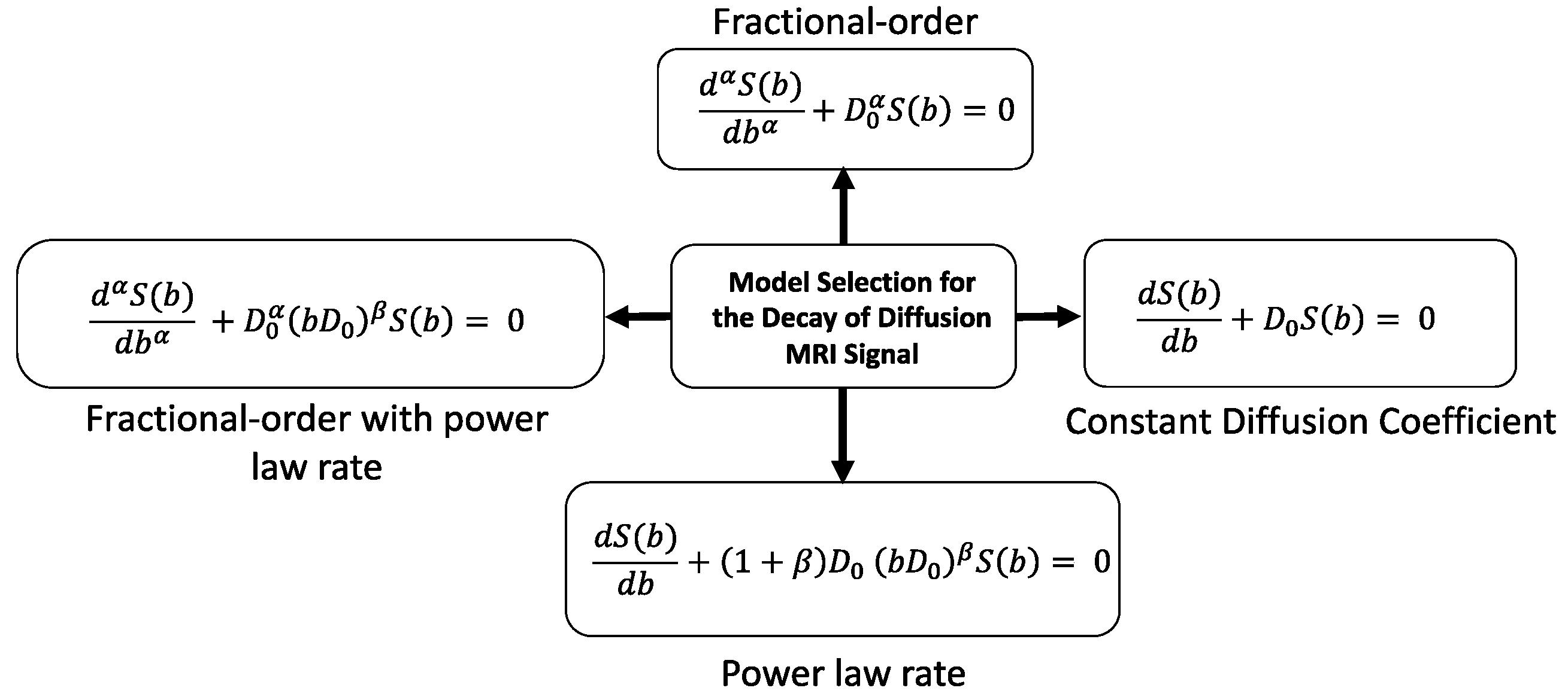
3.1. Fractional Order D(b) Models

A key feature of the anomalous diffusion exhibited in DW-MRI is the fall-off or reduction of the decay rate at b-values above 1000 s/mm². A recent paper [14] surveyed integer order models of this phenomena, where the apparent diffusion coefficient D₀ was expressed as a decaying function of b with a separate decay rate, D₁, for example, D(b) = D₀exp[−(bD₁)]. Here, we focus on fractional order models for systems with both a constant and an inverse power law decay rate. A summary of our approach is given in Figure 2, which illustrates the different integer and fractional order models that will be described. For the integer order case, with a constant diffusion coefficient, D(b) = D₀, the linear differential equation model, yields the classical exponential decay, S(b)/S₀ = exp[−(bD₀)]. A common extension of this model [23,24] assumes an inverse power law decay rate, D(b) = (1 + β)D₀(bD₀)^β, where −1 < β < 0. This integer order, linear differential equation has a stretched exponential solution, S(b)/S₀ = exp[−(bD₀)^(1+β)], which has often been used to fit DW-MRI signals (see, [17,24,25]). The fractional β parameter is zero for the cases of normal and hindered diffusion, as in CSF and gray matter, but less than one for situations where anomalous diffusion appears—such as in brain white matter. Nevertheless, this signal decay model is still exponential, and will decay faster than a power law at high b-values.

Fractional order models asymptotically decay as a power law, so another way to capture the power law tail of the anomalous diffusion signal decay is to consider the decay process to be governed by a Caputo fractional order derivative (order α, with 0 < α < 1) and a constant diffusion coefficient, D₀. The solution for this case is the single parameter stretched Mittag-Leffer function, S(b)/S₀ = E_α[−(bD₀)^α]. This model is attractive because at low b-values it decays as a stretched exponential (approx. 1 − b^α/Γ(1 + α) + …) and at high b-values decays as a power law of the form (b^−α/Γ(1 − α)) [23]. It has been fit to DW-MRI data by Magin, Ingo, and others [12,26]. For completeness, we also show the case of a fractional order Caputo derivative model (order α) with an inverse power law decay rate (order β). The solution for this case is a three parameter Mittag-Leffler function (Kilbas-Saigo form, see Equation (15) and

Table 1. Summary of Diffusion Decay functions, S(b), for Selected Cases.

Constant	Power Law
$S\left(b\right)=S_0\exp \left(-b{D}_0\right)$	$S\left(b\right)=S_0\exp \left(-{\left(b{D}_0\right)}^{1+\beta }\right)$
Mittag-Leffler	Kilbas-Saigo
$S\left(b\right)=S_0{E}_{\alpha }\left(-{\left(b{D}_0\right)}^{\alpha }\right))$	$S\left(b\right)=S_0{E}_{\alpha ,1+\frac{\beta }{\alpha }, \frac{\beta }{\alpha }}\left(-{\left(b{D}_0\right)}^{\alpha +\beta }\right)$

$b={\left(\gamma g\delta \right)}^2\left(\Delta -\frac{\delta }{3}\right), S\left(b=0^{+}\right)=S_0$, where, α, β, and D₀ are constants, and 0 < α < 1, -1 < β < 0.

), but for the inverse power law decay rate is expressed using only α and β as S(b)/S₀ = E_{α,1+β/α,β/α}[-(bD₀)^α+β], [23]. Two things should be noted about this function. First, the conflation of the separate fractional parameters—the α connected with the order of the Caputo fractional derivative, while the β is connected with the presumed inverse power law decay of the diffusion decay rate, D(b). The second thing to note is that, the α and β in this solution are not the α, β of the second order Mittag-Leffler function, but reflect a particular condition on the α, m, and l parameters of the three parameter Mittag-Leffler function. In addition, from its construction, we note that the fractional order derivative with the inverse power law decay rate case includes all of the other models as special cases. All four are displayed in Table 1 for reference and ease of comparison.

In order to display the behavior of the four signal decay models, we have prepared plots of the different diffusion signal decay functions for a selected set of the α and β parameters. The functions were evaluated using MATLAB^® (MathWorks, Natick, MA 01760) and the code is publicly available at [27]. In the MRI field, the stretched exponential was first applied by Bennett et al. [17] to model DW-MRI data. Figure 3 is a plot S(b)/S₀ = exp[−(bD₀)^(1+β)] versus b for b-values between 0 and 4000 s/mm², and D₀ = 1 × 10⁻³ mm²/s. We selected five values for (1 + β) = 0.2, 0.4, 0.6, 0.8, and 1.0. The last value in this sequence, corresponding to β = 0, gives the single exponential function. Three things should be noted about these normalized decay curves. First, they all go through the point f(b) = 0.37 when bD₀ = 1, and for smaller b-values, all the curves fall below the exponential, while for bD₀ > 1, the decay curves are all higher. Thus, the stretched exponential function mimics the combination of a fast plus a slow decay. The deviation from the exponential decreases as the value of (1 + β) increases. Second, slope of the stretched exponential becomes increasingly steep near b = 0, and in fact diverges when (1 + β) < 1. This behavior can be eliminated by shifting the stretched exponential, but that changes the character of the decay [28]. Third, for high b-values, the stretched exponential decays as a power law on a semilogarithmic graph, but not on a linear scale. The multiexponential character of the stretched exponential can be extracted using the inverse Laplace transform (see the work of Berberan-Santos et al., [29]) and it also finds applications in the cumulative function of the Weibull probability distribution [30].

The single parameter Mittag-Leffer function is well known as a relaxation model for dielectric and viscoelastic materials [31,32], and more recently in MRI [12,26]. is a plot S(b)/S₀ = E_α[-(bD₀)^α] versus b for b-values between 0 and 4,000 s/mm², and D₀ = 1 × 10⁻³ mm²/s. We selected five values for α = 0.2, 0.4, 0.6, 0.8, and 1.0. The last value in this sequence, corresponding to α = 1, gives the single exponential function. The one parameter Mittag-Leffler function behaves, overall, in a manner similar to that of the stretched exponential—falling below the exponential at low b-values, and above it at high b-values. However, as shown in Figure 4, all the curves do not pass through bD₀ = 1, but most go through S(b)/S₀ = 0.5 near bD₀ = 0.7. And, for high b-values, on linear scales, the curves flatten out as the α values decrease, reflecting a significant reduction in the apparent diffusion constant—a hallmark of restricted diffusion. On logarithmic scales at high b-values, the one parameter Mittag-Leffler will appear as a straight line, which is characteristic of a pure power decay (see, Carpinteri and Mainardi [31] for these plots). The one parameter Mittag-Leffler has been used to fit DW-MRI data by several groups [12,26] and there is a growing recognition that the fractional order, α, is a homogeneity measure of the sub-voxel tissue environment—as the cellular heterogeneity increases (homogeneity decreases), the α values fall below 1.0. This view is consistent with the spectral distribution model of the one parameter Mittag-Leffler presented by Carpinteri and Mainardi [31], and the inverse Laplace transform analysis of Berberan-Santos [33]. Both models coalesce to a Dirac delta function when α = 1.0, and broaden significantly as α < 1.0, indicating a growing population of compartments with low diffusion rates (coefficients). Hence, one can interpret the one parameter Mittag-Leffler function as a concise multiexponential model of complex, heterogeneous material, and a natural candidate to use when searching for imaging biomarkers of tissue changes or pathology.

The three parameter Mittag-Leffler function (Kilbas-Saigo function), when expressed using only α and β was derived and first applied in MRI by Hanyga and Seredynska [34], but plotted only over a narrow range. Here, we follow the recent work of Capelas de Oliveira, Mainardi, and Vaz [22] and, in addition, suggest that the α and β parameters of the Kilbas-Saigo function might provide separate tissue characterization parameters. We selected different values for α and β subject to the conditions, 0 < α < 1 and 0 < α + β < 1 to ensure complete monotonicity and non-negativity of the spectral distribution [22]. Figure 5 is a plot S(b)/S₀ = E_{α,1+β/α,β/α}[−(bD₀)^α+β] versus b for b-values between 0 and 4000 s/mm², and D₀ = 1 × 10⁻³ mm²/s with α = 1, and β = 0, −0.2, −0.4, −0.6, and −0.8. The signal decay in this case is a weighted stretched exponential and is similar to the stretched exponential case shown in Figure 3 (i.e., S(b)/S₀ = exp[−(1+β)⁻¹(bD₀)^1+β]). Figure 6 is a plot of the Kilbas-Saigo function for the same range of b-values and D₀, but with α = 0.8, and β = 0.2, 0, −0.2, −0.4, and −0.6. In this figure we observe the effects of both α and β on the decay. The fractional derivative order α contributes multiexponential features to the decay, while the power law exponent β influences the low b-values more strongly than the high b-values. Figure 7 is a plot of the Kilbas-Saigo function for the same range of b-values and D₀, but with β = 0.2, and α = 0.2, 0.4, 0.6, 0.8, and 1.0. In the figure, we see for a fixed power law decay of D(b) the shift from lower to higher decay rates as α approaches the exponential function. The separate effects of the two fractional order parameters are also portrayed in the spectral distribution (inverse Laplace transform) of the Kilbas-Saigo function, where for β = 0 (Figure 4 in [22]) decreasing α shifts the spectrum to lower frequencies (smaller D values), which is the basis for the power law tail in the signal decay curve. On the other hand, for fixed α (Figures 5 and 6 in [22]), decreasing β only broadens the distribution about its mean value, which attenuates the diffusion signal in a more uniform manner over the entire range of b-values.

3.2. Fitting Fractional Order D(b) Models to DW-MRI Data

As an example application of these DW-MRI signal decay models, we fit the stretched Kilbas-Saigo function to published ex vivo data acquired from an intact bovine optic nerve [35]. Fits to the exponential, stretched exponential, stretched one parameter Mittag-Leffer were also performed and the results are provided as Supplementary Material. Since the optic nerve consists of bundles of axons, the diffusion signals were measured both along (parallel) and across (perpendicular) the axons. Given the cylindrical structure of the individual nerve axons, we would expect the diffusion to be hindered in the direction along the nerve, and restricted in the direction across the nerve. The Stejskal-Tanner diffusion pulse sequence [5] consists of a pair of rectangular gradient pulses of height g, duration δ, and separation Δ. It was applied by varying the gradient strength, g, and direction for a series of increasing diffusion times (Δ = 8, 10, 20, and 30 ms) with δ set to 3 ms in all cases. The increase in the diffusion time between the gradient pulses can be expected to increase the restricted diffusion contribution for both gradient directions (i.e., when the diffusion length, L_D = (2DΔ)^1/2 exceeds the radius of the axons, typically 5 microns in the parallel case and less than one micron in the perpendicular case). The data was extracted from Figure 1 in [35], and fit using nonlinear least squares optimization in MATLAB^®. The mean squared error was calculated for the Kilbas-Saigo function in both the parallel and perpendicular gradient directions. These results are presented in

Table 2. Summary of Fitting Results for the Stretched Kilbas-Saigo Decay Model.

		Δ = 30 ms	Δ = 20 ms	Δ = 10 ms	Δ = 8 ms
Parallel	D × 104 mm2/s	7.19	7.14	8.86	8.74
Perpendicular		1.95	2.05	2.72	2.75
Parallel	α	0.76	0.75	0.64	0.74
Perpendicular		0.38	0.42	0.38	0.62
Parallel	β	0.06	0.14	0.33	0.26
Perpendicular		0.31	0.27	0.46	0.20
Parallel	Mean-squared error	5.84 × 10−4	5.09 × 10−4	3.47 × 10−4	1.64 × 10−4
Perpendicular		4.38 × 10−4	2.77 × 10−4	2.53 × 10−4	4.61 × 10−4

. As expected, the parallel gradient direction exhibited larger values of the diffusion coefficient than the perpendicular gradient direction (0.72 × 10⁻³ mm²/s versus 0.2 × 10⁻³ mm²/s, when Δ = 30 ms). The stretched Kilbas-Saigo function was able to fit both the parallel and the perpendicular data for all diffusion times. Figure 8 is a plot of the parallel and perpendicular cases when Δ = 30 ms. In the parallel case the α value (ca., 0.75) did not change with increasing diffusion time, while the β value decreased from 0.33 to 0.06. In the perpendicular case, the α value fell from 0.62 to 0.38 with increasing diffusion time, while the β value decreased only from 0.31 to 0.20. These results suggest that the stretched Kilbas-Saigo function is sensitive to both gradient direction and diffusion time. Our goal in this proof of concept paper was only to introduce the Kilbas-Saigo function as a candidate for modeling DW-MRI data. Nevertheless, the nature of the α and β in the model offers the potential of distinguishing between multiexponential (compartmental) contributions via the α parameter and tissue complexity (surface to volume ratio and membrane permeability) contributions through the β parameter. Further analysis of whole imaging slices is needed to establish whether or not this, or another model provides better contrast.

4. Discussion

“One cannot collect all the beautiful shells on the beach” Anne Morrow Lindbergh, Gift from the Sea, 1955.

Fractional calculus interpolates between the integer order operations of calculus just as the real numbers are interspersed between integers. Investigators can employ various fractional derivatives (e.g., Grünwald-Letnikov, Riemann-Liouville, Caputo, Riesz, Hadamard, and Erdélyi-Kober) to stitch together earlier or surrounding data in an extended space-time model of a physical process such as diffusion or dielectric relaxation [19]. The fractional derivatives threads are woven into the model via generalized transcendental functions (Mittag-Leffler, Kilbas-Saigo, Wright, and the H-function of Fox) which are functions that often fit the experimental data with greater fidelity and precision [30,31,32]. In this paper, addressing the decay of diffusion-weighted magnetic resonance signals, we view the problem from a simple perspective—that of a fractional order relaxation with either a fixed or a power-law varying rate constant. The resulting fractional order Kilbas-Saigo model encompasses the simple exponential, the stretched exponential and the stretched Mittag-Leffler function as special cases [21,22,23].

In previous papers, we investigated the challenge of extracting specific complexity measures from DW-MRI data [12,13]. The choices are myriad, while the data is often sparse. Nevertheless, by tuning the applied MR pulse sequence (e.g., by changing the gradient direction or by increasing the diffusion time between gradient pulses) to match a particular aspect of the tissue under study, savings in time and an economy of interpretation are possible. For example, in diffusion tensor imaging (DTI), one uses a simple exponential decay function, but applies the diffusion pulse gradients in six or more directions to capture the anisotropy of skeletal muscle or brain white matter [10]. In a similar manner, in diffusion kurtosis imaging (DKI), by applying gradients in multiple directions and at multiple b-values, the signal decay encodes a measure of restricted diffusion [16]. In some situations, we acquire diffusion trace data to reduce the contributions of tissue anisotropy [36], but extend the range of b-values to 4000 s/mm² or greater to capture aspects of sub-voxel tissue complexity in the fractional order parameters of the Mittag-Leffler function [37,38].

The connection between tissue complexity and the fractional order diffusion decay process is explicit when extremely short diffusion gradient pulses are employed [12,26]. For this situation, the time-space fractional order diffusion equation is known to express—via the Continuous Time Random Walk (CTRW) generalization of Brownian motion—the underlying traps and jumps in the movement of restricted and hindered tissue water. And, while the short gradient pulse duration sequence (Δ > δ) is often applied in laboratory NMR and animal MRI, the larger gradient coils used in human scanners are not currently able to meet this condition. Also, complete mapping of the diffusion signal {g, Δ, δ} carries a time penalty that precludes exploration of a wide range of values in a typical clinical scanning protocol. Hence, an underlying theme in our work is to optimize imaging time, model selection and full data space characterization.

What are the trade-offs between the respective fractional order models (decay functions) considered in the paper? In general, as the b-value increases beyond 1000 s/mm² (e.g., varying g, for fixed Δ and δ) the diffusion regime moves from the domain of hindered diffusion (where diffusion is Gaussian, and the decay is exponential) to one of restricted diffusion (where the diffusion is non-Gaussian, and the decay is often multi-exponential). In the Gaussian case, S(b) = S₀exp[−(bD₀)], we note the reduction in the apparent diffusion coefficient from its value of 2.4 × 10⁻³ mm²/s in cerebral spinal fluid to 0.8 × 10⁻³ mm²/s in brain gray matter by a tortuosity factor of 3, so the apparent diffusion coefficient, ADC = D_CSF/3. For intermediate b-values (1000–3000 s/mm²), the stretched exponential decay function, S(b) = S₀ exp[−(bD₀)^α], can be used, but so can a bi-exponential model, a kurtosis model or the varying diffusion coefficient (VDC) model where D(b) = D₀ exp(−bD₁) [14,39]. When the b-values increase above 3000 s/mm², the exponential models all rapidly decay while the signal often persists due to trapped tissue water, which exhibits an inverse power law decrease in signal intensity. This behavior can be captured by the VDC model, but it is also naturally encoded in the Mittag-Leffler decay, S(b) = S₀E_α[−(bD₀)^α], which for low b-values approximates the stretched exponential, and for high b-values decays asymptotically as (bD₀)^−α. The Kilbas-Saigo generalization of the Mittag-Leffer function is the mother function (model) for all three cases, and has been applied before by Hanyga and Seredynska [34] to diffusion in MRI and by Lin to problems in NMR [40,41]. The behavior of the Kilbas-Saigo modeling approach for the case of varying Δ (for fixed g and δ) has not yet been fully examined. Here, we were successful in capturing the anisotropy of the bovine optic nerve and the emergence of anomalous diffusion as the diffusion time increases. These results are similar to the behavior of the q-space model, S(b) = S₀E_α[−D_α,β q^β(Δ−δ/3)^α], where q = (γgδ)/2π is a measure of the strength of the diffusion gradient phase encoding [26]. Future such studies would involve normal and tumor tissues and could employ oscillating diffusion gradients for short times and stimulated echo imaging for long times.

The motivation for fractional calculus models of diffusion signal decay in MRI has both a practical and a theoretical basis [42]. The practical emerges from advances in diffusion−weighted imaging sequences that use stronger gradients (b-values, above 2000 s/mm²) to probe sub-voxel tissue compartments. The signal from regions with relatively unhindered diffusion (e.g., cerebral spinal fluid) decays very quickly, while the signal from regions exhibiting pronounced hindered and restricted diffusion persists. Researchers and clinicians fit these signals to a variety of models (e.g., multi-exponential, stretched exponential, and kurtosis) to account for the change in the apparent diffusion coefficient as the b-value increases—fits that provide additional imaging biomarkers of sub-voxel structure [43,44,45]. In this ongoing effort, the medical community seeks to link the model parameters to changes in tissue due to local and diffuse disease. The theoretical basis for considering fractional calculus models emerges from the growing recognition in the biophysics community of the prevalence of anomalous diffusion—due to molecular crowding—in cells and cell membranes [8,9]. Mathematical models of anomalous diffusion include Gaussian models (Brownian and fractional Brownian motion), Langevin equations, the non-Gaussian CTRW, and Lorentz obstructed transport models [46,47]. Within this group, there is a recurrence of power law behavior in the statistics of stochastic models, the correlation coefficients of dynamic models and the waiting time and jump increment probabilities in non-Gaussian models. Since the integral and differential operators of fractional calculus naturally accommodate power laws, via convolution, it is not surprising that anomalous diffusion can be cast in the mathematical language of fractional calculus. Alternatively, the diffusion process can be described by generalizing the diffusion constant into a diffusion coefficient that is a function of either b-value or diffusion time.

5. Conclusions

In this paper, we described DW-MRI signal decay using sub-diffusion models that can be expressed simply in terms of b-value: exponential, stretched exponential, Mittag-Leffler and Kilbas-Saigo. The stretched Kilbas-Saigo function encompasses this set, and depending on the gradient direction and range of b-values acquired in the experiment, can fit the data with three parameters: (i) D₀, the apparent diffusion coefficient; (ii) α, the order of the fractional derivative; and (iii) β, the fractional exponent of the inverse power law decay of D(b). The goal was to illustrate how this model can capture the anomalous decay of S(b) observed when data collected over a range of diffusion times. The resulting model parameters encode aspects of the sub-voxel tissue structure, hence offer the potential for describing changes that are brought about by the onset of disease or the success of treatment.

References

1. Gershenfeld, N. The Nature of Mathematical Modeling; Cambridge University Press: Cambridge, UK, 1999; 344p. [Google Scholar]
2. Haacke, E.M.; Brown, R.W.; Thompson, M.R.; Venkatesan, R. Magnetic Resonance Imaging: Physical Principles and Sequence Design; Wiley-Blackwell: New York, NY, USA, 1999; 914p. [Google Scholar]
3. Jones, D.K. Diffusion MRI: Theory, Methods, and Applications; Oxford University Press: Oxford, UK, 2011; 748p. [Google Scholar]
4. Callaghan, P.T. Translational Dynamics and Magnetic Resonance: Principles of Pulsed Gradient Spin Echo NMR; Oxford University Press: Oxford, UK, 2011; 568p. [Google Scholar]
5. Stejskal, E.O.; Tanner, J.E. Spin diffusion measurements: Spin echoes in the presence of a time-dependent field gradient. J. Chem. Phys. 1965, 42, 288–292. [Google Scholar] [CrossRef]
6. Liang, Z.-P.; Lauterbur, P.C. Principles of Magnetic Resonance Imaging: A Signal Processing Approach; Wiley—IEEE Press: Piscataway, NJ, USA, 1999; 416p. [Google Scholar]
7. Kimmich, R. NMR: Tomography, Diffusometry, Relaxometry; Springer: New York, NY, USA, 1997; 526p. [Google Scholar]
8. Bouchaud, J.-P.; Georges, A. Anomalous diffusion in disordered media: Statistical mechanisms, models and physical applications. Phys. Rep. 1990, 195, 127–293. [Google Scholar] [CrossRef]
9. Höfling, F.; Franosch, T. Anomalous transport in the crowded world of biological cells. Rep. Prog. Phys. 2013, 76, 046602. [Google Scholar] [CrossRef] [PubMed] [Green Version]
10. Mori, S.; Tournier, J.D. Introduction to Diffusion Tensor Imaging: And Higher Order Models; Academic Press: New York, NY, USA, 2013; 126p. [Google Scholar]
11. Price, W.S. NMR Studies of Translational Motion: Principles and Applications; Cambridge University Press: Cambridge, UK, 2009; 393p. [Google Scholar]
12. Magin, R.L.; Ingo, C.; Colon-Perez, L.; Triplett, W.; Mareci, T.H. Characterization of anomalous diffusion in porous biological tissues using fractional order derivatives and entropy. Microporous Mesoporous Mater. 2013, 178, 39–43. [Google Scholar] [CrossRef]
13. Magin, R.L.; Abdullah, O.; Baleanu, D.; Zhou, X.J. Anomalous diffusion expressed through fractional order differential operators in the Bloch-Torrey equation. J. Magn. Reson. 2008, 190, 255–270. [Google Scholar] [CrossRef] [PubMed]
14. Magin, R.L. Models of diffusion signal decay in magnetic resonance imaging: Capturing complexity. Concepts Magn. Reson. 2016, 45A, 21401. [Google Scholar] [CrossRef]
15. Alexander, D.C.; Hubbard, P.L.; Hall, M.G.; Moore, E.A.; Ptito, M.; Parker, G.J.M.; Dyrby, T.B. Orientationally invariant indices of axon diameter and density from diffusion MRI. Neuroimage 2010, 52, 1374–1389. [Google Scholar] [CrossRef] [PubMed]
16. Jensen, J.H.; Helpern, J.A.; Ramani, A.; Lu, H.; Kaczynski, K. Diffusional kurtosis imaging: The quantification of non-Gaussian water diffusion by means of magnetic resonance imaging. Magn. Reson. Med. 2005, 53, 1432–1440. [Google Scholar] [CrossRef]
17. Bennett, K.M.; Schmaidna, K.M.; Bennett, R.; Rowe, D.B.; Lu, H.; Hyde, J.S. Characterization of continuously distributed cortical water diffusion rates with a stretched-exponential model. Magn. Reson. Med. 2003, 50, 727–734. [Google Scholar] [CrossRef] [Green Version]
18. Jelescu, I.O.; Veraart, J.; Fieremans, E.; Novikov, D.S. Degeneracy in model parameter estimation for multi-compartmental diffusion in neuronal tissue. NMR Biomed. 2016, 29, 33–47. [Google Scholar] [CrossRef] [PubMed]
19. Podlubny, I. Fractional Differential Equations; Academic Press: New York, NY, USA, 1999; 368p. [Google Scholar]
20. Gorenflo, R.; Kilbas, A.A.; Mainardi, F.; Rogosin, S.V. Mittag-Leffler Functions, Related Topics and Applications; Springer-Verlag: Berlin, Germany, 2014; 443p. [Google Scholar]
21. Kilbas, A.A.; Saigo, M.; Saxena, R.K. Generalized Mittag-Leffler function and generalized fractional calculus operators. Integr. Trans. Spec. Funct. 2004, 15, 31–49. [Google Scholar] [CrossRef]
22. de Oliveira, E.C.; Mainardi, F.; Vaz, J. Fractional models of anomalous relaxation based on the Kilbas and Saigo function. Meccanica 2014, 49, 2049–2060. [Google Scholar] [CrossRef]
23. Kilbas, A.A.; Srivastava, H.M.; Trujillo, J.J. Theory and Applications of Fractional Differential Equations; Elsevier: Amsterdam, The Netherlands, 2006; 523p. [Google Scholar]
24. Hall, M.G.; Barrick, T.R. From diffusion-weighted MRI to anomalous diffusion imaging. Magn. Reson. Med. 2008, 59, 447–455. [Google Scholar] [CrossRef] [Green Version]
25. Berberan-Santos, M.N. A luminescence decay function encompassing the stretched exponential and the compressed hyperbola. Chem. Phys. Lett. 2008, 460, 146–150. [Google Scholar] [CrossRef] [Green Version]
26. Ingo, C.; Magin, R.L.; Colon-Perez, L.; Triplett, W.; Mareci, T.H. On random walks and entropy in diffusion weighted magnetic resonance imaging studies of neural tissue. Magn. Reson. Med. 2014, 71, 617–627. [Google Scholar] [CrossRef]
27. R.L.M. Kilbas and Saigo Function. Available online: https://www.mathworks.com/matlabcentral/fileexchange/70999-kilbas-and-saigo-function (accessed on 12 March 2018).
28. Berberan-Santos, M.N.; Bodunov, E.N.; Valeur, B. Mathematical functions for the analysis of luminescence decays with underlying distributions: 1. Kohlrausch decay function (stretched exponential). Chem. Phys. 2005, 315, 171–182. [Google Scholar] [CrossRef]
29. Berberan-Santos, M.N.; Valeur, B. Luminescence decays with underlying distributions: General properties and analysis with mathematical functions. J. Lumin. 2007, 126, 263–272. [Google Scholar] [CrossRef]
30. Spanier, J.; Oldham, K.B. An Atlas of Functions; Hemisphere Publishing Corp: New York, NY, USA, 1987; pp. 253–262. [Google Scholar]
31. Carpinteri, A.; Mainardi, F. Fractals and Fractional Calculus in Continuum Mechanics CISM Courses and Lectures No. 378; Springer-Wien: New York, NY, USA, 1997; 348p. [Google Scholar]
32. Hilfer, R. (Ed.) Applications of Fractional Calculus in Physics; World Scientific: Singapore, 2007; 472p. [Google Scholar]
33. Berberan-Santos, M.N. Relation between the inverse Laplace transforms of I(tb) and I(t): Application to the Mittag-Leffler and asymptotic inverse power law relaxation functions. J. Math. Chem. 2005, 38, 265–270. [Google Scholar] [CrossRef]
34. Hanyga, A.; Seredynska, M. Anisotropy in high-resolution diffusion-weighted MRI and anomalous diffusion. J. Magn. Reson. 2012, 220, 85–93. [Google Scholar] [CrossRef]
35. Stanisz, G.J.; Szafer, A.; Wright, G.A.; Henkelman, R.M. An analytical model of restricted diffusion in bovine optic nerve. Magn. Reson. Med. 1997, 37, 103–111. [Google Scholar] [CrossRef]
36. Zhou, X.J.; Gao, Q.; Abdullah, O.; Magin, R.L. Studies of anomalous diffusion in the human brain using fractional order calculus. Magn. Reson. Med. 2010, 63, 562–569. [Google Scholar] [CrossRef] [Green Version]
37. Sui, Y.; He, W.; Damen, F.W.; Wanamaker, C.; Li, Y.; Zhou, X.J. Differentiation of low- and high-grade pediatric brain tumors with high b-value diffusion weighted MR imaging and a fractional order calculus model. Radiology 2015, 277, 489–496. [Google Scholar] [CrossRef]
38. Karaman, M.M.; Sui, Y.; Wang, H.; Magin, R.L.; Li, Y.; Zhou, X.J. Differentiating low- and high-grade pediatric brain tumors using a continuous-time random-walk diffusion model at high b-values. Magn. Reson. Med. 2016, 76, 1149–1157. [Google Scholar] [CrossRef]
39. Magin, R.L.; Karaman, M.M.; Hall, M.G.; Zhu, W.; Zhou, X.J. Capturing complexity of the diffusion-weighted MR signal decay. Magn. Reson. Imaging 2019, 56, 110–118. [Google Scholar] [CrossRef]
40. Lin, G. Analysis of PFG anomalous diffusion via real-space and phase-space approaches. Mathematics 2018, 6, 17. [Google Scholar] [CrossRef]
41. Lin, G. Describe NMR relaxation by anomalous rotational or translational diffusion. Commun. Nonlinear Sci. Numer. Simul. 2019, 72, 232–239. [Google Scholar] [CrossRef]
42. Novikov, D.S.; Kiselev, V.G.; Jespersen, S.N. On modeling. Magn. Reson. Med. 2018, 79, 317–3193. [Google Scholar] [CrossRef]
43. Grebenkov, D.S. From the microstructure to diffusion NMR, and back. In Diffusion NMR of Confined Systems: Fluid Transport in Porous Solids and Heterogeneous Materials; Valiullin, R., Ed.; The Royal Society of Chemistry: Cambridge, UK, 2017; pp. 52–110. [Google Scholar]
44. Grinberg, F.; Farrher, F.; Shah, N.J. Diffusion magnetic resonance imaging in brain tissue. In Diffusion NMR of Confined Systems: Fluid Transport in Porous Solids and Heterogeneous Materials; Valiullin, R., Ed.; The Royal Society of Chemistry: Cambridge, UK, 2017; pp. 497–528. [Google Scholar]
45. Topgaard, D. Multidimensional diffusion MRI. J. Magn. Reson. 2019, 275, 98–113. [Google Scholar] [CrossRef]
46. Klages, R.; Radons, G.; Sokolov, I.M. (Eds.) Anomalous Transport: Foundations and Applications; Wiley-VCH: Weinheim, Germany, 2008; 583p. [Google Scholar]
47. Evangelista, L.R.; Lenzi, E.K. Fractional Diffusion Equations and Anomalous Diffusion; Cambridge Univ. Press: Cambridge, UK, 2018; 345p. [Google Scholar]
Figure 1. Normalized signal intensity plotted versus b for selected regions of interest (ROI) in white matter (WM), gray matter (GM) and cerebrospinal fluid (CSF) for a human brain (reprinted from ref. [13] with permission). DW-EPI T2-weighted image at 3.0 Tesla, TR/TE = 4000/97 ms, FOV = 22 cm · 22 cm, matrix 128 ·72 (zero padded to 256 · 256 during image reconstruction), in plane resolution = 1.72 mm × 3.05 mm and slice thickness = 4 mm. The experimental data were fit to the fractional order stretched exponential model, S(b) = S0exp[(−bD)α)], (WM, α = 0.64, D = 0.41 × 10⁻³ mm2/s ; GM, α = 0.82, D = 0.66 × 10⁻³ mm2/s ; CSF, α = 0.95, D = 2.72 × 10⁻³ mm2/s).
Mathematics 07 00348 g001
Figure 2. A diagram illustrating four approaches selected for generalization of the classical Gaussian model of diffusion-weighted signal attenuation in magnetic resonance imaging (MRI) (integer or fractional order, each with a constant diffusion coefficient or one with an inverse power law decay). An example of a representative differential equation for S(b) is shown for each case.
Mathematics 07 00348 g002
Figure 3. The normalized signal decay of S(b)/S0 for a stretched exponential decay is plotted for b-values between 0 and 4000 s/mm2, and D0 = 1 × 10⁻³ mm2/s. Five values for (1 + β) = 0.2, 0.4, 0.6, 0.8, and 1.0 are displayed. The last value in this sequence gives the single exponential function. As the value of (1 + β) moves toward 1, the shape of the decay curve transitions from a multiple exponential with fast and slow components to a single exponential decay.
Mathematics 07 00348 g003
Figure 4. The normalized stretched Mittag-Leffler signal decay of S(b)/S0 is plotted versus b-values between 0 and 4000 s/mm2, with D0 = 1 × 10⁻³ mm2/s. Five values for α = 0.2, 0.4, 0.6, 0.8, and 1.0 are displayed. The last value in this sequence, corresponding to α = 1, gives the single exponential function. As the value of α decreases, the shape of the decay curve transitions from stretched exponential to an asymptotic power law decay.
Mathematics 07 00348 g004
Figure 5. The normalized stretched Kilbas-Saigo signal decay of S(b)/S0 is plotted versus b-values between 0 and 4000 s/mm2, and D0 = 1 × 10⁻³ mm2/s with α = 1, and β = 0, −0.2, −0.4, −0.6, and −0.8. The signal decay in the α = 1 case is a weighted stretched exponential. As the value of β decreases, the shape of the decay curve transitions from a stretched exponential decay to a pattern with a asymptotic power law decay.
Mathematics 07 00348 g005
Figure 6. The normalized stretched Kilbas-Saigo signal decay of S(b)/S0 is plotted versus b-values between 0 and 4000 s/mm2, and D0 = 1 × 10⁻³ mm2/s with α = 0.8, and β = 0.2, 0, −0.2, −0.4, and −0.6. In this figure, we observe the effects of both α and β on the decay.
Mathematics 07 00348 g006
Figure 7. The normalized stretched Kilbas-Saigo signal decay of S(b)/S0 is plotted versus b-values between 0 and 4000 s/mm2, and D0 = 1 × 10⁻³ mm2/s with β = 0.2, and α = 0.2, 0.4, 0.6, 0.8, and 1.0. In the figure, we see for a fixed power law decay of D(b) the shift from lower to higher decay rates as α approaches the exponential function.
Mathematics 07 00348 g007
Figure 8. An example of the normalized stretched Kilbas-Saigo signal decay fits of S(b)/S0 to the bovine optic nerve data for the parallel and perpendicular directions with Δ = 30 ms. The photomicrographs are from [35] and are used with permission from the journal Magnetic Resonance in Medicine.
Mathematics 07 00348 g008