Interval-Valued Probabilistic Hesitant Fuzzy Set Based Muirhead Mean for Multi-Attribute Group Decision-Making

Abstract

As a powerful generalization to fuzzy set, hesitant fuzzy set (HFS) was introduced, which provided multiple possible membership values to be associated with a specific instance. But HFS did not consider occurrence probability values, and to circumvent the issue, probabilistic HFS (PHFS) was introduced, which associates an occurrence probability value with each hesitant fuzzy element (HFE). Providing such a precise probability value is an open challenge and as a generalization to PHFS, interval-valued PHFS (IVPHFS) was proposed. IVPHFS provided flexibility to decision makers (DMs) by associating a range of values as an occurrence probability for each HFE. To enrich the usefulness of IVPHFS in multi-attribute group decision-making (MAGDM), in this paper, we extend the Muirhead mean (MM) operator to IVPHFS for aggregating preferences. The MM operator is a generalized operator that can effectively capture the interrelationship between multiple attributes. Some properties of the proposed operator are also discussed. Then, a new programming model is proposed for calculating the weights of attributes using DMs’ partial information. Later, a systematic procedure is presented for MAGDM with the proposed operator and the practical use of the operator is demonstrated by using a renewable energy source selection problem. Finally, the strengths and weaknesses of the proposal are discussed in comparison with other methods.

1. Introduction

Multi-attribute group decision-making (MAGDM) is an interesting and complex day-to-day problem which involves implicit uncertainty and vagueness [1]. Hesitant fuzzy set (HFS) [2] is a powerful extension of the fuzzy set [3] that allows multiple degrees of truth to be associated with each preference information for better handling uncertainty and vagueness. Attracted by the strength of HFS, many researchers used HFS for different MAGDM applications viz., supplier selection [4,5], plant location selection [6], hospital site selection [7] and pattern recognition [8]. Recently, Rodriguez et al. [9] conducted a thorough analysis of HFS and some of its variants and identified its usefulness in MAGDM.

Though HFS is powerful, it lacks the ability to consider occurrence probability for each hesitant fuzzy element (HFE). To alleviate the issue, Xu and Zhou [10] put forward the probabilistic hesitant fuzzy set (PHFS), which associates occurrence probability value for each HFE. Motivated by the power of PHFS, researchers widely explored the idea for multi-attribute decision-making (MADM) [11,12,13,14,15,16,17]. Though PHFS alleviates the weakness of HFS to some extent, still the elicitation of occurrence probability is prone to imprecision and inaccuracy. To circumvent the weakness, a generalized model called interval-valued PHFS (IVPHFS) [18] is put forward which associates a range of values as occurrence probability to each HFE with a constraint that the sum of upper limit probability equals unity. As a generalization of Reference [18], Krishankumar et al. [19] proposed an IVPHFS concept which associates a range of values as occurrence probability for each HFE (for flexible elicitation of occurrence probability values). This mitigates the problem of imprecision and inaccuracy in the elicitation of occurrence probability values by providing multiple choices of values as occurrence probability for each HFE.

Based on the literature analysis of PHFS, we can infer that IVPHFS is a recent extension to PHFS which needs to be better explored for effective MAGDM. Group decision-making (GDM) [20] is a widely studied problem which obtains preference information from multiple DMs and aggregates them into single preference information without much loss of information. Mesiar et al. [21] made an interesting analysis of aggregation functions and we can infer that the realization of the interrelationship between attributes is a key factor for aggregation operators. Most of the state-of-the-art operators ignore this theme and are hence, not very suitable for MAGDM.

The MM [22] operator is an aggregation operator that reflects the interrelationship between attributes in a better way by considering risk appetite (refer Section 3 for details)s. MM is a generalized operator which can easily represent other operators viz., arithmetic average, geometric average, generalized arithmetic average, Bonferroni mean [23] and Maclaurin symmetric mean [24] as special cases.

Some challenges that can be encountered from the literature analysis made above are:

• Elicitation of occurrence probability in a precise manner is difficult and prone to inaccuracies.
• Following this, aggregation of preference information with better scope to capture the interrelationship between attributes is an open challenge in the IVPHFS context.
• Further, calculation of weights of attributes by making reasonable use of partial information from DMs is also an open challenge.
• Understanding the applicability, strengths and weaknesses of the proposed method are also substantial for effective use of the framework in uncertain situations.

Motivated by these challenges and to circumvent the same, in this paper, some key contributions are made:

• As a generalization to PHFS, IVPHFS [18,19] was proposed which allows the range of occurrence probability values to be associated with each HFE. This mitigates the issue of imprecision and inaccuracy in probability elicitation and addresses challenge (1).
• MM operator is extended in the IVPHFS context for capturing the interrelationship between attributes in a better way. Also, DMs’ preferences are aggregated in a rational manner by considering risk appetite along with the weight of each DM which addresses challenge (2).
• A new mathematical programming model is put forward in the IVPHFS context for calculation of weights of attributes with the help of partial information from the DMs. The idea is to use this partial information effectively for a reasonable calculation of weights.
• The applicability of the proposed method is validated by using a green supplier selection problem.
• Finally, the superiority and weakness of the proposed method are discussed in comparison with other methods.

The rest of the paper is constructed as follows. Section 2 describes some basic concepts of HFS, PHFS and IVPHFS. Section 3 presents the core idea of the research in which the proposed aggregation operator along with some desirable properties is discussed. Further, a new programming model is put forward for calculating attributes’ weight values and finally, a systematic procedure is presented for MAGDM using proposed aggregation operator. In Section 4, a numerical example for green supplier selection is put forward to validate the applicability of the proposed method. In Section 5, some superiority and weakness of the proposal are discussed by comparison with other methods and finally, in Section 6, concluding remarks with future research directions are presented.

2. Preliminaries

Let us discuss some basics of HFS, PHFS and IVPHFS concepts.

Definition 1

[2]. Consider a fixed set $T$ and hesitant fuzzy set (HFS) $H$ on $T$ which is a function $h$ that produces a subset in the interval $\left[0,1\right]$. Mathematically, it is given by,

$$H=\left(t,h_H\left(t\right)|t\in T\right)$$

(1)

where $h_H\left(t\right)$ is the set of values in range 0 to 1.

Remark 1.

For convenience, $h_H\left(t\right)=h\left(t\right)$ is called the hesitant fuzzy element (HFE) and the collection of HFEs is $H$.

Definition 2

[10]. Consider a fixed set $T$. The PHFS $H_p$ on $T$ is given by,

$$H_P=\left(t,h_{H_p}\left({\gamma }_i,p_i\right)|t\in T\right)$$

(2)

where $h_{H_p}\left({\gamma }_i,p_i\right)$ is the probabilistic hesitant fuzzy element with ${\gamma }_i$ being the membership value of $t$ with its associated occurrence probability $p_i$ and $i=1,2,\dots ,\#h_{H_p}$.

Remark 2.

For convenience, $h_{H_p}\left({\gamma }_i,p_i\right)=h\left({\gamma }_i,p_i\right)$ is called the probabilistic hesitant fuzzy element (PHFE) with ${\gamma }_i$ and $p_i$ in the range 0 to 1.

Definition 3

[19]. Consider a fixed set $T$. The IVPHFS $H_{IP}$ on $T$ is given by,

$$H_{IP}=\left(t,h_{H_p}\left({\gamma }_i,\left[p_i^l,p_i^u\right]\right)\right)$$

(3)

where $h_{H_p}\left({\gamma }_i,\left[p_i^l,p_i^u\right]\right)$ is the interval-valued probabilistic hesitant fuzzy element with ${\gamma }_i$ being the membership value of $t$ with its associated occurrence probability value in the interval fashion as $\left[p_i^l,p_i^u\right]$, for all $i=1,2,\dots ,\#h_{H_{Ip}}$.

Here, ${\gamma }_i$, $p_i^l$ and $p_i^u$ are in the range 0 to 1 and $p_i^l\le p_i^u$. For simplicity, $h_{H_p}\left({\gamma }_i,\left[p_i^l,p_i^u\right]\right)=h\left({\gamma }_i,\left[p_i^l,p_i^u\right]\right)=h$ is called interval-valued probabilistic hesitant fuzzy element (IVPHFE).

Consider an example where a DM provides his preference for ice-creams. Initially, he uses PHFS information (refer Definition 2) to rate different ice-creams viz., vanilla, strawberry and chocolate as $H_P=\left(vennila,\left\{0.6,\left(0.4\right)\right\},strawberry,\left\{0.8,\left(0.5\right)\right\},chocolate,\left\{0.4,\left(0.7\right)\right\}\right)$. Later, he uses IVPHFS information (refer Definition 3) to provide probability values in a more flexible manner. $H_{IP}=\left(vennila,\left\{0.6,\left[0.3,0.45\right]\right\},strawberry,\left\{0.8,\left[0.4,0.6\right]\right\},,chocolate,\left\{0.4,\left[0.6,0.7\right]\right\}\right)$. By applying the latter style for preference information, we can increase the flexibility by providing a range of values as probability values.

Definition 4

[19]. Let $h_1$, $h_2$ and $h_3$ be three IVPHFEs; then some operations are given by,

$$h_1⨁h_2=\left({\gamma }_1+{\gamma }_2-{\gamma }_1{\gamma }_2,\left[p_1^l{p}_2^l,p_1^u{p}_2^u\right]\right)$$

(4)

$$h_1⨂h_2=\left({\gamma }_1{\gamma }_2,\left[p_1^l{p}_2^l,p_1^u{p}_2^u\right]\right)$$

(5)

$$\lambda h_1=\left(1-{\left(1-{\gamma }_1\right)}^{\lambda },\left[p_1^l,p_1^u\right]\right)$$

(6)

$$h_1^{\lambda }=\left({\gamma }_1^{\lambda },\left[p_1^l,p_1^u\right]\right)$$

(7)

Here, Equations (4)–(7) represent addition, multiplication, scalar multiplication and power operations. Actually, these equations are algebraic Archimedean T-norm and T-conorm and the additive generators used here are $g\left(x\right)=-ln\left(x\right)$ for T-norm $T_A\left(x,y\right)=xy$ and $h\left(x\right)=-ln\left(1-x\right)$ for T-conorm $S_A\left(x,y\right)=x+y-xy$.

• Property 1: Commutativity

  $$h_1⨁h_2=h_2⨁h_1$$

  $$h_1⨂h_2=h_2⨂h_1$$
• Property 2: Associativity

  $$h_1⨁\left(h_2⨁h_3\right)=\left(h_1⨁h_2\right)⨁h_3$$

  $$h_1⨂\left(h_2⨂h_3\right)=\left(h_1⨂h_2\right)⨂h_3$$

3. Proposed Methodology

3.1. IVPHFS Based MM Operator and Its Properties

This section presents a new extension to the popular and powerful MM operator in the IVPHFS context. The MM operator [22] is a generalized operator which aggregates preferences by properly capturing the interrelationship between attributes. The operator can be used to realize other operators as mentioned above. The MM operator also considers the risk appetite values of DMs along with their relative importance (weights) in its formulation which intuitively produces a rational aggregation of preference information.

Table 1. Review of MM operator on different fuzzy sets.

Ref.#	Aggregation Operator	Preference Style	Attributes’ Weights Calculation	Applications
[25]	MM	Picture fuzzy set	no	Investment risk
[26]	Power MM	T-spherical fuzzy set	no	Air quality evaluation
[27]	MM	The hesitant fuzzy linguistic term set	no	ERP system selection
[28]	MM	Hesitant fuzzy set	no	Evaluation of emergency responses
[29]	Power MM	Neutrosophic cubic fuzzy set	no	Van selection
[30]	MM	Pythagorean fuzzy set	no	Airline evaluation
[31]	MM	q-rung orthopair fuzzy set	no	Investor selection
[32]	MM	The probabilistic linguistic term set	no	Project selection

provides a review on MM operators that are proposed for different fuzzy sets. This provides an idea on the basic concept of MM operator, its practical use in MADM problems. Moreover, the challenges mentioned above are clearly supported by this tabular analysis.

From Table 1, it can be inferred that (i) preference styles either associate a single value as a probability or ignore probability, which is not reasonable for decision-making; (ii) the MM operator is popularly used for aggregating preference information by effectively capturing the interrelationship between attributes and (iii) finally, attributes’ weight values are directly (not calculated) obtained from the DMs which causes inaccuracies in the decision-making process.

Motivated by the power of MM operator and IVPHFS concept, in this paper, we extend the MM operator to IVPHFS and the definition and properties are given below:

Definition 5.

The aggregation of IVPHFEs using IVPHFMM (interval-valued probabilistic hesitant fuzzy Muirhead mean) operator is a mapping from $T^k\to T$ for $k=1,2,\dots ,nd$ which is given by,

$$\begin{array}{c}IVPHFM{M}^{\left({\lambda }_1,{\lambda }_2,\dots ,{\lambda }_{nd}\right)}\left(h_1,h_2,\dots ,h_{nd}\right)\\ \hfill =\left(\begin{array}{c}{\left({\displaystyle \prod }_{k=1}^{nd}{\left({\displaystyle \prod }_{j=1}^{nd}{\gamma }_i^{{\lambda }_j}\right)}^{w_k}\right)}^{\frac{1}{{{\displaystyle \sum }}_j{\lambda }_j}},\\ [{\left({\displaystyle \prod }_{k=1}^{nd}{\left({\displaystyle \prod }_{j=1}^{nd}{\left(p_i^l\right)}^{{\lambda }_j}\right)}^{w_k}\right)}^{\frac{1}{{{\displaystyle \sum }}_j{\lambda }_j}},{\left({\displaystyle \prod }_{k=1}^{nd}{\left({\displaystyle \prod }_{j=1}^{nd}{\left(p_i^u\right)}^{{\lambda }_j}\right)}^{w_k}\right)}^{\frac{1}{{{\displaystyle \sum }}_j{\lambda }_j}}]\end{array}\right)\end{array}$$

(8)

where ${\lambda }_1,{\lambda }_2,\dots ,{\lambda }_k$ is risk appetite values of each DM from the set $\left\{1,2,\dots ,nd\right\}$, $nd$ is the total number of DMs, $w_k$ is the weight of the $k^{th}$ DM.

It must be noted that Equation (8) provides the MM operator in the IVPHFS context. The operator aggregates the membership values, followed by the probability values (in the interval fashion). That is, the lower limit of the probability value is aggregated and then the upper limit of the probability value is aggregated. The square bracket represents the interval values that we obtain upon aggregation of probability values. Further, we present a theorem below to show that aggregation of different IVPHFEs by using IVPHFMM operator produces an IVPHFE.

Remark 3.

The MM operator is initially proposed in Reference [22] and it is given by ${\left(\frac{1}{nd!}{\displaystyle \sum }_{k=1}^{nd}{\displaystyle \prod }_{j=1}^{nd}{a}_k^{{\lambda }_j}\right)}^{\frac{1}{{{\displaystyle \sum }}_j{\lambda }_j}}$ where $nd$ is the number of DMs and ${\lambda }_j$ is the risk appetite values for $j=1,2,\dots ,nd$. Risk appetite is defined by ISO 31000 as the amount of risk pursued, retained or taken by an organization. In this case, it is the risk pursued, retained or taken by a DM. The possible values are from the set $\left\{1,2,\dots ,nd\right\}$. The higher the value of $\lambda$ indicates a higher risk appetite value for the DM.

Property 1: Idempotent

If IVPHFEs $h_1=h_2=\dots =h_k=h$, then $IVPHFM{M}^{\left({\lambda }_1,{\lambda }_2,\dots ,{\lambda }_k\right)}\left(h_1,h_2,\dots ,h_k\right)=h$.

Proof. 

From Equation (8),

$$\begin{gathered} IVPHFM{M}^{\left({\lambda }_1,{\lambda }_2,\dots ,{\lambda }_k\right)}\left(h_1,h_2,\dots ,h_k\right)=\left(\begin{array}{c}{\left({\displaystyle \prod }_{k=1}^{nd}{\left({\displaystyle \prod }_{j=1}^{nd}{\gamma }_i^{{\lambda }_j}\right)}^{w_k}\right)}^{\frac{1}{{{\displaystyle \sum }}_j{\lambda }_j}},\\ [{\left({\displaystyle \prod }_{k=1}^{nd}{\left({\displaystyle \prod }_{j=1}^{nd}{\left(p_i^l\right)}^{{\lambda }_j}\right)}^{w_k}\right)}^{\frac{1}{{{\displaystyle \sum }}_j{\lambda }_j}},{\left({\displaystyle \prod }_{k=1}^{nd}{\left({\displaystyle \prod }_{j=1}^{nd}{\left(p_i^u\right)}^{{\lambda }_j}\right)}^{w_k}\right)}^{\frac{1}{{{\displaystyle \sum }}_j{\lambda }_j}}]\end{array}\right) \\ =\left(\begin{array}{c}{\left({\displaystyle \prod }_{k=1}^{nd}{\left({\gamma }_i^{{\lambda }_1+{\lambda }_2+\dots +{\lambda }_{nd}}\right)}^{w_k}\right)}^{\frac{1}{{{\displaystyle \sum }}_j{\lambda }_j}},\\ [{\left({\displaystyle \prod }_{k=1}^{nd}{\left({\left(p_i^l\right)}^{{\lambda }_1+{\lambda }_2+\dots +{\lambda }_{nd}}\right)}^{w_k}\right)}^{\frac{1}{{{\displaystyle \sum }}_j{\lambda }_j}},{\left({\displaystyle \prod }_{k=1}^{nd}{\left({\left(p_i^u\right)}^{{\lambda }_1+{\lambda }_2+\dots +{\lambda }_{nd}}\right)}^{w_k}\right)}^{\frac{1}{{{\displaystyle \sum }}_j{\lambda }_j}}]\end{array}\right) \end{gathered}$$

By doing the same to DMs’ weight values, we obtain, $\begin{array}{l}=\left(\begin{array}{c}{\left({\gamma }_i^{{\lambda }_1+{\lambda }_2+\dots +{\lambda }_{nd}}\right)}^{\frac{1}{{{\displaystyle \sum }}_j{\lambda }_j}},\\ \left[{\left({\left(p_i^l\right)}^{{\lambda }_1+{\lambda }_2+\dots +{\lambda }_{nd}}\right)}^{\frac{1}{{{\displaystyle \sum }}_j{\lambda }_j}},{\left({\left(p_i^u\right)}^{{\lambda }_1+{\lambda }_2+\dots +{\lambda }_{nd}}\right)}^{\frac{1}{{{\displaystyle \sum }}_j{\lambda }_j}}\right]\end{array}\right)\\ =\left({\gamma }_i,\left[p_i^l,p_i^u\right]\right)=h\end{array}$ as ${\displaystyle \sum }_k{w}_k=1$. □

Property 2: Commutativity

If $h_i^{*}$ is any permutation of $h_i \forall i=1,2,\dots ,k$, then $IVPHFM{M}^{\left({\lambda }_1,{\lambda }_2,\dots ,{\lambda }_k\right)}\left(h_1,h_2,\dots ,h_k\right)=IVPHFM{M}^{\left({\lambda }_1,{\lambda }_2,\dots ,{\lambda }_k\right)}\left(h_1^{*},h_2^{*},\dots ,h_k^{*}\right)$.

Proof. 

$$\begin{gathered} IVPHFM{M}^{\left({\lambda }_1,{\lambda }_2,\dots ,{\lambda }_k\right)}\left(h_1^{*},h_2^{*},\dots ,h_k^{*}\right)=\left(\begin{array}{c}{\left({\displaystyle \prod }_{k=1}^{nd}{\left({\displaystyle \prod }_{j=1}^{nd}{\gamma }_i^{*{\lambda }_j}\right)}^{w_k}\right)}^{\frac{1}{{{\displaystyle \sum }}_j{\lambda }_j}},\\ [{\left({\displaystyle \prod }_{k=1}^{nd}{\left({\displaystyle \prod }_{j=1}^{nd}{\left(p_i^{*l}\right)}^{{\lambda }_j}\right)}^{w_k}\right)}^{\frac{1}{{{\displaystyle \sum }}_j{\lambda }_j}},{\left({\displaystyle \prod }_{k=1}^{nd}{\left({\displaystyle \prod }_{j=1}^{nd}{\left(p_i^{*u}\right)}^{{\lambda }_j}\right)}^{w_k}\right)}^{\frac{1}{{{\displaystyle \sum }}_j{\lambda }_j}}]\end{array}\right) \\ =\left(\begin{array}{c}{\left({\displaystyle \prod }_{k=1}^{nd}{\left({\displaystyle \prod }_{j=1}^{nd}{\gamma }_i^{{\lambda }_j}\right)}^{w_k}\right)}^{\frac{1}{{{\displaystyle \sum }}_j{\lambda }_j}},\\ [{\left({\displaystyle \prod }_{k=1}^{nd}{\left({\displaystyle \prod }_{j=1}^{nd}{\left(p_i^l\right)}^{{\lambda }_j}\right)}^{w_k}\right)}^{\frac{1}{{{\displaystyle \sum }}_j{\lambda }_j}},{\left({\displaystyle \prod }_{k=1}^{nd}{\left({\displaystyle \prod }_{j=1}^{nd}{\left(p_i^u\right)}^{{\lambda }_j}\right)}^{w_k}\right)}^{\frac{1}{{{\displaystyle \sum }}_j{\lambda }_j}}]\end{array}\right)=IVPHFM{M}^{\left({\lambda }_1,{\lambda }_2,\dots ,{\lambda }_k\right)}\left(h_1,h_2,\dots ,h_k\right) \end{gathered}$$

 □

Property 3: Monotonicity

Consider IVPHFEs $h^{\prime }=h_i^{\prime }$ and $h=h_i$ for $i=1,2,\dots ,k$ such that $h_i^{\prime }\ge h_i$. Then, $IVPHFM{M}^{\left({\lambda }_1,{\lambda }_2,\dots ,{\lambda }_k\right)}\left(h_1,h_2,\dots ,h_k\right)\le IVPHFM{M}^{\left({\lambda }_1,{\lambda }_2,\dots ,{\lambda }_k\right)}\left(h_1^{\prime },h_2^{\prime },\dots ,h_k^{\prime }\right)$.

Proof. 

Let ${\gamma }_i^{\prime }={\left({\displaystyle \prod }_{k=1}^{nd}{\left({\displaystyle \prod }_{j=1}^{nd}{\left({\gamma }_i^{\prime }\right)}^{{\lambda }_j}\right)}^{w_k}\right)}^{\frac{1}{{{\displaystyle \sum }}_j{\lambda }_j}}$ and $\left[p_i^{l\prime },p_i^{u\prime }\right]=\left[{\left({\displaystyle \prod }_{k=1}^{nd}{\left({\displaystyle \prod }_{j=1}^{nd}{\left(p_i^{l\prime }\right)}^{{\lambda }_j}\right)}^{w_k}\right)}^{\frac{1}{{{\displaystyle \sum }}_j{\lambda }_j}},{\left({\displaystyle \prod }_{k=1}^{nd}{\left({\displaystyle \prod }_{j=1}^{nd}{\left(p_i^{u\prime }\right)}^{{\lambda }_j}\right)}^{w_k}\right)}^{\frac{1}{{{\displaystyle \sum }}_j{\lambda }_j}}\right]$. Similarly, $h_i$ is defined as above. Now score and deviation measure is adopted from Reference [19] for IVPHFEs. Since $h_i^{\prime }\ge h_i$ $\forall i=1,2,\dots ,k$, $s\left(h^{\prime }\right)\ge s\left(h\right)$ which concludes that $h^{\prime }\ge h$ and if $s\left(h^{\prime }\right)=s\left(h\right)$, then calculate deviation and if $\sigma \left(h\right)\ge \sigma \left(h^{\prime }\right)$ $h^{\prime }\ge h$. Thus, $IVPHFM{M}^{\left({\lambda }_1,{\lambda }_2,\dots ,{\lambda }_k\right)}\left(h_1,h_2,\dots ,h_k\right)\le IVPHFM{M}^{\left({\lambda }_1,{\lambda }_2,\dots ,{\lambda }_k\right)}\left(h_1^{\prime },h_2^{\prime },\dots ,h_k^{\prime }\right)$. □

Property 4: Bounded

For any IVPHFE $h_i \forall i=1,2,\dots ,k$, $h^{-}\le IVPHFM{M}^{\left({\lambda }_1,{\lambda }_2,\dots ,{\lambda }_k\right)}\left(h_1,h_2,\dots ,h_k\right)\le h^{+}$. Here, $h^{-}=min\left(h_i\right)$ and $h^{+}=max\left(h_i\right)$. Initially, $\frac{{\gamma }_i{p}_i^l+{\gamma }_i{p}_i^u}{2}$ is calculated and the IVPHFE that correspond to minimum and maximum value is considered as h⁻ and $h^{+}$ respectively.

Proof. 

Based on the monotonic and idempotent property of IVPHFMM operator, we can easily conclude that $IVPHFM{M}^{\left({\lambda }_1,{\lambda }_2,\dots ,{\lambda }_k\right)}\left(h_1,h_2,\dots ,h_k\right)\ge IVPHFM{M}^{\left({\lambda }_1,{\lambda }_2,\dots ,{\lambda }_k\right)}\left(h^{-},h^{-},\dots ,h^{-}\right)$. Similarly, $IVPHFM{M}^{\left({\lambda }_1,{\lambda }_2,\dots ,{\lambda }_k\right)}\left(h_1,h_2,\dots ,h_k\right)\le IVPHFM{M}^{\left({\lambda }_1,{\lambda }_2,\dots ,{\lambda }_k\right)}\left(h^{+},h^{+},\dots ,h^{+}\right)$. Combining these two inequalities, we get $h^{-}\le IVPHFM{M}^{\left({\lambda }_1,{\lambda }_2,\dots ,{\lambda }_k\right)}\left(h_1,h_2,\dots ,h_k\right)\le h^{+}$. □

Theorem 1.

The aggregation of IVPHFEs by IVPHFMM operator produces an IVPHFE.

Proof. 

To prove the above theorem, we must show that the aggregated value obeys Definition 3. Now, from Property 4, it is clear that the aggregated value is bounded within the different IVPHFEs taken for aggregation. By extending the idea further, we get $0\le {\left({\displaystyle \prod }_{k=1}^{\#DM}{\left({\displaystyle \prod }_{j=1}^{\#DM}{\gamma }_i^{{\lambda }_j}\right)}^{w_k}\right)}^{\frac{1}{{{\displaystyle \sum }}_j{\lambda }_j}}\le 1$ and $0\le \begin{array}{c}\left[{\left({\displaystyle \prod }_{k=1}^{\#DM}{\left({\displaystyle \prod }_{j=1}^{\#DM}{\left(p_i^l\right)}^{{\lambda }_j}\right)}^{w_k}\right)}^{\frac{1}{{{\displaystyle \sum }}_j{\lambda }_j}},{\left({\displaystyle \prod }_{k=1}^{\#DM}{\left({\displaystyle \prod }_{j=1}^{\#DM}{\left(p_i^u\right)}^{{\lambda }_j}\right)}^{w_k}\right)}^{\frac{1}{{{\displaystyle \sum }}_j{\lambda }_j}}\right]\end{array}\le 1$. By combining these two inequalities, we get $0\le (\begin{array}{c}{\left({\displaystyle \prod }_{k=1}^{\#DM}{\left({\displaystyle \prod }_{j=1}^{\#DM}{\gamma }_i^{{\lambda }_j}\right)}^{w_k}\right)}^{\frac{1}{{{\displaystyle \sum }}_j{\lambda }_j}},\\ \begin{array}{c}\left[{\left({\displaystyle \prod }_{k=1}^{\#DM}{\left({\displaystyle \prod }_{j=1}^{\#DM}{\left(p_i^l\right)}^{{\lambda }_j}\right)}^{w_k}\right)}^{\frac{1}{{{\displaystyle \sum }}_j{\lambda }_j}},{\left({\displaystyle \prod }_{k=1}^{\#DM}{\left({\displaystyle \prod }_{j=1}^{\#DM}{\left(p_i^u\right)}^{{\lambda }_j}\right)}^{w_k}\right)}^{\frac{1}{{{\displaystyle \sum }}_j{\lambda }_j}}\right]\end{array}\end{array}\le 1$. Thus, $0\le IVPHFM{M}^{\left({\lambda }_1,{\lambda }_2,\dots ,{\lambda }_k\right)}\left(h_1,h_2,\dots ,h_k\right)\le 1$. Hence, aggregation of IVPHFEs yields an IVPHFE. □

3.2. Weight Calculation for Attributes Using the Proposed Programming Model

This section put forwards a new mathematical programming model in the IVPHFS context for calculating the weights of attributes. There are mainly two types of weight calculation methods. In the first type, weight values are calculated with completely unknown information and some popular examples are analytical hierarchy process (AHP) [33], entropy measure [34] and so forth. In the second type, weight values are calculated with partially known information and this type of weight calculation gives DMs a chance to express their personal preference on each attribute which is considered during the weight calculation process. Whenever partial information is known for each attribute, the effective idea is to use the information for rational calculation of weights.

Motivated by the ability of the second type of weight calculation, in this paper, a new programming model is put forward in the IVPHFS context. The key advantages of the proposed model are (i) it uses the partial information from the DMs in a rational manner in its formulation; (ii) provides flexibility to the DMs to share their personal preferences on each attribute in the form of constraints; (iii) the nature of the attribute (benefit or cost) is also taken into consideration during formulation and (iv) the ideal solution for each attribute is considered for rational calculation of weight values which resemble closely to the human cognition process.

The systematic procedure for attribute weight calculation is presented below:

Step 1:

Construct an evaluation matrix of order $3\times 4$ with IVPHFS information. The order of the matrix is DMs by attributes.

Step 2:

Calculate the positive ideal solution (PIS) and negative ideal solution (NIS) for each attribute using Equations 9 and 10.

$$h_j^{PIS}=ma{x}_{j\in benefit}\left({{\displaystyle \sum }}_{i=1}^{\#h}{\gamma }_i\left(\frac{p_i^l+p_i^u}{2}\right)\right)\left(\mathrm{or}\right)mi{n}_{j\in cost}\left({{\displaystyle \sum }}_{i=1}^{\#h}{\gamma }_i\left(\frac{p_i^l+p_i^u}{2}\right)\right)$$

(9)

$$h_j^{NIS}=mi{n}_{j\in benefit}\left({{\displaystyle \sum }}_{i=1}^{\#h}{\gamma }_i\left(\frac{p_i^l+p_i^u}{2}\right)\right)\left(\mathrm{or}\right)ma{x}_{j\in cost}\left({{\displaystyle \sum }}_{i=1}^{\#h}{\gamma }_i\left(\frac{p_i^l+p_i^u}{2}\right)\right)$$

(10)

where $h_j^{PIS}$ and $h_j^{NIS}$ are PIS and NIS values of the $j^{th}$ attribute respectively.

The $h_j^{PIS}$ and $h_j^{NIS}$ are calculated for each attribute and they contain IVPHFS information of the corresponding value obtained from Equations 9 and 10.

Step 3:

Apply Model 1 to obtain the weights of attributes.

Model 1:

$$Min Z={\displaystyle \sum }_{j=1}^n{w}_j{\displaystyle \sum }_{i=1}^{m}d\left(h_{ij},h_j^{PIS}\right)-d\left(h_{ij},h_j^{NIS}\right)$$

Subject to:

$$0\le w_j\le 1;{{\displaystyle \sum }}_j{w}_j=1.$$

The distance measure is calculated using Equation (11).

$$d\left(a,b\right)=\sqrt{{\displaystyle \sum }_{i=1}^{\#instance}{\left(\left({\gamma }_{ia}\left(\frac{p_{ia}^l+p_{ia}^u}{2}\right)\right)-\left({\gamma }_{ib}\left(\frac{p_{ib}^l+p_{ib}^u}{2}\right)\right)\right)}^2}$$

(11)

where $a$ and $b$ are any two IVPHFEs.

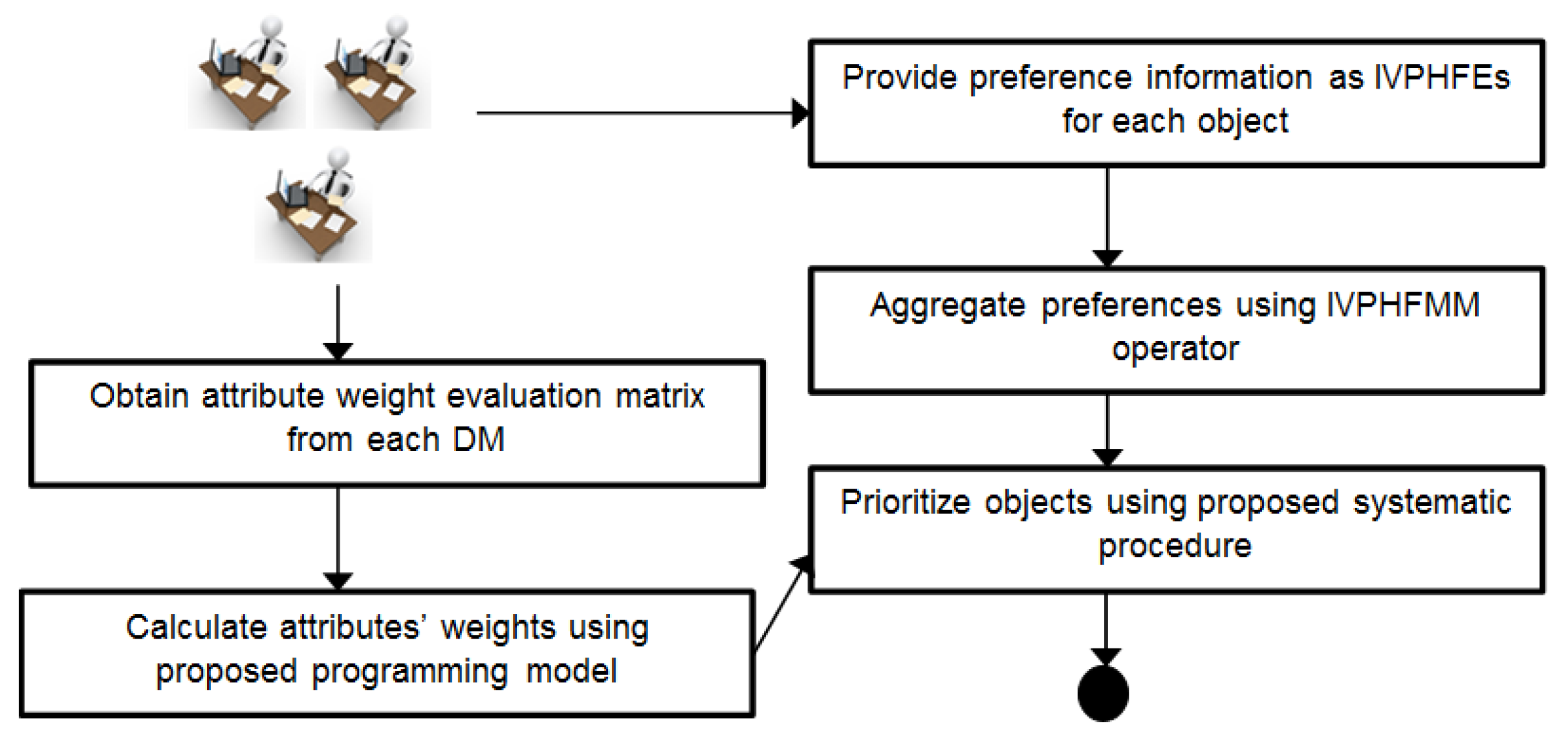
3.3. Proposed MAGDM Method for Prioritization of Objects

This section develops a ranking procedure for prioritizing objects based on the operational laws and newly proposed IVPHFMM operator. The procedure is presented below:

Step 1:

Begin.

Step 2:

Construct $k$ decision matrices of order $m\times n$ where $m$ is the number of objects and $n$ is the number of attributes.

Step 3:

Aggregate these matrices into a single matrix of order $m\times n$ by using newly proposed IVPHFMM operator (see Section 3.1).

Step 4:

Multiply the weight of each attribute with the respective IVPHFE and use Equation (4) attribute-wise to calculate the net value for each object. The resultant value is also an IVPHFE.

Step 5:

Prioritize the objects by adopting transformation method given in Equation (12).

$$h_l^{single}={\displaystyle \sum }_{i=1}^{\#instance}\left(\frac{{\gamma }_i{p}_i^l+{\gamma }_i{p}_i^u}{2}\right)$$

(12)

where $l$ is the index for the object.

Arrange $h_l^{single}$ in the descending order of values to obtain ranking order.

Step 6:

End.

Before demonstrating the practical use of the proposed framework, Figure 1 is presented to obtain a clear view of the implementation process of the proposed framework. Initially, DMs’ preference information is obtained as IVPHFEs for each object over a specific attribute. These matrices are aggregated using newly proposed IVPHFMM operator (refer Section 3.1) which extends the MM operator in the IVPHFS context. An evaluation matrix is obtained from the DMs for attribute weight calculation. Mathematical programming model (refer to Section 3.2) is proposed for calculating the weights of the attributes with the help of partially known information. Finally, a new systematic procedure (refer to Section 3.3) is developed for prioritizing objects which uses the aggregated matrix and weight vector as input for implementation.

4. Numerical Example: Renewable Energy Source Selection from the Indian Perspective

This section demonstrates the practicality of the proposed method by solving renewable energy source selection problem from an Indian perspective which is adapted from Reference [35]. India has a great appetite for energy owing to its high technological advancement and opportunities. Around 85,000 MW of energy demand is potentially satisfied with the help of biomass, small hydro, solar and wind energy. Recently, Mardani et al. [36] conducted a thorough survey of energy source selection using MADM methods and projected the key importance of MADM methods for energy selection. Luthra et al. [37] conducted a deep investigation of barriers to energy sources in India and suggested ideas for the mitigation of challenges from the Indian perspective. In a recent study performed by the Economic Times on energy demand and supply, they predicted that by 2040: (i) there will be a 30% increase in energy which crosses the conventional energy charts and forces an urgent need for renewable energy sources; (ii) also by 2040, India will reach 49% renewable energy usage.

Motivated by the investigation, in this paper, we formulate the renewable source selection problem as an MADM problem and present a systematic procedure for the suitable selection of renewable energy sources.

Step 1:

Construct a panel of three DMs viz., technical personnel $e_1$, member of the ministry of energy and natural resource $e_2$ and senior financial personnel $e_3$. Make an initial list of renewable energy sources and attributes. By systematic pre-screening, the panel finalizes four renewable energy sources and four attributes. These are adapted from Reference [35] and the panel decides to use IVPHFS information for rating energy sources against the attribute.

Step 2:

Form three matrices of order $4\times 4$ where the rows represent the energy sources and columns represent the attributes. Four renewable energy sources considered are geothermal $a_1$, solar $a_2$, tidal $a_3$ and hydro $a_4$ which are evaluated over four attributes viz., technical aspects $c_1$, social aspects $c_2$, financial aspects $c_3$ and environmental aspects $c_4$ IVPHFS information (refer Definition 3) is used for rating energy sources and it is depicted in

Table 2. Interval-valued probabilistic hesitant fuzzy set (IVPHFS) based preference information for different DMs.

Energy	Evaluation Attribute
	c1	c2	c3	c4
$e_1$
$a_1$	$\left\{\begin{array}{c}0.85,\left[0.12,0.12\right]\\ 0.58,\left[0.2,0.48\right]\end{array}\right\}$	$\left\{\begin{array}{c}0.12,\left[0.41,0.41\right]\\ 0.6,\left[0.29,0.29\right]\end{array}\right\}$	$\left\{\begin{array}{c}0.21,\left[0.74 , 0.88 \right]\\ 0.8,\left[ 0.16 , 0.89 \right]\end{array}\right\}$	$\left\{\begin{array}{c}0.79,\left[0.46 , 0.46\right]\\ 0.73,\left[0.34 , 0.83\right]\end{array}\right\}$
$a_2$	$\left\{\begin{array}{c}0.86,\left[0.49,0.57\right]\\ 0.39,\left[0.66,0.66\right]\end{array}\right\}$	$\left\{\begin{array}{c}0.79,\left[0.39,0.39\right]\\ 0.55,\left[0.54,0.54\right]\end{array}\right\}$	$\left\{\begin{array}{c}0.79,\left[0.51 , 0.8\right]\\ 0.39,\left[0.17 , 0.73\right]\end{array}\right\}$	$\left\{\begin{array}{c}0.28,\left[0.25 , 0.3\right]\\ 0.28,\left[0.2 , 0.2\right]\end{array}\right\}$
$a_3$	$\left\{\begin{array}{c}0.21,\left[0.26,0.43\right]\\ 0.81,\left[0.4,0.76\right]\end{array}\right\}$	$\left\{\begin{array}{c}0.63,\left[0.13,0.85\right]\\ 0.31,\left[0.56,0.59\right]\end{array}\right\}$	$\left\{\begin{array}{c}0.29,\left[0.21 , 0.21\right]\\ 0.61,\left[0.75 , 0.84\right]\end{array}\right\}$	$\left\{\begin{array}{c}0.2,\left[0.11 , 0.11\right]\\ 0.71,\left[0.12 , 0.12\right]\end{array}\right\}$
$a_4$	$\left\{\begin{array}{c}0.71,\left[0.32,0.32\right]\\ 0.43,\left[0.65,0.88\right]\end{array}\right\}$	$\left\{\begin{array}{c}0.49,\left[0.35,0.71\right]\\ 0.23,\left[0.2,0.2\right]\end{array}\right\}$	$\left\{\begin{array}{c}0.58,\left[0.64 , 0.64\right]\\ 0.19,\left[0.5 , 0.7\right]\end{array}\right\}$	$\left\{\begin{array}{c}0.28,\left[0.33 , 0.33\right]\\ 0.58,\left[0.28 , 0.43\right]\end{array}\right\}$
$e_2$
$a_1$	$\left\{\begin{array}{c}0.88,\left[0.19,0.19\right]\\ 0.11,\left[0.17,0.71\right]\end{array}\right\}$	$\left\{\begin{array}{c}0.31,\left[0.39,0.39\right]\\ 0.56,\left[0.47,0.84\right]\end{array}\right\}$	$\left\{\begin{array}{c}0.89,\left[0.64 , 0.64\right]\\ 0.1,\left[0.34 , 0.73\right]\end{array}\right\}$	$\left\{\begin{array}{c}0.29,\left[0.1 , 0.11\right]\\ 0.43,\left[0.1 , 0.1\right]\end{array}\right\}$
$a_2$	$\left\{\begin{array}{c}0.24,\left[0.34,0.44\right]\\ 0.53,\left[0.71,0.71\right]\end{array}\right\}$	$\left\{\begin{array}{c}0.54,\left[0.45,0.48\right]\\ 0.8,\left[0.19,0.19s\right]\end{array}\right\}$	$\left\{\begin{array}{c}0.47,\left[0.15 , 0.31\right]\\ 0.79,\left[0.32 , 0.32\right]\end{array}\right\}$	$\left\{\begin{array}{c}0.35,\left[0.35 , 0.35\right]\\ 0.35,\left[0.19 , 0.23\right]\end{array}\right\}$
$a_3$	$\left\{\begin{array}{c}0.65,\left[0.47 , 0.73\right]\\ 0.89,\left[0.13 , 0.77\right]\end{array}\right\}$	$\left\{\begin{array}{c}0.52,\left[0.27 , 0.51\right]\\ 0.39,\left[0.18 , 0.18\right]\end{array}\right\}$	$\left\{\begin{array}{c}0.81,\left[0.34 , 0.57\right]\\ 0.46,\left[0.58 , 0.58\right]\end{array}\right\}$	$\left\{\begin{array}{c}0.4,\left[0.32 , 0.48\right]\\ 0.33,\left[0.19 , 0.23\right]\end{array}\right\}$
$a_4$	$\left\{\begin{array}{c}0.85,\left[0.27 , 0.27\right]\\ 0.89,\left[0.31 , 0.79\right]\end{array}\right\}$	$\left\{\begin{array}{c}0.87,\left[0.27 , 0.27\right]\\ 0.52,\left[0.29 , 0.29\right]\end{array}\right\}$	$\left\{\begin{array}{c}0.28,\left[0.39 , 0.77\right]\\ 0.43,\left[0.3 , 0.3\right]\end{array}\right\}$	$\left\{\begin{array}{c}0.11,\left[0.32 , 0.63\right]\\ 0.32,\left[0.21 , 0.46\right]\end{array}\right\}$
$e_3$
$a_1$	$\left\{\begin{array}{c}0.63,\left[0.2 , 0.2\right]\\ 0.6,\left[0.33 , 0.33\right]\end{array}\right\}$	$\left\{\begin{array}{c}0.54,\left[0.45 , 0.45\right]\\ 0.68,\left[0.15 , 0.15\right]\end{array}\right\}$	$\left\{\begin{array}{c}0.85,\left[0.52 , 0.52\right]\\ 0.8,\left[0.11 , 0.11\right]\end{array}\right\}$	$\left\{\begin{array}{c}0.48,\left[0.21 , 0.22\right]\\ 0.58,\left[0.22 , 0.29\right]\end{array}\right\}$
$a_2$	$\left\{\begin{array}{c}0.56,\left[0.15 , 0.15\right]\\ 0.57,\left[0.65 , 0.7\right]\end{array}\right\}$	$\left\{\begin{array}{c}0.78,\left[0.57 , 0.57\right]\\ \{0.48,\left[0.19 , 0.29\right]\end{array}\right\}$	$\left\{\begin{array}{c}0.24,\left[0.63 , 0.63\right]\\ 0.57,\left[0.38 , 0.38\right]\end{array}\right\}$	$\left\{\begin{array}{c}0.29,\left[0.31 , 0.33\right]\\ 0.33,\left[0.22 , 0.24\right]\end{array}\right\}$
$a_3$	$\left\{\begin{array}{c}0.53,\left[0.44 , 0.44\right]\\ 0.16,\left[0.33 , 0.33\right]\end{array}\right\}$	$\left\{\begin{array}{c}0.84,\left[0.13 , 0.38\right]\\ 0.78,\left[0.43 , 0.63\right]\end{array}\right\}$	$\left\{\begin{array}{c}0.15,\left[0.2 , 0.86\right]\\ 0.34,\left[0.35 , 0.35\right]\end{array}\right\}$	$\left\{\begin{array}{c}0.34,\left[0.22 , 0.34\right]\\ 0.31,\left[0.22 , 0.25\right]\end{array}\right\}$
$a_4$	$\left\{\begin{array}{c}0.46,\left[0.83 , 0.83\right]\\ 0.64,\left[0.33 , 0.33\right]\end{array}\right\}$	$\left\{\begin{array}{c}0.2,\left[0.54 , 0.54\right]\\ 0.82,\left[0.41 , 0.41\right]\end{array}\right\}$	$\left\{\begin{array}{c}0.84,\left[0.25 , 0.25\right]\\ 0.69,\left[0.23 , 0.37\right]\end{array}\right\}$	$\left\{\begin{array}{c}0.21,\left[0.31 , 0.54\right]\\ 0.51,\left[0.27 , 0.42\right]\end{array}\right\}$

.

Table 2 presents the preference information by different DMs over renewable energy sources based on a set of attributes. IVPHFS based preference information is adopted.

Step 3:

Aggregate the IVPHFEs from Table 2 by using IVPHFMM operator (see Section 3.1 for details). There are three risk appetite values used viz., ${\lambda }_1$, ${\lambda }_2$ and ${\lambda }_3$ which are given by 2, 2 and 1. The weight of each DM is given by 0.3, 0.4 and 0.3.

The preference information from Table 2 is aggregated using IVPHFMM operator and it is shown in

Table 3. Aggregation of preferences by using interval-valued probabilistic hesitant fuzzy Muirhead mean (IVPHFMM) operator.

Energy	Evaluation Attribute
	${\mathit{c}}_1$	${\mathit{c}}_2$	${\mathit{c}}_3$	${\mathit{c}}_4$
$e_{123}$
$a_1$	$\left\{\begin{array}{c} 0.79, \left[ 0.17 , 0.17 \right]\\ 0.3, \left[ 0.22 , 0.5 \right]\end{array}\right\}$	$\left\{\begin{array}{c} 0.27, \left[ 0.41 , 0.41\right]\\ 0.61, \left[ 0.29 , 0.37 \right]\end{array}\right\}$	$\left\{\begin{array}{c} 0.57, \left[ 0.63 , 0.66 \right]\\ 0.35, \left[ 0.19 , 0.44 \right]\end{array}\right\}$	$\left\{\begin{array}{c}0.48, \left[ 0.21 , 0.22 \right]\\ 0.58, \left[ 0.22 , 0.29 \right]\end{array}\right\}$
$a_2$	$\left\{\begin{array}{c} 0.46, \left[ 0.3 , 0.34 \right]\\ 0.5, \left[ 0.68 , 0.69\right]\end{array}\right\}$	$\left\{\begin{array}{c} 0.67, \left[ 0.46 , 0.47 \right]\\ 0.61, \left[ 0.26 , 0.3 \right]\end{array}\right\}$	$\left\{\begin{array}{c} 0.45, \left[ 0.34 , 0.51 \right]\\ 0.58, \left[ 0.28 , 0.43 \right]\end{array}\right\}$	$\left\{\begin{array}{c} 0.29, \left[ 0.31 , 0.33 \right]\\ 0.33, \left[ 0.22 , 0.24 \right]\end{array}\right\}$
$a_3$	$\left\{\begin{array}{c} 0.43, \left[ 0.39 , 0.54 \right]\\ 0.51, \left[ 0.24 , 0.6 \right]\end{array}\right\}$	$\left\{\begin{array}{c} 0.64, \left[ 0.17 , 0.54 \right]\\ 0.45, \left[ 0.33 , 0.37\right]\end{array}\right\}$	$\left\{\begin{array}{c} 0.36, \left[ 0.25 , 0.48 \right]\\ 0.45, [ 0.54 , 0.56 \end{array}\right\}$	$\left\{\begin{array}{c} 0.34, \left[ 0.22 , 0.34\right]\\ 0.31, \left[ 0.22 , 0.25 \right]\end{array}\right\}$
$a_4$	$\left\{\begin{array}{c}0.67, \left[ 0.4 , 0.4 \right]\\ 0.49, \left[ 0.39 , 0.63 \right]\end{array}\right\}$	$\left\{\begin{array}{c} 0.47, \left[ 0.36 , 0.45 \right]\\ 0.47, \left[ 0.29 , 0.29 \right]\end{array}\right\}$	$\left\{\begin{array}{c} 0.48, \left[ 0.4 , 0.52 \right]\\ 0.39, [ 0.32 , 0.41 \end{array}\right\}$	$\left\{\begin{array}{c} 0.21, \left[ 0.31 , 0.54 \right]\\ 0.51, \left[ 0.27 , 0.42 \right]\end{array}\right\}$

. Clearly, from Table 3, we can observe that the aggregated value is also an IVPHFE (refer Definition 3).

Step 4:

Calculate the weights of the attributes by using the procedure given in Section 3.2.

Table 4. Evaluation matrix for attribute weight calculation.

DMs	Evaluation Attribute
	${\mathit{c}}_1$	${\mathit{c}}_2$	${\mathit{c}}_3$	${\mathit{c}}_4$
$e_1$	$\left\{\begin{array}{c}0.5,\left[0.5,0.7\right]\\ 0.4,\left[0.35,0.45\right]\end{array}\right\}$	$\left\{\begin{array}{c}0.44,\left[0.45,0.5\right]\\ 0.54,\left[0.5,0.6\right]\end{array}\right\}$	$\left\{\begin{array}{c}0.55,\left[0.55,0.65\right]\\ 0.45,\left[0.55,0.7\right]\end{array}\right\}$	$\left\{\begin{array}{c}0.65,\left[0.35,0.4\right]\\ 0.4,\left[0.4,0.45\right]\end{array}\right\}$
$e_2$	$\left\{\begin{array}{c}0.6,\left[0.6,0.65\right]\\ 0.45,\left[0.45,0.5\right]\end{array}\right\}$	$\left\{\begin{array}{c}0.35,\left[0.6,0.7\right]\\ 0.5,\left[0.55,0.65\right]\end{array}\right\}$	$\left\{\begin{array}{c}0.45,\left[0.54,0.65\right]\\ 0.35,\left[0.4,0.6\right]\end{array}\right\}$	$\left\{\begin{array}{c}0.55,\left[0.5,0.7\right]\\ 0.4,\left[0.6,0.7\right]\end{array}\right\}$
$e_3$	$\left\{\begin{array}{c}0.45,\left[0.5,0.6\right]\\ 0.4,\left[0.55,0.65\right]\end{array}\right\}$	$\left\{\begin{array}{c}0.4\left[0.5,0.6\right]\\ 0.5,\left[0.4,0.55\right]\end{array}\right\}$	$\left\{\begin{array}{c}0.45,\left[0.45,0.55\right]\\ 0.6,\left[0.35,0.55\right]\end{array}\right\}$	$\left\{\begin{array}{c}0.45,\left[0.55,0.65\right]\\ 0.6,\left[0.6,0.65\right]\end{array}\right\}$

shows an evaluation matrix with IVPHFS information which is used to calculate the PIS and NIS values for each attribute (see Table 4).

By using Table 4 and

Table 5. PIS & NIS for each attribute.

Ideal Solution	Evaluation Attribute
	${\mathit{c}}_1$	${\mathit{c}}_2$	${\mathit{c}}_3$	${\mathit{c}}_4$
$h^{+}$	$\left\{\begin{array}{c} 0.6, \left[0.6,0.65\right]\\ 0.45, \left[0.45,0.5\right]\end{array}\right\}$	$\left\{\begin{array}{c} 0.35, \left[0.6,0.7\right]\\ 0.5, \left[0.55,0.65\right]\end{array}\right\}$	$\left\{\begin{array}{c} 0.45, \left[0.54,0.65\right]\\ 0.35, \left[0.4,0.6\right]\end{array}\right\}$	$\left\{\begin{array}{c} 0.45, \left[0.55,0.65\right]\\ 0.6, \left[0.6,0.65\right]\end{array}\right\}$
$h^{-}$	$\left\{\begin{array}{c} 0.5, \left[0.5,0.7\right]\\ 0.4, \left[0.35,0.45\right]\end{array}\right\}$	$\left\{\begin{array}{c} 0.4, \left[0.5,0.6\right]\\ 0.5, \left[0.4,0.55\right]\end{array}\right\}$	$\left\{\begin{array}{c} 0.55, \left[0.55,0.65\right]\\ 0.45, \left[0.55,0.7\right]\end{array}\right\}$	$\left\{\begin{array}{c}0.65, \left[0.35,0.4\right]\\ 0.4, \left[0.4,0.45\right]\end{array}\right\}$

the objective function is constructed from Model 1. The constraints are obtained from the DMs and the model is solved using optimization toolbox of MATLAB®. From Model 1, we get the objective function as $MinZ=0.38w_1-0.008w_2-0.043w_3+0.112w_4$ and the inequality constraints are given by $w_1\le 0.3$, $w_2\le 0.3$, $w_3\le 0.3$ and $w_4\le 0.3$. By solving we get, $w_1=w_2=w_3=0.3$ and $,w_4=0.1$.

Step 5:

Prioritize the energy sources by using the procedure given in Section 3.3.

The cumulative ring sum value for each renewable energy source is given by $\begin{array}{c}0.97,\left[0.86,0.87\right],0.93,\left[0.65,0.87\right];0.93,\left[0.83,0.89\right],0.95,\left[0.87,0.91\right];\\ 0.91,\left[0.7,0.93\right],0.9,\left[0.82,0.92\right];0.93,\left[0.84,0.93\right],0.92,\left[0.79,0.91\right]\end{array}$ for unbiased attributes’ weights and $\begin{array}{c}0.41,\left[0.33,0.34\right],0.34,\left[0.20,0.33\right];0.37,\left[0.29,0.34\right],0.39,\left[0.31,0.35\right];\\ 0.34,\left[0.23,0.37\right],0.34,\left[0.30,0.37\right];0.37,\left[0.30,0.36\right],0.34,\left[0.27,0.34\right]\end{array}$ for biased attributes’ weights. From Equation (12) we get, $a_1=1.54$, $a_2=1.63$, $a_3=1.52$ and $a_4=1.6$ for unbiased weight values and $a_1=0.23$, $a_2=0.25$, $a_3=0.23$ and $a_4=0.23$ for biased weight values. Thus, the ranking order is $a_2\succ a_4\succ a_1\succ a_3$ and the suitable renewable energy source for the process is solar energy $a_2$.

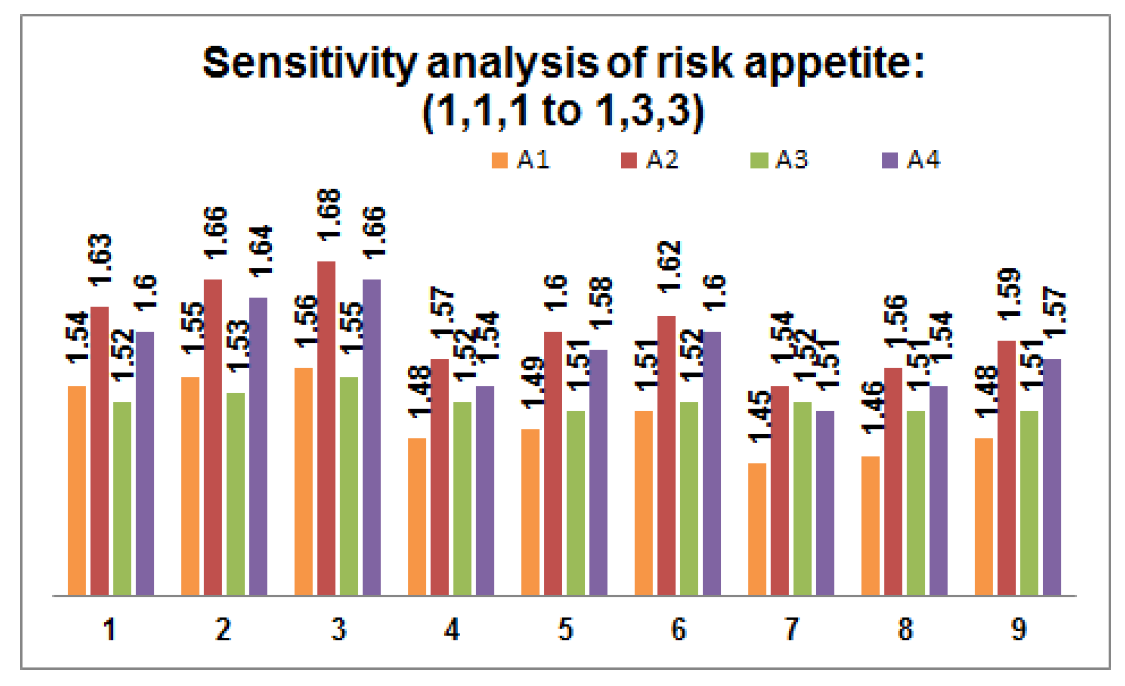
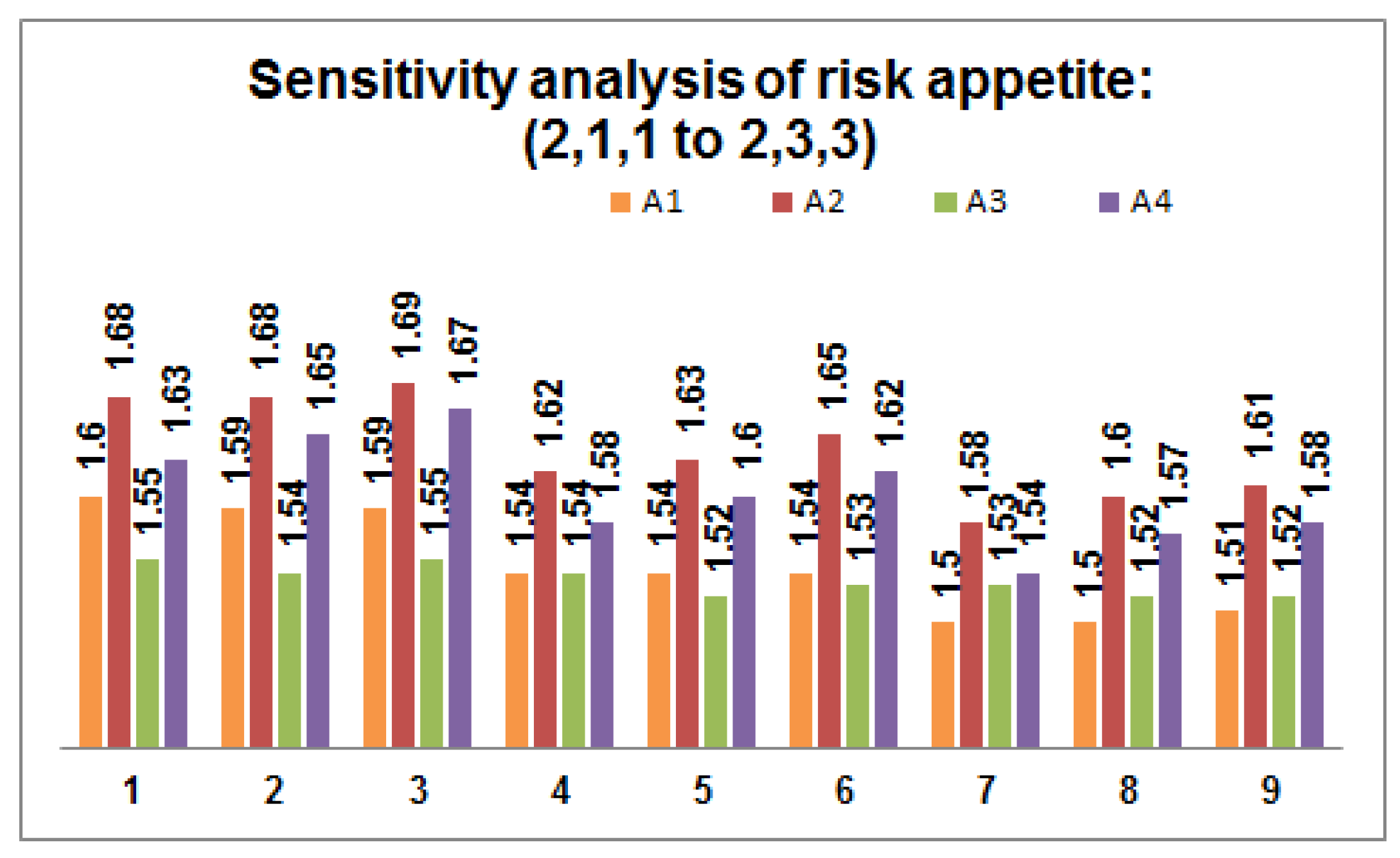
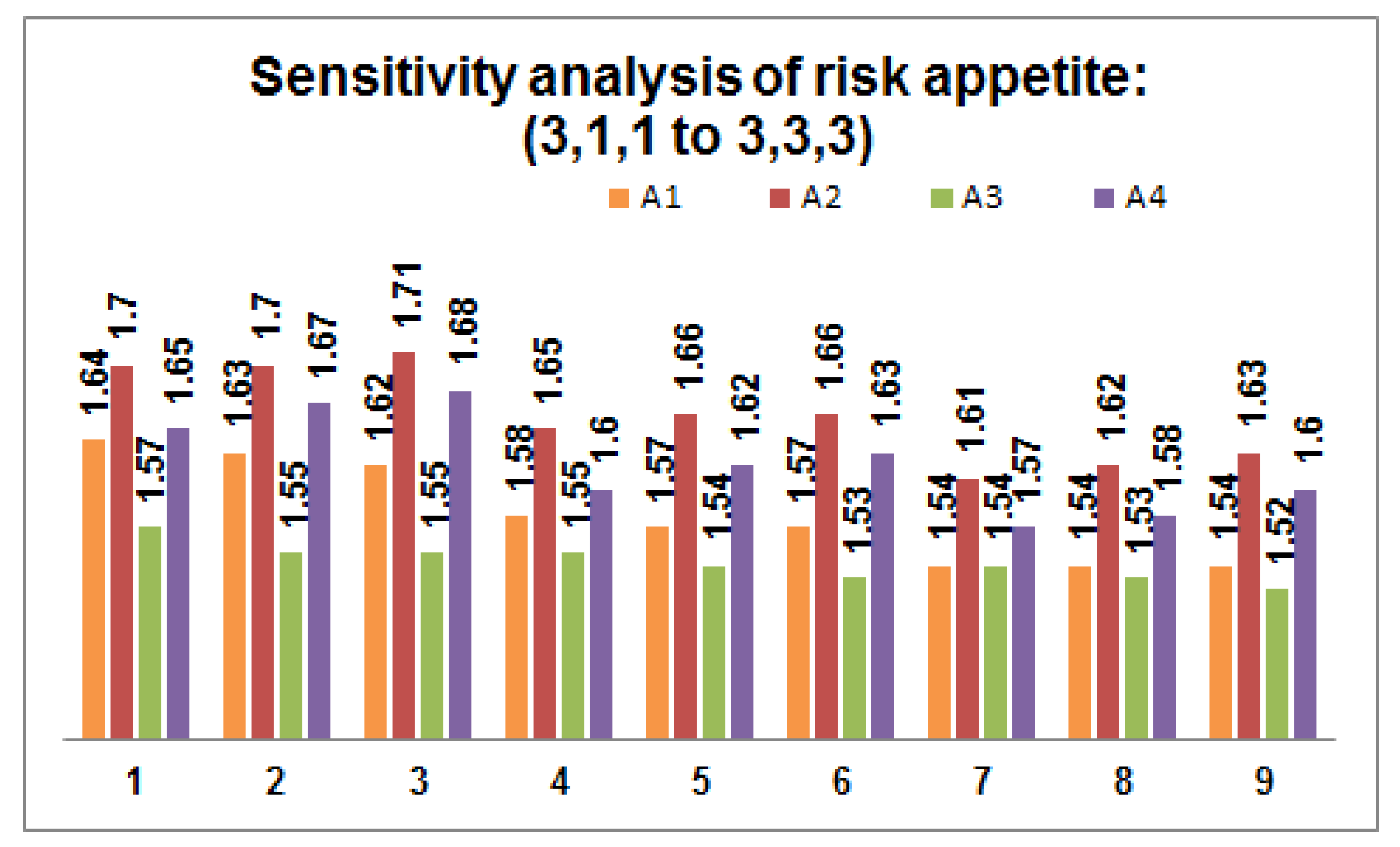
Step 6:

Perform sensitivity analysis on the risk appetite of each DM by varying the values within the predefined threshold value. Figure 2, Figure 3 and Figure 4 depict 27 possible risk appetite values and the corresponding prioritized value for each renewable energy source. From the analysis, we can clearly observe that the prioritized order remains unchanged with the final order as $a_2\succ a_4\succcurlyeq a_1\succ a_3$ with solar energy as a suitable renewable energy source for the process taken into consideration.

Step 7:

End.

5. Comparative Analysis of Proposed Decision Framework

This section put forwards a comparative study of the proposed aggregation operator with other operators in the IVPHFS context. In order to maintain the homogeneity of the comparison process, we analyse the proposed method with aggregation operators from References [18] and [19] which uses IVPHFEs as preference information.

Table 6. The ranking order of renewable energy sources: Proposed vs. Others.

Methods	Renewable Energy Source (s)				Order
	a1	a2	a3	a4
[18]	2	1	4	3	$a_2\succ a_1\succ a_4\succ a_3$
[19]	2	1	4	3	$a_2\succ a_1\succ a_4\succ a_3$
Proposed	3	1	4	2	$a_2\succ a_4\succ a_1\succ a_3$

Note: DMs’ weight values are considered as 0.3, 0.4 and 0.3 respectively and the attributes’ weight values are considered as 0.25.

depicts the ranking order from different methods and we can see that the proposed method produces a unique ranking order compared to its counterpart. This is mainly due to the ability of the proposed aggregation operator to capture the interrelationship between multiple attributes. The consistency of the proposed method is realized by calculating the Spearman correlation coefficient [38] for each method. Figure 5 depicts the correlation plot for each method and we can infer that the proposed method is highly consistent with other state-of-the-art methods.

Table 7. Characteristics analysis for proposed vs. other methods.

Characteristics	Methods
	Proposed	[18]	[19]
Data	IVPHFS based preference information
Comprehensive data	yes	yes	yes
Interrelationship	yes	no	no
Customizable parameter(s)	yes	no	no
Total pre-order	yes	yes	yes
Generalizability	yes	no	no
The relative importance of DM	yes	yes	yes
Risk appetite of DM	yes	no	no
Information loss	Mitigated in an efficient manner	Mitigated in a moderate manner

depicts the characteristics analysis of different methods. The characteristics are adapted from the work of Liu and Teng [32].

Some strengths of the proposed method are listed below:

• The proposed aggregation operator uses the generalized data structure viz., IVPHFS as preference information. The interval number is associated as an occurrence probability value for each HFE.
• The extension of MM operator to IVPHFS context provides DMs with the ability to capture interrelationship between multiple attributes. This property resembles closely with the real-life decision-making problem.
• The proposed operator not only obtains weights of DMs but also considers the risk appetite of each DM.
• The proposed operator has parameters that are easily customizable for realizing different effects on prioritization of objects.
• The proposed operator can also realize certain operators as special cases which provide a generalized context for aggregation of preferences that helps DMs is effective management of uncertainty and vagueness.
• The attributes’ weight values are calculated in a rational manner by considering the partial information from each DM.

Some weaknesses of the proposed method are:

• It is difficult to fix the parameter value for different MAGDM application without a trial and error process.
• DMs need some training with the data structure for proper elicitation of preferences.

6. Conclusions

This paper presents a new extension to MM operator in the IVPHFS context. Some interesting properties and theorems are also discussed for arriving better theoretical perspective in the field of aggregation and information fusion. The weights of the attributes are also calculated using newly proposed mathematical programming model which uses the DMs’ partial information effectively. The data structure used for preference elicitation is a generalization of PHFS concept that mitigates the problem of assigning a precise occurrence probability to each HFE by allowing interval values as occurrence probability for each HFE. The MM operator has the ability to capture interrelationship between multiple attributes and provides a generalized focus on the aggregation of preferences. The customizable parameter in MM operator allows DMs to clearly understand the effect of risk appetite value on the prioritization order. The idea of extending the MM operator to IVPHFS context and the proposing of a new programming model for attribute weight calculation enriches the data structure for better MAGDM. Some desirable properties of the proposed IVPHFMM operator have analyzed for better understanding the operator and applying the same for MAGDM. From the sensitivity analysis of risk appetite values, we can infer that as values increase, the rank values also increase for each renewable energy source, thus allowing rational prioritization of renewable energy sources. Also, sensitivity analysis is carried out for attribute weight values and they infer that the prioritization order is unchanged and the proposed prioritization procedure is stable even after adequate changes are made to the attributes’ weights.

As a part of the future direction, plans are made to extend different generalized operators in the IVPHFS context with a discussion on different Archimedean T-norms and T-conorms. Further, plans are made to propose a new decision framework in the IVPHFS context for better MAGDM and large scale group decision-making.

References

- Triantaphyllou, E.; Shu, B. Multi-criteria decision making: An operations research approach. Encycl. Electr. Electron. Eng. 1998, 15, 175–186. [Google Scholar]
- Torra, V. Hesitant fuzzy sets. Int. J. Intell. Syst. 2010, 25, 529–539. [Google Scholar] [CrossRef]
- Zadeh, L.A. Fuzzy sets. Inf. Control 1965, 8, 338–353. [Google Scholar] [CrossRef]
- Chai, J.; Ngai, E.W.T. Multi-perspective strategic supplier selection in uncertain environments. Int. J. Prod. Econ. 2015, 166, 215–225. [Google Scholar] [CrossRef]
- Krishankumar, R.; Ravichandran, K.S.; Murthy, K.K.; Saeid, A.B. A scientific decision-making framework for supplier outsourcing using hesitant fuzzy information. Soft Comput. 2018, 22, 7445–7461. [Google Scholar] [CrossRef]
- Aktas, A.; Kabak, M. A hybrid hesitant fuzzy decision-making approach for evaluating solar power plant location sites. Arab. J. Sci. Eng. 2018, 1–13. [Google Scholar] [CrossRef]
- Senvar, O.; Otay, I.; Bolturk, E. Hospital site selection via hesitant fuzzy TOPSIS. IFAC-PapersOnLine 2016, 49, 1140–1145. [Google Scholar] [CrossRef]
- Zhang, F.; Chen, J.; Zhu, Y.; Li, J.; Li, Q.; Zhuang, Z. A dual hesitant fuzzy rough pattern recognition approach based on deviation theories and its application in urban traffic modes recognition. Symmetry. 2017, 9, 262. [Google Scholar] [CrossRef]
- Rodríguez, R.M.; Martínez, L.; Torra, V.; Xu, Z.S.; Herrera, F. Hesitant fuzzy sets: State of the art and future directions. Int. J. Intell. Syst. 2014, 29, 495–524. [Google Scholar] [CrossRef]
- Xu, Z.S.; Zhou, W. Consensus building with a group of decision makers under the hesitant probabilistic fuzzy environment. Fuzzy Optim. Decis. Mak. 2016, 16, 1–23. [Google Scholar] [CrossRef]
- Yue, L.; Sun, M.; Shao, Z. The probabilistic hesitant fuzzy weighted average operators and their application in strategic decision making. J. Inf. Comput. Sci. 2013, 10, 3841–3848. [Google Scholar] [CrossRef]
- Li, J.; Wang, Z. Multi-attribute decision making based on prioritized operators under probabilistic hesitant fuzzy environments. Soft Comput. 2018, 1–16. [Google Scholar] [CrossRef]
- Hao, Z.; Xu, Z.S.; Zhao, H.; Su, Z. Probabilistic dual hesitant fuzzy set and its application in risk evaluation. Knowledge-Based Syst. 2017, 127, 16–28. [Google Scholar] [CrossRef]
- Zhou, W.; Xu, Z.S. Group consistency and group decision making under uncertain probabilistic hesitant fuzzy preference environment. Inf. Sci. 2017, 414, 276–288. [Google Scholar] [CrossRef]
- Bashir, Z.; Rashid, T.; Watróbski, J.; Salabun, W.; Malik, A. Hesitant probabilistic multiplicative preference relations in group decision making. Appl. Sci. 2018, 8, 3998. [Google Scholar] [CrossRef]
- Gao, J.; Xu, Z.S.; Liao, H. A dynamic reference point method for emergency response under hesitant probabilistic fuzzy environment. Int. J. Fuzzy Syst. 2017, 19, 1261–1278. [Google Scholar] [CrossRef]
- Jiang, F.; Ma, Q. Multi-attribute group decision making under probabilistic hesitant fuzzy environment with application to evaluate the transformation efficiency. Appl. Intell. 2017, 48, 953–965. [Google Scholar] [CrossRef]
- Song, C.; Zhao, H.; Xu, Z.S.; Hao, Z. Interval-valued probabilistic hesitant fuzzy set and its application in the Arctic geopolitical risk evaluation. Int. J. Intell. Syst. 2018, 1–25. [Google Scholar] [CrossRef]
- Krishankumar, R.; Ravichandran, K.S.; Kar, S.; Gupta, P.; Mehlawat, M.K. Interval-valued probabilistic hesitant fuzzy set for multi-criteria group decision-making. Soft Comput. 2018, 1–27. [Google Scholar] [CrossRef]
- Moscovici, S.; Zavalloni, M. The group as a polarizer of attitudes. J. Pers. Soc. Psychol. 1969, 12, 125–135. [Google Scholar] [CrossRef]
- Mesiar, R.; Calvo, T. Fuzzy sets and their extensions: Representation, aggregation and models. Stud. Fuzziness Soft Comput. 2008, 220, 1–22. [Google Scholar]
- Muirhead, R.F. Some methods applicable to identities and inequalities of symmetric algebraic functions of n letters. Proc. Edinburgh Math. Soc. 1902, 21, 144–162. [Google Scholar] [CrossRef]
- Xia, M.; Xu, Z.S.; Zhu, B. Geometric Bonferroni means with their application in multi-criteria decision making. Knowledge-Based Syst. 2013, 40, 88–100. [Google Scholar] [CrossRef]
- Qin, J.; Liu, X.; Pedrycz, W. Hesitant fuzzy Maclaurin symmetric mean operators and its application to multiple-attribute decision making. Int. J. Fuzzy Syst. 2015, 17, 509–520. [Google Scholar] [CrossRef]
- Wang, R.; Wang, J.; Gao, H.; Wei, G. Methods for MADM with picture fuzzy Muirhead mean operators and their application for evaluating the financial investment risk. Symmetry 2019, 11, 6. [Google Scholar] [CrossRef]
- Liu, P.; Khan, Q.; Mahmood, T.; Hassan, N. T-spherical fuzzy power Muirhead mean operator based on novel operational laws and their application in multi-attribute group decision making. IEEE Access 2019, 7, 22613–22632. [Google Scholar] [CrossRef]
- Liu, P.; Li, Y.; Zhang, M.; Zhang, L.; Zhao, J. Multiple-attribute decision-making method based on hesitant fuzzy linguistic Muirhead mean aggregation operators. Soft Comput. 2018, 22, 5513–5524. [Google Scholar] [CrossRef]
- Hong, Z.; Rong, Y.; Qin, Y.; Liu, Y. Hesitant fuzzy dual Muirhead mean operators and its application to multiple attribute decision making. J. Intell. Fuzzy Syst. 2018, 35, 2161–2172. [Google Scholar] [CrossRef]
- Khan, Q.; Hassan, N.; Mahmood, T. Neutrosophic cubic power Muirhead mean operators with uncertain data for multi-attribute decision-making. Symmetry 2018, 10, 444. [Google Scholar] [CrossRef]
- Xu, Y.; Shang, X.; Wang, J. Pythagorean fuzzy interaction Muirhead means with their application to multi-attribute group decision-making. Inf. 2018, 9, 157. [Google Scholar] [CrossRef]
- Wang, J.; Zhang, R.; Zhu, X.; Zhou, Z.; Shang, X.; Li, W. Some q-rung orthopair fuzzy Muirhead means with their application to multi-attribute group decision-making. J. Intell. Fuzzy Syst. 2018, 36, 1–19. [Google Scholar] [CrossRef]
- Liu, P.; Teng, F. Some Muirhead mean operators for probabilistic linguistic term sets and their applications to multiple attribute decision-making. Appl. Soft Comput. 2018, 68, 396–431. [Google Scholar] [CrossRef]
- Saaty, T.L. Decision making with the analytic hierarchy process. Int. J. Serv. Sci. 2008, 1, 83. [Google Scholar] [CrossRef]
- Gupta, P.; Mehlawat, M.K.; Grover, N. Intuitionistic fuzzy multi-attribute group decision-making with an application to plant location selection based on a new extended VIKOR method. Inf. Sci. 2016, 370, 184–203. [Google Scholar] [CrossRef]
- Chatterjee, K.; Kar, S. A multi-criteria decision making for renewable energy selection using Z-numbers. Technol. Econ. Dev. Econ. 2018, 24, 739–764. [Google Scholar] [CrossRef]
- Mardani, A.; Zavadskas, E.K.; Khalifah, Z.; Zakuan, N.; Jusoh, A.; Nor, K.M.; Khoshnoudi, M. A review of multi-criteria decision-making applications to solve energy management problems: Two decades from 1995 to 2015. Renew. Sustain. Energy Rev. 2017, 71, 216–256. [Google Scholar] [CrossRef]
- Luthra, S.; Kumar, S.; Garg, D.; Haleem, A. Barriers to renewable/sustainable energy technologies adoption: Indian perspective. Renew. Sustain. Energy Rev. 2015, 41, 762–776. [Google Scholar] [CrossRef]
- Spearman, C. The proof and measurement of association between two things. Am. J. Psychol. 1904, 15, 72–101. [Google Scholar] [CrossRef]