Abstract
In this paper, the multiblock mortar mixed approximation of second order parabolic partial differential equations is considered. In this method, the simulation domain is decomposed into the non-overlapping subdomains (blocks), and a physically-meaningful boundary condition is set on the mortar interface between the blocks. The governing equations hold locally on each subdomain region. The local problems on blocks are coupled by introducing a special approximation space on the interfaces of neighboring subdomains. Each block is locally covered by an independent grid and the standard mixed finite element method is applied to solve the local problem. The unique solvability of the discrete problem is shown, and optimal order convergence rates are established for the approximate velocity and pressure on the subdomain. Furthermore, an error estimate for the interface pressure in mortar space is presented. The numerical experiments are presented to validate the efficiency of the method.
1. Introduction
The numerical approximation of partial differential equations has received considerable attention due to its applications in diverse fields of science and technology. In modern scientific computation, efficiency and accuracy are the main objectives of numerical methods. Generally, numerical methods reduce the solution of partial differential equations into the solution of an algebraic system of equations. In practical applications, using direct methods, it is very complicated to attain both efficiency and accuracy at the same time. For example, fluid flow in an underground reservoir involves a highly heterogeneous medium. Furthermore, the physical properties of the media change rapidly on a large domain; for example, in fluid flow in porous media, the permeability of fluid fluctuates rapidly. In such cases, either accuracy is sacrificed or a very fine mesh is used to resolve heterogeneity in permeability. The latter gives rise to a huge system of coupled equations, which in many cases becomes very challenging to solve computationally. These difficulties motivated discovering alternate techniques that keep the computational burden manageable along with the maximum possible accuracy.
Several domain decomposition methods have been developed to overcome these difficulties. The purpose of all domain decomposition methods is to provide efficient approximation by alleviating the computation burden. This is achieved by splitting the physical problem into smaller subproblems by dividing the domain into a series of subdomains. This technique allows considering different physical models in different regions. It is also capable of employing the most suitable approximation method in different blocks of the computational domain. We consider the second order linear parabolic partial differential equation modeling single-phase Darcy flow in a porous medium written as a system of first order equations:
where , or 3, and . Equation (1) is the Darcy law, and (2) is the mass conservation. The unknown represents Darcy velocity, and p is the pressure. Assume that a has the continuous bounded derivative up to order two and there exist constants and such that:
Moreover, assume that there exist constants and such that:
Mixed finite element methods have emerged with considerable popularity in several areas of science and engineering. The mixed methods enjoy local mass conservation and provide accurate approximation of two variables of physical interest simultaneously, for example velocity and pressure in fluid flow. They are also capable of approximating both variables with the same accuracy. The mixed finite element methods have been extensively used to solve the elliptic [1,2,3,4,5,6,7,8,9,10,11,12,13,14] and parabolic [15,16,17,18,19] partial differential equations. The mixed finite element methods are also used to approximate the partial differential equations governing fluid flow [20,21,22,23,24,25,26,27,28].
The mortar finite element method was first introduced in [29] for the elliptic partial differential equation. It is a nonconforming domain decomposition method in which the weak continuity condition is imposed across the subdomain interfaces. The mixed finite element method on locally-nested refined grids was developed in [30,31]. In this technique, the continuity of flux across the subdomain block interface is enforced by using the concept of slave or worker nodes. Since in this approach, the grids must be nested, it cannot be extended to the non-matching ones.
The mixed version of the mortar method is proposed and analyzed in [20]. The idea was to divide the original domain into smaller blocks and impose the governing partial differential equation on each block. An unknown pressure is introduced on the interfaces between the subdomains known as the Lagrange multiplier. This new variable provides the Dirichlet boundary condition for the local problem on each subdomain block. This procedure splits the large problem into a series of small subproblems. As a result, the local small-sized problems can be solved more comfortably as compared to a single large problem on the entire domain. This method gives better approximation on non-matching grids. Since different grids are used on the adjacent subdomains, the normal trace of the velocity space cannot be used as a Lagrange multiplier space; therefore, a different space, namely the mortar finite element space, is defined on the inter-block boundaries. The method gives the optimal order convergence if the mortar space approximation is one order higher than the normal trace of the subdomain velocity space. The multiblock approach provides the independent partition of each subdomain block so that an appropriate approximation method can be applied to solve the local problem. This approach offers great flexibility to formulate the different physical and mathematical models on different subdomain blocks. Moreover, the non-overlapping domain decomposition algorithms can be applied to implement the scheme in parallel. The multiblock technique has been further explored to solve several problems, for example [32,33,34].
To the best of the authors’ knowledge, there is no article in the literature that presents a complete analysis of the multiblock mortar mixed approach for the time-dependent problem under consideration. The present study is an extension of the results established in [20] to the parabolic equations. The continuous time discretization is considered, and the difficulties arising in the multiblock mortar mixed formulation of time-dependent problems are addressed. First, the existence and uniqueness of the discrete solution is accomplished by using the established theory for ordinary differential equations. Second, the convergence analysis of parabolic problems requires the construction of elliptic projection [35], which maps the continuous solution into the discrete space. The a priori error estimate is derived via mixed elliptic projection for the approximate velocity and pressure on the subdomain. The error estimate for the unknown mortar pressure through the interface bilinear form as described in [20] is not applicable in our case. Therefore, an alternate way is used, and an error bound for the Lagrange multiplier serving as the Dirichlet boundary condition on mortar the interface is proven. The error estimate for the mortar interface variable predicts the accuracy of data flow across the subdomain interface.
Consider the domain , and let us denote by the boundary of . Let denote the unit outward normal to . Throughout the article, we shall use to denote the or the inner product on . Furthermore the inner product on is denoted by . The or norm will be denoted by . For any non-negative integer ℓ and , let denote the standard Sobolev space. The norm and semi-norm on are denoted by and , respectively. In particular, for denotes the space of ℓ times differentiable functions. The norm on is denoted by In the notation below, we shall omit the subscript when . Throughout the article, the boldface letters are used to denote the vectors. Furthermore, for the weak formulation of mixed finite element methods, the usual function space is defined as:
Finally, for a given norm space equipped with the norm , the function space denotes the space of functions equipped with the norm, for :
and if , the integral is replaced by an essential supremum.
The remainder of the article is outlined as follows. In the next section, we discuss the domain decomposition and the method formulation and present the unique solvability of the discrete problem. The mixed method elliptic projection and related error estimates are given in Section 3. In Section 4, we provide optimal order convergence results. Section 5 deals with the error estimates for unknown mortar. The numerical experiments are provided in Section 6. Finally, the paper is concluded in Section 7.
2. Domain Decomposition and Method Formulation
Let us consider the non-overlapping decomposition of the domain into the series of subdomains such that:
Let us define the interfaces:
Here, denotes the interface between two subdomains, represents the interior skeleton of decomposition, and is the interface related to a single subdomain in the decomposition.
We now define the function spaces to formulate the weak and discrete problems. Let us define the local weak spaces as Then, their global counterparts are given by:
In order to define the discrete finite element spaces, we first partition each subdomain into the local conforming and quasi-uniform mesh denoted by , that is , where E denotes an element in the mesh with maximum diameter . For the purpose of analysis, we define . We allow the possibility that the local grids and on adjacent subdomains and do not necessarily align on the interface. Let us denote by the union of partitions on subdomains , , that is Let us consider the mixed finite element spaces of order . These mixed finite element spaces can be either Raviart–Thomas () [12], or Brezzi–Douglas–Fortin–Marini () [2], or Brezzi–Douglas–Fortin () [1]. Moreover, we assume that the order of approximation is the same on each subdomain. It is well known that the property holds in standard mixed finite element spaces. Then, the corresponding global mixed spaces on are defined by:
Note that the normal components of vectors in the space are continuous between the elements of local grid on each subdomain block , but not across the interface .
We consider the quasi-uniform mesh on mortar interface , denoted by . This mortar interface mesh will be used to define a finite element space that provides the approximation for the Dirichlet boundary condition assigned to the mortar interface. Let us denote by , the mortar space consisting either of continuous or discontinuous piecewise polynomials of degree on the interface mesh, where k is associated with the degree of polynomial in . Note that for and the lowest order Raviart–Thomas space , the mortar space contains piecewise linear polynomials. In the case of and , the mortar space consists of a bilinear polynomial on the interface. Then, the global mortar space on is given by:
In the following, we treat any function as extended by zero on . Also in the case of discontinuous space, need not to be conforming.
A unique solution for the discrete problem exists, if the following technical condition holds.
Assumption 1.
Let be the - orthogonal projection on each subdomain , , satisfying:
then assume that there exists a constant C, independent of h, such that for all :
The condition (7) enforces a limit on the mortar degrees of freedom, and it can easily be satisfied in practice [36,37].
In the analysis below, several projection operators will be needed. We now introduce these projection operators and state their approximation properties. Recall that in the mixed finite element spaces, there exists the projection operator satisfying for any and :
The projection operators and defined above have the following approximation properties:
Furthermore, if , [38,39]:
Here, is the -norm and is the norm of , the dual of .
In addition, there exists the -orthogonal projection operator such that for any , is defined by:
and satisfies:
where l is the degree of the polynomial in . Moreover, the above-defined projection operator and satisfies:
where is defined in (6).
Finally, let be the projection onto satisfying:
Note that the bounds (11)–(13), (19), and (23), are -projection approximations [40]. The bound (10) can be found in [3,13].
In the subsequent analysis, we shall make use of the following inequalities:
Equation (24) is the nonstandard trace theorem (see [38], Theorem 1.5.2.1), and (25) is the local inverse inequality (see [20], Lemma 4.1).
2.1. Multiblock Variational Formulation
In the above-defined framework, the weak formulation of (1)–(4) is stated as:
Seeking the map , such that:
where denotes the outer unit normal to and is the pressure on interfaces . Equation (26) is obtained using integration by parts, and Equation (28) imposes the weak continuity of normal flux across the interface. Furthermore, we assume that the local problem over each subdomain is at least regular.
2.2. Multiblock Mixed Approximation
In the mixed finite element approximation of (26)–(29), seeking for such that for each , ,
with the initial condition , the -projection of initial data function onto . We applied the standard mixed finite element over each subdomain . The local mass conservation over each subdomain grid cell is enforced by Equation (31). Note that the variable represents the approximation to pressure on the mortar interface, and the continuity of normal flux across the interface is imposed by Equation (32). For the sake of analysis, let us define the weak continuous velocities [20]:
The following lemma can be found in [20].
Lemma 1.
Under the assumption (7), there exists a projection operator such that:
satisfying:
By using the weak velocities (33), unknown mortar pressure can be eliminated, then our method (30)–(32) takes the following equivalent form:
Next, we show the existence and uniqueness of the solution for the semidiscrete scheme (37) and (38). By using the basis function in the finite element spaces, the system (37) and (38) can be written as follows. Let N denote the number of edges and M be the number of elements in finite element discretization. Let and denote the basis functions in and , respectively. Then, the finite element solutions and are written as:
Using (39) and (40), our method (37) and (38) can be written in the matrix form:
with and Observe that the matrices A and C are invertible, then (41) gives the relation:
Combining (43) and (42), we arrive at:
Note that (44) is an ordinary partial differential equation and has a unique solution with smoothness conditions. Therefore, the discrete system (37) and (38) has the unique solution.
3. Elliptic Projection
For the purpose of analysis, we introduce the elliptic projection of solution into the space by mapping given by:
Subtracting (45)–(47) from (26)–(28), the elliptic projection satisfies the system:
By using the weak velocities defined in (33), the system (48)–(50) has the following equivalent form:
Then, the error estimates stated in Theorem 1 are derived in [20].
Theorem 1.
For the velocity and pressure of mixed elliptic projection (48)–(50), if Condition (7) holds, then there exists a positive constant independent of h such that:
Sequentially, we shall need the error estimates for and . In the next theorem, we derive these results.
Theorem 2.
There exists a positive constant C independent of h such that:
Proof.
Using the projection operators and , the system (51) and (52) can be modified as follows:
Differentiating (58) and (59) with respect to t, we have the relation:
Taking into (60) and (61) and the summing the resultant equations give:
which implies:
Using (23)–(25), (36), and the fact that , we have:
Using the triangle inequality, (36) and (64), we have:
Next, we derive the bound for . For this, we shall use the duality argument. Let φ be a solution of:
then by elliptic regularity, we have:
Differentiating (51) with respect to t, we have:
Let , then:
Using (36), the first term on the right-hand side of (70) is estimated as:
For the second term on the right-hand side of (70), we use projection operator to obtain:
Next, by using (10), (23), (24), (25), and (35), terms on the right-hand side of (72) are bounded as follows:
Combining (73)–(77) with (72), we arrive at:
Substituting (71) and (78) in (70), we obtain:
Using the triangle inequality (19), (65), and (79), we have:
which is required. □
4. A Priori Error Estimates for the Semidiscrete Scheme
In this section, we shall derive the error estimate for velocity and pressure p for our semidiscrete scheme.
Theorem 3.
There exists a positive constant C independent of h such that:
Proof.
Observe that from the triangle inequality, we have:
The terms and in Inequalities (83) and (84) are estimated by (54) and (55), respectively. Therefore, it remains to bound the terms and Subtracting (30)–(32) from (45)–(47), we obtain:
Taking , in (85)–(87) and adding the resultant equations, we obtain:
Clearly:
Using (5), (89), the Cauchy Schwarz inequality, and inequality, we have from (88):
Summing up over subdomains , integrating with respect to t, and using Gronwall’s inequality, we obtain:
Combining (83) and (84) and (88) and (90), we conclude (81) and (82). □
5. An Interface Error Estimate
This section is devoted to deriving an error estimate for the Lagrange multiplier introduced on the interface. The interface error estimation reflects the accuracy of data transmitted across the subdomain interfaces. For this, subtract (30) from (26) to get:
For , let us define the norm:
and:
The relation (91) implies:
then by using (92), we see that:
Integrating with respect to time, we obtain:
We have proven the following theorem.
Theorem 4.
There exists a positive constant C independent of h such that:
Note that are estimated in Theorem 3. Thus, Theorem 4 gives an error bound for the interface pressure variable.
6. Numerical Results
This section presents the results of numerical examples to illustrate the theoretical findings. For the sake of simplicity, we chose the unit square as the spatial domain and the time interval . We constructed two examples to verify the convergence order of the scheme and considered two cases for each example. In the first case, we considered two subdomains (). The second case consisted of four subdomains . On four subdomains, the interface was along , while for the two subdomains, it was at . We used the lowest order Raviart–Thomas space on each subdomain, which approximates the unknowns in . The piecewise continuous linear polynomials were used to approximate the pressure variable on the mortar interface between the subdomains. The error in mortar interface space was calculated by using the discrete -norm. The errors were reported at time for each case. We also present the discrete errors for each time step from to .
Example 1.
Consider , , the source term f, and the velocity are calculated by using the exact solution:
The results of numerical experiment for fixed h and varying time steps for Example 1 are displayed in Table 1 and Table 2. We choose the fixed along with , the time step. We report the errors on two and four subdomains.

Table 1.
Discrete errors with time steps for Example 1, .
Table 2.
Discrete errors with time steps for Example 1, .
The discrete norm errors and convergence rates on two subdomains for Example 1 are given in Table 3. We observe the convergence rate of order for both subdomain variables, that is pressure p and velocity . The convergence order for pressure on the mortar interface was of order .
Table 3.
Discrete errors and convergence rates for Example 1 at time with and .
The errors and convergence rates on four subdomains are provided in Table 4. The optimal order convergence rates of order were obtained for the subdomains pressure and velocity. The convergence order for the pressure on interface is of order .
Table 4.
Discrete errors and convergence rates for Example 1 at time with and .
The exact and computed solution for Example 1 are shown in Figure 1.
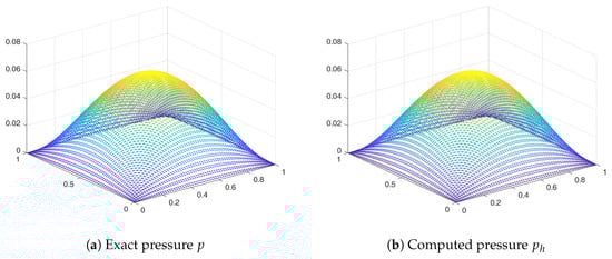
Figure 1.
Exact and computed pressure for Example 1.
Example 2.
Consider , , the source term f, and the velocity are calculated by using the exact solution:
The discrete norm errors with respect to the variable temporal steps and fixed h for two subdomains are presented in Table 5 and Table 6. The tables shows that the errors increased with time steps.
Table 5.
Discrete errors with time steps for Example 2, .
Table 6.
Discrete errors with time steps for Example 2, .
Next, the discrete errors for subdomain pressure p, the subdomain velocity , and the mortar interface pressure are presented in Table 7 and Table 8.
Table 7.
Discrete errors and convergence rates for Example 2 at time with and .
Table 8.
Discrete errors and convergence rates for Example 2 at time with and .
The discrete errors and convergence rates for Example 2 on four subdomains are represented in Table 8.
The results of our numerical experiments matched the theory established. The exact and computed solution for Example 2 are presented in Figure 2.
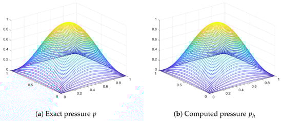
Figure 2.
Exact and computed pressure for Example 2.
It is observed from the above tables that the discrete norm errors increased with the time steps. Note that the accuracy of discrete norm error on two subdomain was better than that on four subdomains. The reason for the better accuracy on the two subdomains is stated below in the discussion of the convergence rate.
Comparing the results on two and four subdomains, we note the slightly better accuracy on the two subdomains than the four subdomains. The reason for the better accuracy on the two subdomains may be that in the case of two subdomains, we had a single interface; therefore, transmission of data across the interface was more accurate as compared to that of four subdomains. However, on two subdomains, we had large local problem, which is expensive to solve numerically. Therefore, by scarifying accuracy slightly, we have an efficient solution for the local subdomain problems.
7. Conclusions
In this article, the multiblock mortar mixed technique proposed and analyzed in [20] was extended to the second order linear parabolic problems. This approach is a combination of non-overlapping domain decomposition and the mortar finite element method. This method allowed different grids on different regions of the domain. The continuity of the flux across the subdomain interior boundary was imposed via the mortar finite element on the interface grid.
We considered the semi-discrete formulation of second order parabolic partial differential equation. The existence and uniqueness of solution for the discrete system encountered by the scheme were established. The optimal order convergence was shown for both the velocity and pressure approximations. The theoretical findings were confirmed by performing the numerical experiments for benchmark problems.
Author Contributions
The conceptualization and methodology were proposed by M.A. Software usage, problem analysis and investigation, writing of the original draft preparation, and funding acquisition by the Higher Education Commission were done by M.A. and M.S. Writing, review, and supervision were done by M.M.
Acknowledgments
This research is supported by the Higher Education Commission of Pakistan.
Conflicts of Interest
The authors declare no conflicts of interest.
References
- Brezzi, F.; Douglas, J.; Marini, L.D. Two families of mixed finite elements for second order elliptic problems. Numer. Math. 1985, 47, 217–235. [Google Scholar] [CrossRef]
- Brezzi, F.; Fortin, M.; Marini, L.D. Efficient rectangular mixed finite elements in two and three space variables. ESAIM Math. Model. Numer. Anal. 1987, 21, 581–604. [Google Scholar] [CrossRef]
- Brezzi, F.; Fortin, M. Mixed and Hybrid Finite Element Methods; Springer Series in Computational Mathematics; Springer: New York, NY, USA, 1991; Volume 15. [Google Scholar]
- Carstensen, C.; Kim, D.; Park, E.J. A priori and a posteriori pseudostress-velocity mixed finite element error analysis for the Stokes problem. SIAM J. Numer. Anal. 2011, 49, 2501–2523. [Google Scholar] [CrossRef]
- Douglas, J.; Roberts, J.E. Global estimates for mixed methods for second order elliptic equations. Math. Comput. 1985, 44, 39–52. [Google Scholar] [CrossRef]
- Duran, R. Superconvergence for rectangular mixed finite elements. Numer. Math. 1990, 58, 287–298. [Google Scholar] [CrossRef]
- Kim, D.; Park, E.J. A priori and a posteriori analysis of mixed finite element methods for nonlinear elliptic equations. SIAM J. Numer. Anal. 2010, 48, 1186–1207. [Google Scholar] [CrossRef]
- Milner, F.A. Mixed finite element methods for quasilinear second-order elliptic problems. Math. Comput. 1985, 44, 303–320. [Google Scholar] [CrossRef]
- Milner, F.A.; Park, E.J. A mixed finite element method for a strongly nonlinear second-order elliptic problem. Math. Comput. 1995, 64, 973–988. [Google Scholar] [CrossRef]
- Nédélec, J.C. Mixed finite elements in R3. Numer. Math. 1980, 35, 315–341. [Google Scholar] [CrossRef]
- Park, E.J. Mixed finite element methods for nonlinear second-order elliptic problems. SIAM J. Numer. Anal. 1995, 32, 865–885. [Google Scholar] [CrossRef]
- Raviart, P.A.; Thomas, J.M. A mixed finite element mrthod for 2nd order elliptic problems. In Mathematical Aspects of Finite Element Methods; Lecture Notes in Mathematics; Springer: New York, NY, USA, 1977; Volume 606, pp. 292–315. [Google Scholar]
- Roberts, J.E.; Thomas, J.M.; Ciarlet, P.G.; Lions, J.L. Mixed and hybrid methods. In Handbook of Numerical Analysis; North-Holland: Amsterdam, The Netherlands, 1991; Volume II, pp. 523–639. [Google Scholar]
- Arshad, M.; Park, E.J.; Shin, D.W. Analysis of multiscale mortar mixed approximation of nonlinear elliptic equations. Comput. Math. Appl. 2018, 75, 401–418. [Google Scholar] [CrossRef]
- Arbogast, T.; Estep, D.; Sheehan, B.; Tavener, S. A posteriori error estimates for mixed finite element and finite volume methods for parabolic problems coupled through a boundary. SIAM-ASA J. Uncertain. 2015, 3, 169–198. [Google Scholar] [CrossRef]
- Chen, Y.; Chen, L.; Zhang, X. Two-Grid method for nonlinear parabolic equations by expanded mixed finite element methods. Numer. Methods Part. Differ. Equ. 2013, 29, 1238–1256. [Google Scholar] [CrossRef]
- Garcia, S.M. Improved error estimates for mixed finite-element approximations for nonlinear parabolic equations: The continuous-time case. Numer. Methods Part. Differ. Equ. 1994, 10, 129–147. [Google Scholar] [CrossRef]
- Kim, M.Y.; Milner, F.A.; Park, E.J. Some observations on mixed methods for fully nonlinear parabolic problems in divergence form. Appl. Math. Lett. 1996, 9, 75–81. [Google Scholar] [CrossRef]
- Park, E.J. Mixed finite element methods for generalized Forchheimer flow in porous media. Numer. Methods Part. Differ. Equ. 2005, 21, 213–228. [Google Scholar] [CrossRef]
- Arbogast, T.; Cowsar, L.C.; Wheeler, M.F.; Yotov, I. Mixed finite element methods on non-matching multiblock grids. SIAM J. Numer. Anal. 2000, 37, 1295–1315. [Google Scholar] [CrossRef]
- Arbogast, T.; Pencheva, G.; Wheeler, M.F.; Yotov, I. A multiscale mortar mixed finite element method. Multiscale Model. Simul. 2007, 6, 319–346. [Google Scholar] [CrossRef]
- Arbogast, T.; Xiao, H. Two-level mortar domain decomposition preconditioners for heterogeneous elliptic problems. Comput. Methods Appl. Mech. Eng. 2015, 292, 221–242. [Google Scholar] [CrossRef]
- Ganis, B.; Vassilev, D.; Wang, C.; Yotov, I. A multiscale flux basis for mortar mixed discretizations of Stokes-Darcy flows. Comput. Methods Appl. Mech. Eng. 2017, 313, 259–278. [Google Scholar] [CrossRef]
- Ganis, B.; Yotov, I. Implementation of a mortar mixed finite element method using a multiscale flux basis. Comput. Methods Appl. Mech. Eng. 2009, 198, 3989–3998. [Google Scholar] [CrossRef]
- Kim, M.Y.; Park, E.J.; Thomas, S.G.; Wheeler, M.F. A multiscale mortar mixed finite element method for slightly compressible flows in porous media. J. Korean Math. Soc. 2007, 44, 1103–1119. [Google Scholar] [CrossRef]
- Peszynska, M.; Wheeler, M.F.; Yotov, I. Mortar upscaling for multiphase flow in porous media. Comput. Geosci. 2002, 6, 73–100. [Google Scholar] [CrossRef]
- Song, P.; Wang, C.; Yotov, I. Domain decomposition for stokes-darcy flows with curved interfaces. Procedia Comput. Sci. 2013, 18, 1077–1086. [Google Scholar] [CrossRef]
- Yotov, I. A multilevel Newton-Krylov interface solver for multiphysics couplings of flow in porous media. Numer. Linear Algebra Appl. 2001, 8, 551–570. [Google Scholar] [CrossRef]
- Bernardi, C.; Maday, Y.; Patera, A.T. A new nonconforming approach to domain decomposition: the mortar element method. In Nonliner Partial Differential Equations and Their Applications; Brezis, H., Lions, J.L., Eds.; Longman Scientific and Technical: London, UK, 1994. [Google Scholar]
- Ewing, R.E.; Lazarov, R.D.; Russell, T.F.; Vassilevski, P.S. Local refinement via domain decomposition techniques for mixed finite element methods with rectangular Raviart-Thomas elements. In Doamin Decomposition Methods for PDEs; Chan, T.F., Glowinski, R., Periaux, J., Widlund, O.B., Eds.; SIAM: Philadelphia, PA, USA, 1990; pp. 98–114. [Google Scholar]
- Ewing, R.E.; Wang, J. Analysis of mixed finite element methods on locally refined grids. Numer. Math. 1992, 63, 183–194. [Google Scholar] [CrossRef]
- Gaiffe, S.; Glowinski, R.; Masson, R. Domain decomposition and splitting methods for mortar mixed finite element approximations to parabolic equations. Numer. Math. 2002, 93, 53–75. [Google Scholar] [CrossRef]
- Sun, T.; Mehmani, Y.; Bhagmane, J.; Balhoff, M.T. Pore to continuum upscaling of permeability in heterogeneous porous media using mortars. Int. J. Oil Gas Coal Technol. 2012, 5, 249–266. [Google Scholar] [CrossRef]
- Wheeler, M.F.; Yotov, I. A posteriori error estimates for the mortar mixed finite element method. SIAM J. Numer. Anal. 2005, 43, 1021–1042. [Google Scholar] [CrossRef]
- Wheeler, M.F. A priori L2 error estimates for Galerkin approximations to parabolic partial differential equations. SIAM J. Numer. Anal. 1973, 10, 723–759. [Google Scholar] [CrossRef]
- Pencheva, G.; Yotov, I. Balancing domain decomposition for mortar mixed finite element methods. Numer. Linear Algebra Appl. 2003, 10, 159–180. [Google Scholar] [CrossRef]
- Yotov, I.P. Mixed Finite Element Methods for Flow in Porous Media. Ph.D. Thesis, Rice University, Houston, TX, USA, 1996. [Google Scholar]
- Grisvard, P. Elliptic Problems in Nonsmooth Domains; Pitman Advanced Pub. Program: Boston, MA, USA, 1985. [Google Scholar]
- Mathew, T.P. Domain Decomposition and Iterative Refinement Methods for Mixed Finite Element Discretisations of Elliptic Problems. Ph.D. Thesis, Courant Institute of Mathematical Sciences, New York, NY, USA, 1989. [Google Scholar]
- Ciarlet, P.G. The Finite Element Method for Elliptic Problems; Classics in Applied Mathematics Volume 40; SIAM: Philadelphia, PA, USA, 2002. [Google Scholar]
© 2019 by the authors. Licensee MDPI, Basel, Switzerland. This article is an open access article distributed under the terms and conditions of the Creative Commons Attribution (CC BY) license (http://creativecommons.org/licenses/by/4.0/).