Cooperative Co-Evolution Algorithm with an MRF-Based Decomposition Strategy for Stochastic Flexible Job Shop Scheduling

Abstract

Flexible job shop scheduling is an important issue in the integration of research area and real-world applications. The traditional flexible scheduling problem always assumes that the processing time of each operation is fixed value and given in advance. However, the stochastic factors in the real-world applications cannot be ignored, especially for the processing times. We proposed a hybrid cooperative co-evolution algorithm with a Markov random field (MRF)-based decomposition strategy (hCEA-MRF) for solving the stochastic flexible scheduling problem with the objective to minimize the expectation and variance of makespan. First, an improved cooperative co-evolution algorithm which is good at preserving of evolutionary information is adopted in hCEA-MRF. Second, a MRF-based decomposition strategy is designed for decomposing all decision variables based on the learned network structure and the parameters of MRF. Then, a self-adaptive parameter strategy is adopted to overcome the status where the parameters cannot be accurately estimated when facing the stochastic factors. Finally, numerical experiments demonstrate the effectiveness and efficiency of the proposed algorithm and show the superiority compared with the state-of-the-art from the literature.

1. Introduction

Scheduling is one of the important issues in combinational optimization problems as scheduling problems not only have theoretical significance but also have practical implications in many real-world applications [1,2]. As an extended version of job shop scheduling (JSP), flexible JSP (FJSP) considers the machine flexibility, i.e., each operation can be processed on any one machine in a given machine set. The machine flexibility makes FJSP be closer to the models in the real-world applications [3,4]. For example, the resource scheduling exists in the smart power grids system with the objective to minimize the response time with the balance of multiple resources [5,6]. In the distributed computing centers, how to allocate the limited resources to complete all tasks with the handling capacity [7]. In the logistics system or subway system, the vehicle scheduling has the same basic model of flexible scheduling in which different tasks from different users need to be transported by a set of vehicles. The objective is to transport all tasks in the minimum time with the balancing load [8], etc. All models in the mentioned real-world applications or systems are FJSP. Simply, FJSP can be denoted as the discrete optimization problem with two sub-problems, i.e., operation sequence and machine assignment, and was proved as an NP-hard problem [9].

1.1. Motivation

Various researchers concentrated on the effective algorithms for minimizing the maximum completion time which named makespan of FJSP. Lin and Gen provided a survey in 2018 and presented the information of scheduling, e.g., mathematical formulation and graph representations [10]. Chaudhry and Khan reviewed solution techniques and methods published for flexible scheduling and presented an overview of the research trend of flexible scheduling in 2016 [11]. However, most of the existing research assumes that the processing time of each operation on the corresponding machine is fixed and given in advance. In actual, the stochastic factors in the real-world applications cannot be ignored. In addition, the processing time appears to be particularly important [12]. Therefore, in this paper, we consider the stochastic FJSP (S-FJSP), and the stochastic processing time is modeled as three probability distributions, i.e., the normal distribution, the Gaussian distribution and the exponential distribution.

In recent years, various research was studied for stochastic scheduling problems. As listed in

Table 1. A summary of the fuzzy models, objectives and methodologies.

Methodologies	Distribution(s)	Objective(s) (min)
Simplified multi-objective genetic algorithm [13]	Uniform	Expected makespan
Effective multiobjective Estimation of Distribution Algorithm (EDA) [14]	Uniform	Expected makespan & total tardiness
Hybrid evolutionary algorithm [15]	Uniform	Expected makespan
Artificial bee colony algorithm [16]	Uniform; Normal; Exponent	Maximum lateness
Two-stage particle swarm optimization [17]	Uniform; Normal; Exponent	Expected total weighted tardiness
Evolutionary strategy in ordinal optimization [19]	Uniform; Normal; Exponent	Expected makespan & total tardiness
Algorithm based on artificial neural networks [18]	Uniform; Normal; Exponent	Expected makespan
Novel parallel quantum genetic algorithm [20]	Normal	Expected makespan
Cooperative coevolution genetic programming (CCGP) [21]	Uniform	Expected makespan
Co-evolutionary quantum genetic algorithm [22]	Normal	Expected makespan
Two-stage optimization [23]	Uniform; Normal; Exponent	Expected makespan

, Lei proposed a simplified multi-objective genetic algorithm (MOGA) for minimizing the expected makespan of JSP [13]. Hao et al. proposed an effective multi-objective estimation of distribution algorithm (moEDA) for minimizing the expected makespan and the total tardiness of JSP [14]. Kundakc and Kulak proposed a hybrid evolutionary algorithm for minimizing the expected of JSP makespan as well [15]. Represented by the above studies, some researchers modelled the stochastic processing timess by the uniform distribution. To show the superiority of the proposed algorithm with more conviction, various researchers modelled the stochastic processing time not only by the uniform distribution, but also by the normal distribution and the exponential distribution. Zhang and Wu proposed an artificial bee colony algorithm for minimizing the maximum lateness of JSP [16]. Zhang and Song proposed a two-stage particle swarm optimization for minimizing the expected total weighted tardiness [17]. Horng et al. and Azadeh et al. presented a two-stage optimization algorithm and an artificial neural networks (ANNs) based optimization algorithms for minimizing the expected makespan, respectively [18,19]. These studies are all ensemble algorithms with the help of the search ability of various evolutionary algorithms (EAs), e.g., genetic algorithm (GA), particle swarm optimization (PSO), etc., the local search strategies and the global search strategies. As we know, the stochastic factors result in the exponentially increasing solution space which may make EAs suffer from the performance reduction [10]. Therefore, how to increase the search ability of the proposed algorithm is quite significant for stochastic scheduling problems. Gu et al. proposed a novel parallel quantum genetic algorithm (NPQGA) for the stochastic JSP with the objective to minimize the expected makespan [20]. The NPQGA searched the optimal solution through sub-populations and some universes. As the evolutionary information exchange plays an important role in EAs as well. The parallel strategy used in NPQGA is weak in the information exchange. This weakness results in the bad cooperation with EAs for exploring and exploiting more larger solution space. Nguyen et al. presented a cooperative coevolution genetic programming for the dynamic multi-objective JSP [21]. Gu et al. studied a co-evolutionary quantum genetic algorithm for stochastic JSP [22].

Cooperative co-evolution algorithm (CEA) is widely used in the research area of a large scale optimization problem. Because the basic optimization strategy, i.e., “divide-and-conquer”, is appropriate for the problems with the increasing solution space, various researchers studied the performance of EAs applied for combinational optimization problems. However, EAs lost effectiveness as the problem scales increase, especially for FJSP [24] and the high dimensional discrete problems [25]. CEA searches the optimal solution cooperatively through decomposing the whole solution space into various sub solution spaces. Therefore, the decomposition strategy is significant because the performance of CEA is sensitive to the decomposition status [26]. Various researchers studied the decomposition strategies [27,28,29]. However, they mainly focus on the optimization of mathematical function problems. The existing decomposition strategies cannot be used for combinational optimization problems directly because of the precedence constraint and dependency relationship among the decision variables.

The existing decomposition strategies can be divided into two categories, the non-automatic decomposition and the automatic decomposition. The non-automatic decomposition strategy contains three types, i.e., one-dimension decomposition strategy, random decomposition strategy and extended decomposition strategy. They all decompose the decision variables according to the random technique with no consideration of correlation among the decision variables. The automatic decomposition strategies consider and detect the correlation among decision variables through various techniques, i.e., delta grouping, K-means clustering algorithm, cooperative co-evolution with variable interaction learning (CCVIL), interdependence learning (IL), fast interdependency identification (FII), differential grouping (DG), the extended differential grouping (EDG), etc. The detail decomposition methodologies, advantages and disadvantages are listed in

Table 2. A summary of the definition, advantages and disadvantages of the existing decomposition strategies.

Strategy	Methodologies	Advantage(s)	Disadvantage(s)
One-dimension [31]	Decompose N variables into N groups	Easy to implement with low cost	Lose efficacy on non-separable problems
Random [32]	Randomly decompose N variables into k groups	Dependency on random technique	Lose efficacy on non-separable problems
Set-based [33]	Random decompose N variables based on set	Effective than one-dimension strategy	Lose efficacy on non-separable problems
Delta [28]	Detect relationship based on the averaged difference	More effective than random grouping	Lose efficacy on non-separable problems
K-means [34]	Detect relationship based on K-means algorithm	Effective on unbalanced grouping status	High computational cost
CCVIL [35]	Detect relationship based on non-monotonicity method	Effective than manual strategies	Exist insurmountable benchmark
IL [36]	Detect relationship only once for each variable	Lower computational cost than CCVIL	Worse performance than CCVIL
FII [37]	Detect through fast interdependency identification	Lower computational cost than CCVIL	Worse performance for conditional variable
DG [38]	Detect relationship by the variance of fitness	Better performance combined with PSO	High computational cost
EDG [39]	Detect relationship by the variance of fitness	Better performance compared with PSO	High computational cost

. Therefore, the detection methodologies for the correlation among the decision variables has a strong effect on the performance of CEA [30]. However, the performance of the automatic decomposition strategy is better than the non-automatic decomposition strategy, the high computational cost is always high, which is taboo for combinational optimization problems, especially for FJSP due to the complex decoding process.

Probabilistic graphical models (PGMs) consist of Bayesian networks (BNs) and Markov random fields (MRFs). BNs are directed acyclic graphs which used for representing the causal relationship. MRFs are undirected graphs which are used for representing the dependency relationship. BNs and MRFs can provide the intuitive representation of joint probability distributions of the decision variables. Various researchers learned the correlation among decision variables with taking the problem characteristics and the graph characteristics into consideration according to the network structure of MRFs [40,41]. Moreover, MRFs are widely used in many research areas in recent years. Sun et al. proposed a supervised approached to detect the relationship of variables to implement image classification according to the weighted MRFs [42]. Li and Wand studied a combination of convolutional neural networks and MRFs to implement image synthesis [43], etc. Paragios and Ramesh studied a variable detection approach with the minimization techniques that are based on the learned MRF structure for solving the subway monitoring problem in the real-time environment [44]. Tombari and Stefano presented an automatic 3D segment algorithm according to the learned variable relationship by the structure of MRF [45]. Various researchers have been denoted to detect the relationship for decomposing decision variables.

1.2. Contribution

In this paper, a decomposition strategy considering a Markov random field which is called an MRF-based decomposition strategy is proposed. All decision variables are decomposed according to the network structure of MRF with respect to the estimated parameters. The decision variables are decomposed into two sets, and the redefined correlation between two variables is used for detecting the correlation relationship. The hybrid cooperative co-evolution with the MRF-based decomposition strategy is called hCEA-MRF. The hCEA-MRF decomposes the whole solution space into various sub small solution spaces and searches the optimal solution cooperatively. This increases the probability of searching out the optimal solution for the stochastic problems.

• A cooperative co-evolution framework is improved and adopted. In the improved framework, CEA works iteratively within each sub solution space until the termination criterion matches. All sub solution spaces are evoluted cooperatively, and the suitable representation selection strategy helps hCEA-MRF find the optimal solution.
• An MRF-based decomposition strategy is proposed for decomposing the decision variables into various decompositions. All decision variables are decomposed according to the network structure with respect to the estimated parameters. The decision variables which are put into the same decomposition are viewed as the strong relevance among each other. Each decomposition is associated with a sub solution space.
• A self-adaptive parameter mechanism is designed. Instead of the general linearity and nonlinearity self-adaptive mechanism, our proposed self-adaptive mechanism is based on the performance, i.e., the number and the percentage of the individuals generated by the current parameters successfully and unsuccessfully go into the next generation.

The rest of the paper is organized as follows: Section 2 introduces the formulation model of flexible scheduling. Section 3 describes the proposed hCEA-MRF in detail. The numerical experiments are designed and analyzed in Section 4 and Section 5 presents the conclusions.

2. Formulation Model of S-FJSP

As an extended version of the standard JSP, FJSP gives the wider availability of machines for each operation. JSP obtains the minimum makespan by finding the optimal operation sequence while FJSP needs to assign the suitable machines to each ordered operation one at a time. The makespan is defined as the maximum completion time of all jobs. There exist some assumptions for FJSP. There are strict precedence constraints among the operations of the same jobs but no precedence constraints of different jobs. Each machine is available from time zero and only can process one operation without any interruption at a time. Each operation can only be processed once as well. The setup times among different machines are involved in the processing times, and all processing times are fixed and given in advance. The main difference between S-FJSP and FJSP is that the processing times of the operations in S-FJSP are not fixed and cannot be known in advance until the schedule is completed. In this paper, a pure integer programming model is adopted to model S-FJSP with transmuting the stochastic processing times. The processing time ($\xi p_{ikj}$) of each operation ($O_{ij}$) on $M_j$ belongs to a probability with the given distribution parameters, i.e., the expected value ($E\left[\xi p_{ikj}\right]$) and the variance value ($V_{ij}$). In this paper, three probability distributions, i.e., the uniform distribution, the Gaussian distribution, and the exponential distribution, are used for predicting $\xi p_{ikj}$. Consequently, the concept scenario $\xi$ is used for constructing the uncertainty. The notations used in this paper are listed as follows:

Indices:

$$\begin{array}{cc}\hfill i& \mathrm{the}\mathrm{index}\mathrm{of}\mathrm{job}(i=1,2,\dots ,n),\hfill \\ \hfill j& \mathrm{the}\mathrm{index}\mathrm{of}\mathrm{machine}(j=1,2,\dots ,m),\hfill \\ \hfill k& \mathrm{the}\mathrm{index}\mathrm{of}\mathrm{operation}(k=1,2,\dots ,n_i),\hfill \end{array}$$

Parameters:

$$\begin{array}{cc}\hfill n& \mathrm{the}\mathrm{total}\mathrm{number}\mathrm{of}\mathrm{jobs},\hfill \\ \hfill m& \mathrm{the}\mathrm{total}\mathrm{number}\mathrm{of}\mathrm{machines},\hfill \\ \hfill n_i& \mathrm{the}\mathrm{total}\mathrm{number}\mathrm{of}\mathrm{operations}\mathrm{belonging}\mathrm{to}\mathrm{job}{J}_i,\hfill \\ \hfill O_{ik}& \mathrm{the}k\mathrm{th}\mathrm{operation}\mathrm{of}\mathrm{job}{J}_i,\hfill \\ \hfill M_{ik}& \mathrm{the}\mathrm{assigned}\mathrm{machine}\mathrm{index}\mathrm{of}{O}_{ik},\hfill \\ \hfill \xi p_{ikj}& \mathrm{the}\mathrm{processing}\mathrm{time}\mathrm{of}{O}_{ik}\mathrm{on}{M}_j,\hfill \end{array}$$

Decision variables:

$$\begin{array}{cc}\hfill x_{ikj}& 0\mathrm{or}1,\mathrm{opeartion}{O}_{ik}\mathrm{assigned}\mathrm{on}\mathrm{machine}{M}_j,\hfill \\ \hfill \xi t_{ikj}^S& \ge 0,\mathrm{the}\mathrm{start}\mathrm{time}\mathrm{of}\mathrm{operation}{O}_{ik}\mathrm{on}{M}_j,\hfill \\ \hfill \xi t_{ikj}^T& \ge 0,\mathrm{the}\mathrm{end}\mathrm{time}\mathrm{of}\mathrm{operation}{O}_{ik}\mathrm{on}{M}_j.\hfill \end{array}$$

The objective function of S-FJSP is to minimize the expected makespan:

$$\begin{array}{cc}min& E[C_{\max }]=E[\underset{i}{max}\{\underset{k}{max}\{\underset{j}{max}\xi t_{ikj}^T\}\}],\hfill \end{array}$$

(1)

where $\xi t_{ikj}^T=\xi t_{ikj}^S+\xi p_{ikj}$. During the process of the whole scheduling, each operation is only processed on one machine. In other words, all decision variables $x_{ikj}$ need to summed as 1.

$$\begin{array}{c}\hfill \sum _{j=1}^m{x}_{ikj}\le 1,\forall i,k.\end{array}$$

(2)

As discussed, there exist the precedence constraint of the operations within each job, i.e., the successor operation needs to begin after the completion of the preorder operation. Thus, the start time of the successor operation needs to be larger than the end time of the preorder operation:

$$\begin{array}{c}\hfill \xi t_{ikj}^S-\xi t_{i{k}^{\prime }j}^T\ge 0,\forall i,(k\succ k^{\prime }).\end{array}$$

(3)

Each operation cannot be interrupted, i.e., the successor operation on the same machine can only begin when the preorder operation on the same machine finishes and the preorder operation in the same job finishes:

$$\begin{array}{c}\hfill (\sum _{i=1}^n\sum _{k=1}^{n_i}{x}_{ikj}·\xi t_{ikj}^S\le \sum _{i=1}^n\sum _{k^{\prime }=1}^{n_i}{x}_{i{k}^{\prime }j}·\xi t_{i{k}^{\prime }j}^S)\wedge (\sum _{i=1}^n\sum _{k=1}^{n_i}{x}_{ikj}·\xi t_{ikj}^T\le \sum _{i=1}^n\sum _{k^{\prime }=1}^{n_i}{x}_{i{k}^{\prime }j}·\xi t_{i{k}^{\prime }j}^S),\forall j.\end{array}$$

(4)

Finally, some non-negative value restrictions of the decision variables are needed. The decision variable $x_{ikj}$ can only be 0 or 1. When $x_{ikj}$ is equal to 1, it means $O_{ik}$ is assigned on machine $M_j$; otherwise, it means $O_{ik}$ is not assigned on machine $M_j$. The start time and the end time of any operation need to be larger than 0:

$$\begin{array}{c}\hfill x_{ikj}\in \{0,1\},\forall i,j,k,\end{array}$$

(5)

$$\begin{array}{c}\hfill t_{ikj}^S,t_{ikj}^T\ge 0,\forall i,k,j.\end{array}$$

(6)

3. The Implement of hCEA-MRF

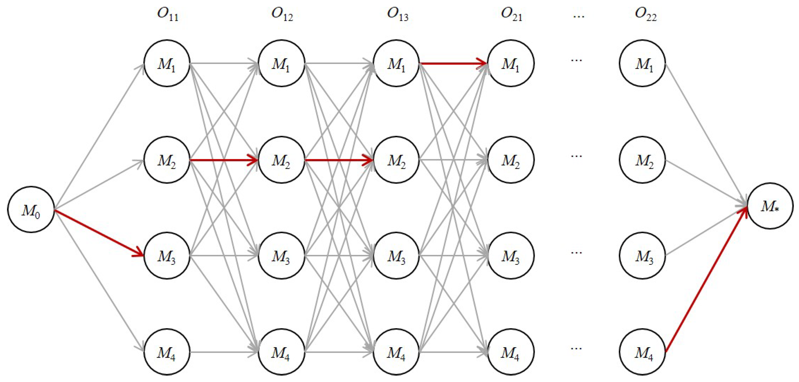
In this section, the hybrid cooperative coevolution algorithm with MRF-based decomposition strategy (hCEA-MRF) is proposed for solving the flexible scheduling with the stochastic processing times for minimizing the expected makespan. The hCEA-MRF is described as follows: First, a real number representation for PSO is adopted. The fractional part and the integral part represent the priority of operation sequence and machine assignment, respectively. Then, the CEA is improved for maintaining more optimized information for each cooperative sub solution space. Considering the correlation relationship, the MRF-based decomposition strategy groups all decision variables according to the learned network structure of MRF. Finally, two points’ critical path-based local search strategy is used for enhancing the search ability of hCEA-MRF. All details are introduced as follows, and the pseudocode is summarized in Algorithm 1.

3.1. Representation

The design of the representation of the candidate solutions plays an important role in the research of EAs. Designing an effective representation contains the following aspects [10]:

• The genotype space needs to cover as many as possible candidate solutions in order to search out the optiml solution.
• The necessary decode time needs to be as short as possible.
• Each representation needs to be corresponding to a feasible candidate solution, and the new representation which has completed evolutionary operators needs to be corresponding to a feasible candidate solution as well.

In this paper, we adopt the random-key based representation. It encodes one candidate solution with some random generated real numbers. Each real number ($x_{ij}\left(\phi \right)$) consists of two parts, i.e., an integral part and a fractional part. The integral part and the fractional part are randomly generated from $[1,m]$ and $[0,1]$, respectively. An illustration of a random-key based representation for a simple example with full complexity (shown in

Table 3. An instance of flexible job shop scheduling.

Job	Operation	${\mathit{M}}_1$	${\mathit{M}}_2$	${\mathit{M}}_3$	${\mathit{M}}_4$
$J_1$	$O_{11}$	2	3	3	3
	$O_{12}$	4	1	3	2
	$O_{13}$	3	2	3	4
$J_2$	$O_{21}$	3	3	2	1
	$O_{22}$	3	2	2	4
	$O_{23}$	3	2	3	2
$J_3$	$O_{31}$	3	2	3	2
	$O_{32}$	2	2	3	4

) is given in Figure 1. The sorted fractional part of each operation is used for decoding the representation of a candidate problem solution and provides the priority set of operations: {0.21, 0.16, 0.77, 0.15, 0.42, 0.09, 0.18, 0.66}. Considering the priority-based decoding process, sorting the fractional part provides the operations sequence (OS): $\{O_{11},O_{31},O_{32},O_{12},O_{13},O_{21},O_{22},O_{23}\}$. The integral part is in charge of the machine assignment (MA) for the corresponding operation and provides MA: $\{M_3,M_2,M_2,M_1,M_3,M_3,M_2,M_4\}$. The illustration of machine assignment is shown in Figure 2. The makespan is 10, and the Gantt chart is shown in Figure 3. The reason why we adopt random-key based representation is that the random-key based representation can represent a larger solution space and each decoded solution is ensured as a feasible solution. These two points guarantee the searching efficiency and the probability of searching out an optimal solution.

Algorithm 1 The procedure of hCEA-MRF.

Require: problem data, problem model, parameters

Ensure:$g_{best}$;

1:  Initialize the population randomly; 2:  while ($\tau <T$) do 3:      if $\tau =1$ or Regrouping is true then 4:          Sampling the individuals; 5:          Pre-process to obtain the best individuals and the corresponding critical paths; 6:          MRF network structure learning; 7:          MRF network parameters estimating; 8:         Decompose sub-components according to the learned structure and estimated parameters; 9:      end if 10:     for each sub-component s do 11:         $\phi \leftarrow 0$ 12:         while ($\phi <t$) do 13:            for each $sub\_ind\left(\phi \right)$ do 14:                if $\mathit{e}$ ($\mathit{r}$(s,$sub\_ind\left(\phi \right)$,$p_{best}\left(\phi \right)$))< $\mathit{e}$ ($p_{best}\left(\phi \right)$) then 15:                    $\mathit{r}$(s,$p_{best}\left(\phi \right)$,$sub\_ind\left(\phi \right)$); 16:                end if 17:                if $\mathit{e}$ ($\mathit{r}$(s,$p_{best}\left(\phi \right)$,$s{g}_{best}\left(\phi \right)$))< $\mathit{e}$ ($s{g}_{best}\left(\phi \right)$) then 18:                    $\mathit{r}$(s,$s{g}_{best}\left(\phi \right)$,$pbest\left(\phi \right)$); 19:                end if 20:            end for 21:            $\phi \leftarrow \phi +1$ 22:         end while 23:         for each $sub\_ind\left(\phi \right)$ do 24:            ${\mathit{up}}_{\mathit{l}}$($l_{best}\left(\phi \right)$); 25:         end for 26:         if $\mathit{e}$ ($\mathit{r}$(g,$s{g}_{best}\left(\phi \right)$,$g_{best}$))< $\mathit{e}$ ($g_{best}\left(\phi \right)$) then 27:              $\mathit{r}$(g,$g_{best}$,$s{g}_{best}\left(\phi \right)$); 28:         end if 29:         Self-adaptive parameters strategy; 30:     end for 31: end while 32: return$g_{best}$;

3.2. CEA

3.2.1. Evolutionary Strategy

The initialization of the individuals of PSO decides the initial search point while the update strategy decides the future detection direction and the length of moving steps. The traditional update strategy considers the global best solution ($g_{best}\left(\phi \right)$) and the personal best solution ($p_{best}\left(\phi \right)$). Thus, PSO with the traditional update strategy has good global search ability but no good ability of neighborhood search as both kinds of history best solutions can only give global guidance [11]. Moreover, EAs always need the cooperation of exploration and exploitation, especially for the stochastic environment. Therefore, we adopt two update strategies with the cooperation of two distributions for the individuals of PSO. Two distributions are the normal distribution and the Cauchy distribution, respectively. The normal distribution is used for sampling new individuals among the neighbourhood structure while the Cauchy distribution is used for exploiting solution spaces more widely. The new written update strategy is:

$$x_{ij}(\phi +1)=\left\{\begin{array}{c}{p}_{best}\left(\phi \right)+\mathcal{C}\left(1\right)·|p_{best}\left(\phi \right)-l_{best}\left(\phi \right)|,\mathrm{if}rand(0,1)\ge p,\hfill \\ l_{best}\left(\phi \right)+\mathcal{N}(0,1)·|p_{best}\left(\phi \right)-l_{best}\left(\phi \right)|,\mathrm{otherwise},\hfill \end{array}\right.$$

(7)

where $\mathcal{N}(0,1)$ and $\mathcal{C}\left(1\right)$ represent the numbers randomly generated by a normal distribution with parameters 0 and 1 and a Cauchy distribution with parameter 1. For each iteration, a random number is generated. If the random number is larger than the given p, $x_{ij}(\phi +1)$ is updated according to equation with Cauchy distribution. Otherwise, $x_{ij}(\phi +1)$ is updated according to equation with normal distribution. $l_{best}\left(\phi \right)$ stands for the best local individual in the $\phi$th generation. It is defined as the best individual among three adjacent individuals in the population, and it is updated at the end of each iteration. A critical path-based local search is used in our hCEA-MRF for searching for better solutions and increasing the local search ability.

3.2.2. CEA Evaluation

CEA is an evolutionary computation approach which works through the core idea of “divide and conquer” to divide one large scale solution space into various subcomponents, and all divided components are evaluated cooperatively through multiple optimizers until the maximum generations (T) is reached. As described in Algorithm 1, $\mathit{e}$() is a function which is used for evaluating the makespan, and $\mathit{r}(s,target,trail)$ returns a new individual which is the copy of $target$ with the sth component replaced by the sth component of $trail$. If $\mathit{e}$($\mathit{r}(s,su{b}_{ind}\left(\phi \right),p_{best}\left(\phi \right)$) is better than $\mathit{e}$($p_{best}\left(\phi \right)$). It illustrates that the sth sub-component of $su{b}_{ind}\left(\phi \right)$ has positive effects on improving $p_{best}\left(\phi \right)$. Then, the sth sub-component of $p_{best}\left(\phi \right)$ is replaced with s th sub-component of $su{b}_{ind}\left(\phi \right)$ (line: 13–15). $s{g}_{best}\left(\phi \right)$ (line: 16–18) and $g_{best}$ (line: 25–27) are updated in the same manner. CEA works for each sub-component for t generations in order to maintain the best historical information and search the optimal solution. ${\mathit{up}}_{\mathit{l}}$ works through updating the best local individual with the best personal individual among three adjacent individuals in the whole population.

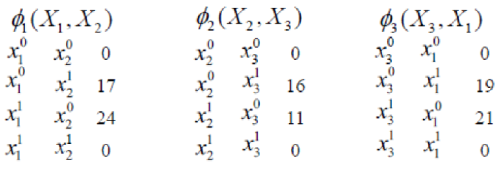
3.3. MRF-Based Decomposition Strategy

MRF (G, $\mathrm{\Phi }$) is an undirected graph which can represent the correlation relationship among the decision variables. The network structure ($G=(\mathrm{\Omega },A)$) consists of a set of nodes ($\mathrm{\Omega }$) and a set of undirected arcs (A). Two nodes linked with one undirected arc means that they have the correlation relationship. $\mathrm{\Phi }$ represents the parameters of MRF. The network structure used in our MRF-based decomposition strategy consists of D nodes where D is equal to the length of the individual, i.e., the total number of all operations. We use each node ($x_h$ simply for $x_{ij}$) to represent each gene (random key) in the individual, i.e., each node is corresponding to each operation.

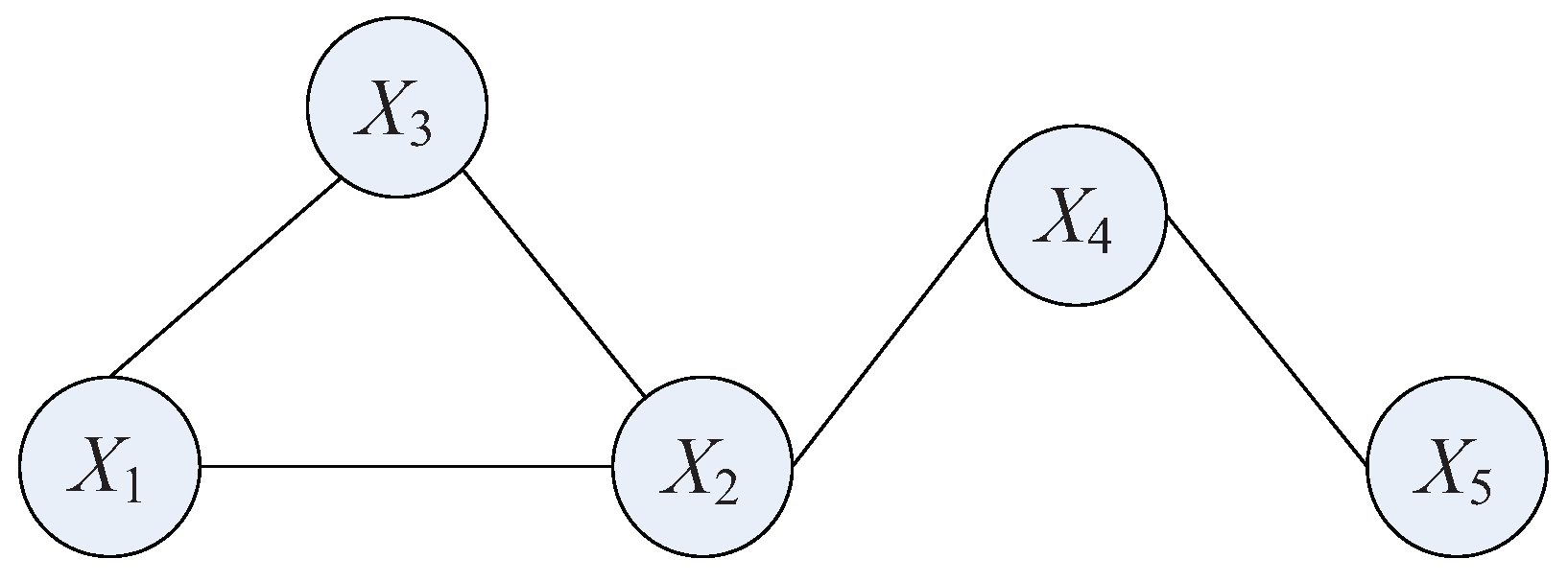
3.3.1. MRF Structure Learning

During the period of preprocessing, various individuals are sampled and evaluated according to the classical PSO update strategy for $\pi$ generations. $\pi$ best global individuals are recorded and restored. Each individual contains one critical path. Thus, at least $\pi$ critical pathes are obtained. Then, the probability ($P_{cp}$) of each operation (node) belonging to the critical operation (node) can be estimated as well. As the critical path is a key factor for scheduling problems, only the change of the length of the critical path has a chance to change the final makespan. Therefore, we divide all nodes into two sets, i.e., the set of parent nodes (${\mathrm{\Omega }}_{prt}$) and child nodes (${\mathrm{\Omega }}_{cld}$). The nodes with higher $P_{cp}$ are put into the set of parent nodes while the rest of the nodes are put into the set of children nodes.

The correlation among the variables is important for learning the network structure. To illustrate clearly, we use ${\omega }_{prt}$ and ${\omega }_k$ to represent the nodes in ${\mathrm{\Omega }}_{prt}$ and ${\mathrm{\Omega }}_k$, respectively. We use $V({\omega }_k/{\omega }_{prt})$ to represent the difference value which is the value before and after deleting ${\omega }_{prt}$ in the critical path. $V({\omega }_k/{\omega }_{prt})$ is defined and calculated in Equation (8). The large $V({\omega }_k/{\omega }_{prt})$ stands for the strong correlation between ${\omega }_{prt}$ and ${\omega }_k$; otherwise, the small $V({\omega }_k/{\omega }_{prt})$ stands for the weak correlation between ${\omega }_{prt}$ and ${\omega }_k$:

$$\begin{array}{c}\hfill V({\omega }_k/{\omega }_{prt})=\frac{1}{\mathcal{Z}}\sum _{k=1}^{\pi }(L_S({\omega }_k/{\omega }_{prt})-E_S({\omega }_k/{\omega }_{prt})),\end{array}$$

(8)

where $\pi$ is the number of obtained solutions in the preprocessing, and $\mathcal{Z}$ is the normalization function. $E_S({\omega }_k/{\omega }_{prt})$ and $L_S({\omega }_k/{\omega }_{prt})$ return the earliest starting time and the latest starting time of ${\omega }_k$ after deleting the critical node ${\omega }_{prt}$, respectively. Each ${\omega }_k$ will be linked with ${\omega }_{prt}$ with the highest value of V because the higher value, the stronger correlation do ${\omega }_k$ and ${\omega }_{prt}$ have. The network structure can be constructed through traversing all children nodes. We assume $\left|\mathrm{\Omega }\right|=a$, $|{\mathrm{\Omega }}_{prt}|=b$; then, $|{\mathrm{\Omega }}_{cld}|=a-b$. Constructing the network structure has $b\times (a-b)$ computational complexity, i.e., $\mathcal{O}\left(n\right)$.

3.3.2. MRF Parameters Learning

There exists one set of potential functions which is called “factor” for MRF, and it is a nonnegative real function defined on the subset of variables to define the probability distribution functions. For any subset of nodes in G, if there exists the connection in any pair of nodes, the subset of nodes is called “clique”. If any one node cannot be added into the clique to form a new clique, this clique is called “maximal clique”, i.e., the maximal clique is the one which cannot be included by other cliques. As shown in Figure 4, $\{X_1,X_2,X_3\}$, $\{X_3,X_4\}$, $\{X_4,X_5\}$ are the maximal cliques. Obviously, each node appears in at least one clique.

In MRF, the joint probability distribution (JPD) can be used for estimating the relationship between two linked variables. It be calculated by the product of multiple factors based on the decomposition cliques. To illustrate clearly, we use $Q\in \mathcal{C}$ to represent a set of cliques is $Q\in \mathcal{C}$, and $x_Q$ represents the variable set corresponding to Q. The JPD can be calculated as:

$$\begin{array}{c}\hfill P\left(Y\right)=\frac{1}{\mathcal{W}}\prod _{Q\in \mathcal{C}}{\psi }_Q\left(x_Q\right),\end{array}$$

(9)

where ${\psi }_Q$ is the potential function corresponding to Q for modeling the variables within Q, and $\mathcal{W}$ is a normalizing factor for ensuring the correction of $P\left(X\right)$. The JPD of X in Figure 4 can be calculated as:

$$\begin{array}{c}\hfill P\left(Y\right)=\frac{1}{\mathcal{W}}{\psi }_{123}(X1,X_2,X_3){\psi }_{34}(X_3,X_4),{\psi }_{45}(X_4,X_5).\end{array}$$

(10)

The factors of $X_1$, $X_2$ and $X_3$ are shown in Figure 5. $x_1^0$ and $x_1^1$ represent that $X_1$ is a critical node or non-critical node, respectively. The number in Figure 5 represents the solution numbers that conform to the combination of $x_1^0$ and $x_1^1$. For example, 17 means that there exist 17 solutions in which $X_1$ is a non-critical node while $X_2$ is a critical node. We model the variables within the factors, and the JPD of $X_1$, $X_2$ and $X_3$ is rewritten as follows:

$$\begin{array}{c}\hfill P(X_1,X_2,X_3)=\frac{1}{\mathcal{W}}{\psi }_{12}(X_1,X_2)·{\psi }_{23}(X_2,X_3)·{\psi }_{31}(X_3,X_1),\end{array}$$

(11)

where

$$\begin{array}{c}\hfill \mathcal{W}={\mathrm{\Sigma }}_{X_1,X_2,X_3}{\psi }_{12}(X_1,X_2)·{\psi }_{23}(X_2,X_3)·{\psi }_{31}(Y_3,Y_1).\end{array}$$

(12)

In order to obtain the marginal probability (MP) of $X_2$, we can sum out the JPD of $X_1$ and $X_3$. The MP and the network structure are collaborated to decompose the nodes. Each parent node leads a simple group, and the child nodes are grouped based on the MP. Each child node is grouped with the parent node with the highest MP. In this way, all nodes (variables) can be decomposed into several groups.

3.4. Parameters Self-Adaptive Strategy

Parameters of EAs play an important role, and various researchers studied how to find or set the suitable parameters for decades [10]. However, the fixed parameters cannot meet all statuses when facing the stochastic factors. Thus, our hCEA-MRF only gives an initial value of the selection probability ($p=0.5$) of update equations, and p is updated for each 15 iterations. The exact value is self-adjusted in the process of optimization according to the performance of the population. The self-adaptive strategy is listed in:

$$\begin{array}{c}\hfill p=\left\{\begin{array}{c}\mathbf{N}(0.5,0.3),\mathrm{if}\mathbf{U}(0,1)<\varpi ,\hfill \\ \xi ,\mathrm{otherwise},\hfill \end{array}\right.\end{array}$$

(13)

where $\omega$ stands for the selection probability of update equations for p, and the initial value of $\omega$ is 0.5. $\omega$ is updated for each 50 iterations. Obviously, self-adaptive $\omega$ is more suitable than a fixed value as well. Thus, our hCEA-MRF adopts the Equation (14) for self-adapting $\omega$:

$$\begin{array}{c}\hfill \varpi =\frac{{\theta }_1({\theta }_2+{\lambda }_2)}{{\theta }_2({\theta }_1+{\lambda }_1)+{\theta }_1({\theta }_2+{\vartheta }_2)},\end{array}$$

(14)

where ${\theta }_1$ and ${\theta }_2$ account for the numbers of individuals that are selected into the next generation updated by the update equation with the Cauchy distribution and the normal distribution, respectively. ${\lambda }_1$ and ${\lambda }_2$ account for the numbers of individuals that are abandoned to next generational evaluation by the update equation with the Cauchy distribution and the normal distribution, respectively.

4. Simulation Experiments

In this section, the description of the simulation experiments and the discussion of experiments results are introduced and analyzed. To guarantee the fairness, our proposed algorithm and all compared algorithms are implemented in the same hardware environment, i.e., a computer with Inter (R) Core(TM) i7-4790 CPU (Dell Inc., Round Rock, TX, USA) @3.60GHZ with 12 GB RAM. To evaluate the effectiveness of our proposed algorithm under the stochastic environment, each experiment runs 30 independent repeats. Three state-of-the-art, i.e., hybrid GA (HA) [46], hybrid PSO (HPSO) [47], hybrid harmony search and large neighborhood search (HHS/LNS) [48] are tested and compared. The used parameters, i.e., T, t, $\pi$ are set to 20, 10, 100, respectively.

4.1. Description of the Dataset

As discussed above, the stochastic factors among the processing times in real world applications cannot be ignored. Thus, we model the stochastic processing times with three distributions, i.e., the uniform distribution, the Gaussian distribution and the exponential distribution. We choose the widely tested benchmark BRdata which was first proposed by Brandimarte as the basic benchmark. BRdata consists of 10 instances whose scale varies from 10 jobs and six machines to 20 jobs and 15 machines. For the uniform distribution, the parameter $\delta$ is set to be 0.2 which means that the stochastic processing times are randomly generated from $[(1-\delta )p_{ijk},(1-\delta )p_{ijk}]$, where $p_{ikj}$ represents the determined processing time. For the Gaussian distribution, the stochastic processing times are randomly generated from Gaussian distribution with two parameters, $\alpha$ and $\beta$, where $\alpha$ and $\beta$ are set to $p_{ikj}$ and round($0.5\ast p_{ikj}$). round stands for the function that returns a rounded integer value. For the exponential distribution, the parameters are set to $p_{ikj}$ and $\frac{1}{p_{ikj}}$. All parameter settings are referred to [19]. The new generated benchmarks are named according to different probability distributions. For example, for the classical instances in BRData, i.e., Mk01 [49], the generated instances with the uniform distribution, the Gaussian distribution and the exponential distribution are named as UMk01, GMk01 and EMk01, respectively.

4.2. Superiority of hCEA-MRF

4.2.1. Performance Compared with State-of-the-Art

To verify the effectiveness, we compare our hCEA-MRF with three state-of-the-art ones on the generated instances with three distributions. The average (Average) and standard variance (Variance) as shown in

Table 4. The performance compared with the state-of-the-art for the generated instances by uniform distribution.

	HA		HPSO		HHS/LNS		hCEA-MRF
	Average	Variance	Average	Variance	Average	Variance	Average	Variance
UMk01	40.6	2.3	40.8	2.5	40.2	1.5	39.8	1.9
UMk02	27.1	2.4	27.3	2.1	26.5	1.7	25.9	1.4
UMk03	206.7	43.1	206.5	42.7	206.6	42.8	205.2	41.1
UMk04	62.1	2.3	61.7	2.1	62.1	2.3	60.8	1.7
UMk05	173.4	5.7	174.1	5.3	172.3	5.5	171.1	4.6
UMk06	60.6	4.6	61.4	4.8	60.6	4.3	58.6	3.7
UMk07	142.5	13.1	141.6	12.8	140.4	12.1	138.4	11.8
UMk08	525.3	102.7	524.6	103.2	523.4	102.1	522.3	101.7
UMk09	304.3	161.2	303.8	161.4	304.2	160.3	302.3	156.9
UMk10	203.1	4.4	202.7	5.3	201.3	5.7	198.8	4.6

,

Table 5. The performance compared with the state-of-the-art for the generated instances by Gaussian distribution.

	HA		HPSO		HHS/LNS		hCEA-MRF
	Average	Variance	Average	Variance	Average	Variance	Average	Variance
GMk01	41.6	2.6	42.1	2.9	41.3	2.0	40.7	2.3
GMk02	27.5	2.4	26.7	2.4	26.9	2.1	26.3	1.9
GMk03	207.9	46.5	208.4	47.2	206.7	45.5	206.4	44.7
GMk04	63.2	3.6	63.6	3.1	62.9	2.6	61.6	2.3
GMk05	175.4	6.5	176.2	5.8	174.5	6.2	173.2	5.5
GMk06	62.3	5.7	61.5	4.9	60.4	4.2	60.1	4.5
GMk07	144.5	14.2	142.7	13.8	142.9	13.1	141.4	12.9
GMk08	532.1	106.5	527.4	105.5	525.3	103.8	524.6	104.8
GMk09	305.4	167.2	307.2	164.3	305.5	163.3	303.5	162.4
GMk10	205.6	6.1	205.6	9.5	204.6	7.9	202.8	6.8

and

Table 6. The performance compared with state-of-the-art for the generated instances by exponential distribution.

	HA		HPSO		HHS/LNS		hCEA-MRF
	Average	Variance	Average	Variance	Average	Variance	Average	Variance
EMk01	44.5	4.7	43.8	4.3	42.8	2.5	42.3	3.1
EMk02	29.4	3.3	28.7	3.6	28.1	2.8	27.2	2.5
EMk03	209.4	45.3	208.4	44.6	208.1	43.8	207.2	43.2
EMk04	64.2	3.1	63.8	3.4	63.1	2.5	62.1	2.7
EMk05	174.5	7.8	175.4	7.1	174.2	6.6	173.2	6.5
EMk06	142.3	14.6	141.8	13.8	141.2	13.5	140.2	13.2
EMk07	526.4	104.6	527.1	105.5	525.3	101.3	524.5	103.2
EMk08	306.3	160.4	304.6	159.3	304.6	158.6	303.5	158.4
EMk09	207.4	6.4	206.5	6.7	206.1	6.1	205.8	5.9
EMk10	207.2	5.6	207.3	6.0	207.2	7.9	205.8	5.9

are used for evaluating the performance. The bold numbers represent the best performance in each line, and they have the same meanings in the whole paper. We can see that our hCEA-MRF can get the minimum average and variance of makespan in 30 scenarios for all instances with three probability distributions. The reasons for this can be analyzed as follows:

• The improved cooperative coevolution with the help of the new written update strategy of PSO searches the optimal solution in multiple sub solution spaces.
• The MRF-based decomposition strategy considers the relationship among variables instead of decomposing them only based on the random technique.
• The parameter self-adaptive strategy works in the process of optimization instead of the fixed parameters when facing stochastic factors.

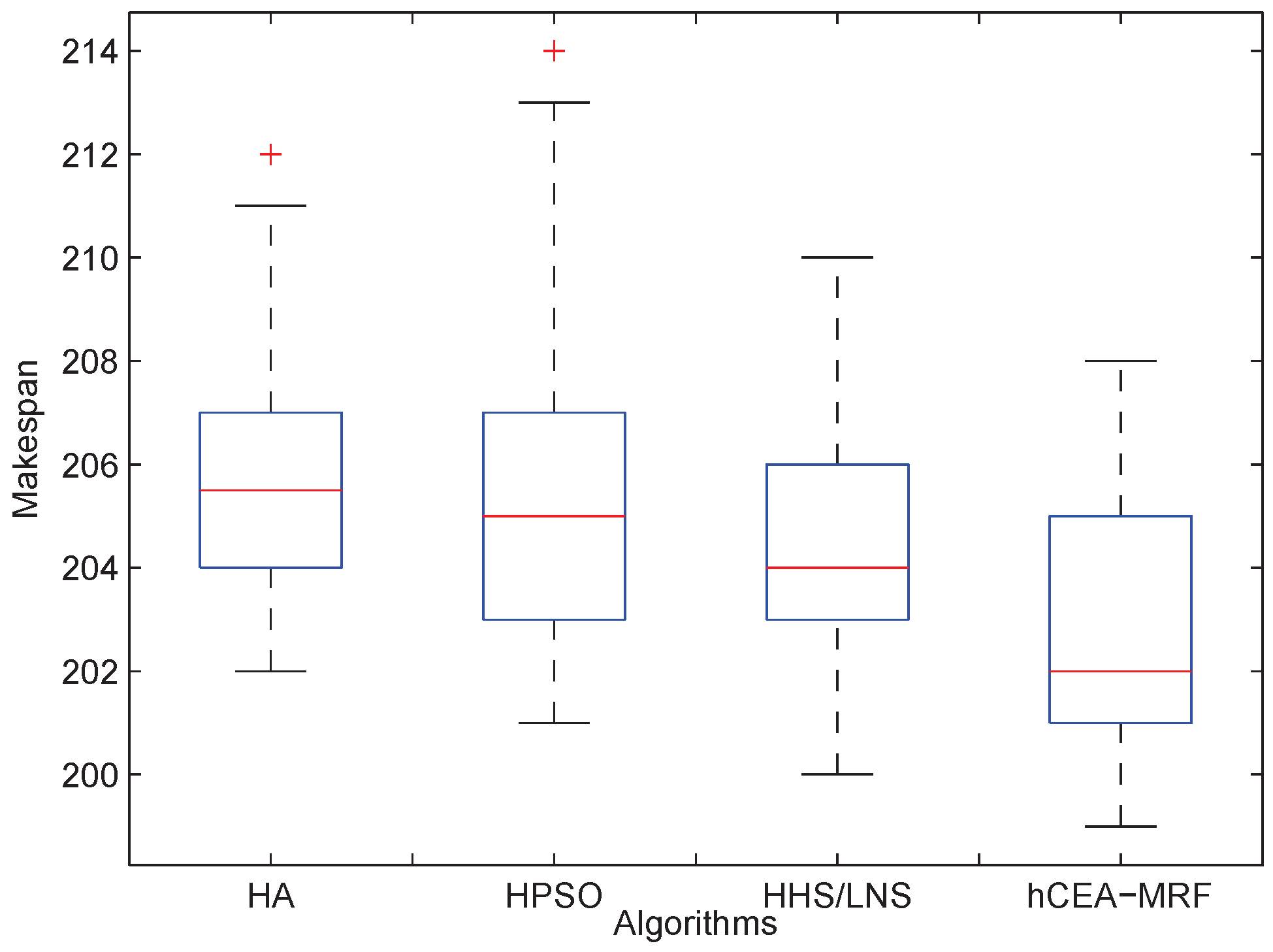
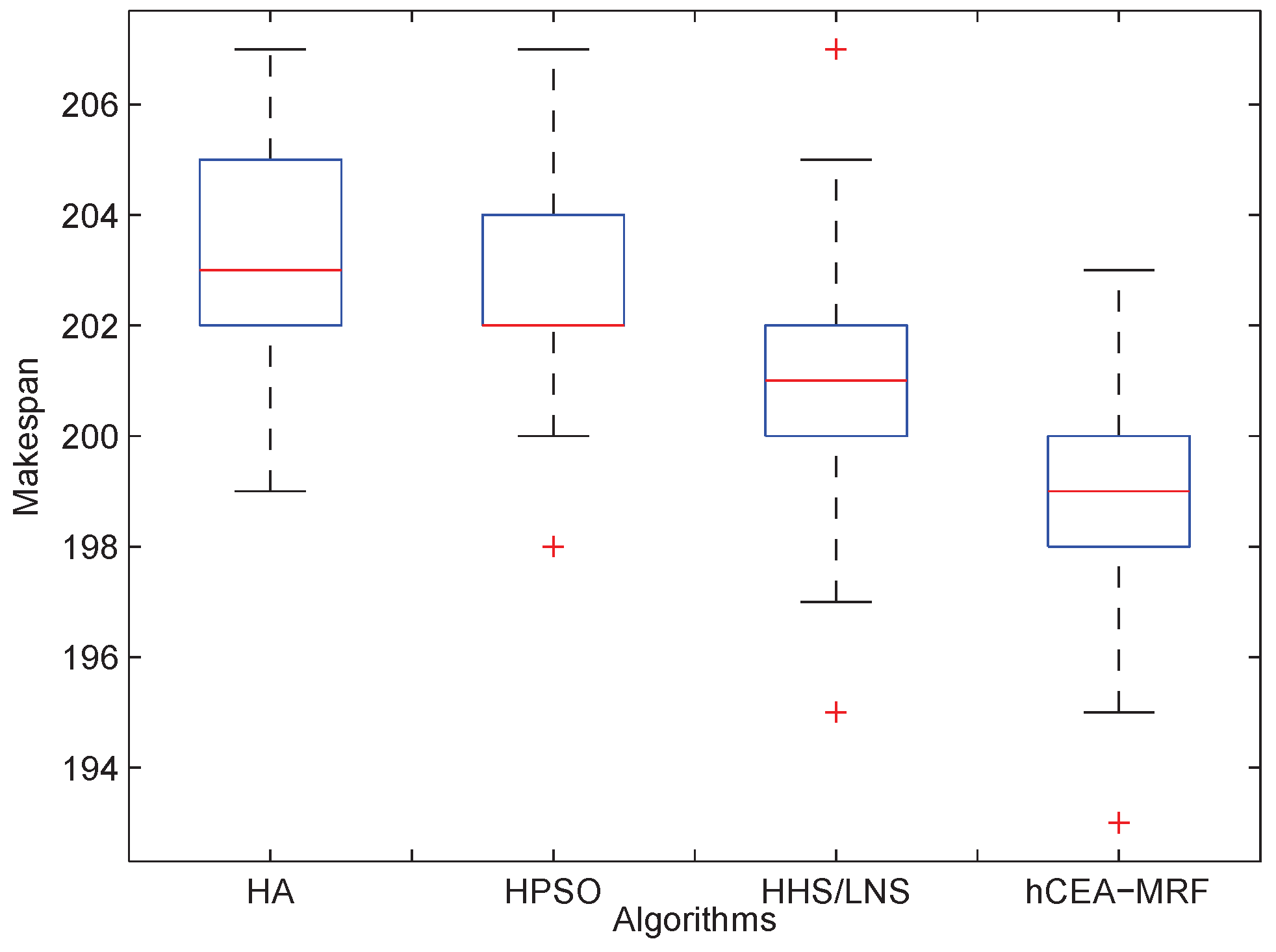
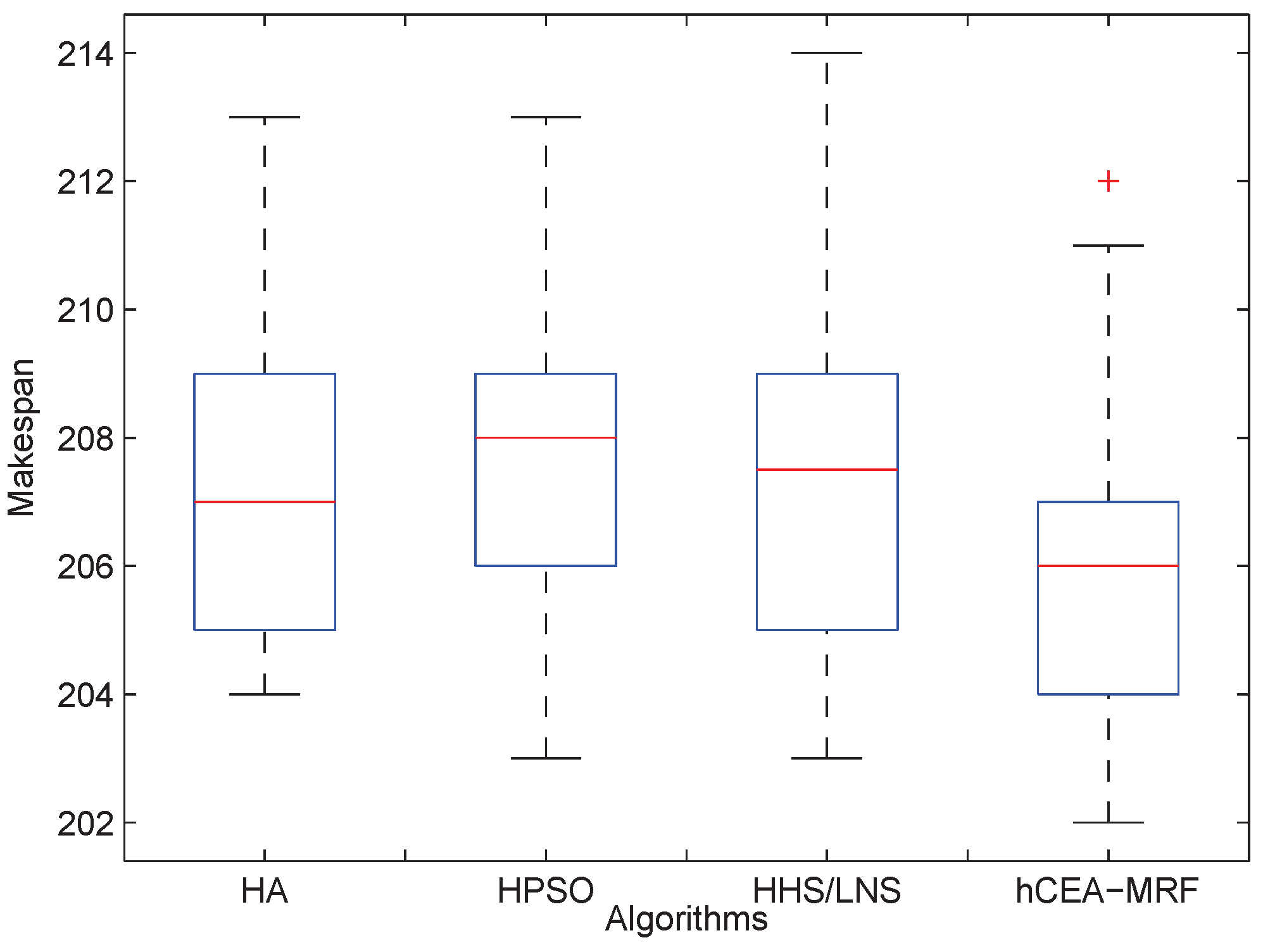
4.2.2. Stability Compared with State-of-the-Art

We record the makespan of 30 scenarios of UMk10, GMk10 and EMk10. The box plots are listed in Figure 6, Figure 7 and Figure 8, respectively. We can see that our proposed hCEA-MRF has better stability with the following aspects. The minimum value, medium value and maximum value obtained by our hCEA-MRF are all better than the state-of-the-art ones. The box of hCEA-MRF is narrower than the state-of-the-art ones.

4.3. Discussion of hCEA-MRF

4.3.1. Effect of the Self-Adaptive Parameter Strategy

In order to verify the effectiveness of self-adaptive parameter strategy, we compared our proposed self-adaptive parameter strategy with two widely applied self-adaptive parameter strategies, i.e, the linear increase strategy and the linear decrease strategy. We called our hCEA-MRF with the linear increase and the linear decrease self-adaptive parameter strategies hCEA-MRF(I) and hCEA-MRF(D), respectively. The instances generated by all three probability distributions are used for testing the effectiveness of our proposed algorithm. The experiments’ results are recorded in

Table 7. The performance of different parameter self-adaptive strategies for the generated instances by uniform distribution.

	hCEA-MRF(I)		hCEA-MRF(D)		hCEA-MRF
	Average	Variance	Average	Variance	Average	Variance
UMk01	40.4	2.7	40.5	2.47	39.8	1.9
UMk02	26.8	2.1	26.9	1.7	25.9	1.4
UMk03	208.4	48.7	209.1	47.2	205.2	41.1
UMk04	61.8	2.4	62.1	2.1	60.8	1.7
UMk05	173.5	6.5	174.1	5.8	171.1	4.6
UMk06	61.1	2.8	60.6	3.1	58.6	3.7
UMk07	141.3	12.7	140.7	13.1	138.4	11.8
UMk08	535.7	110.4	530.9	113.2	522.3	101.7
UMk09	310.8	170.4	308.4	167.1	302.3	156.9
UMk10	202.4	7.9	203.2	5.6	198.8	4.6

,

Table 8. The performance of different parameter self-adaptive strategies for the generated instances by Gaussian distribution.

	hCEA-MRF(I)		hCEA-MRF(D)		hCEA-MRF
	Average	Variance	Average	Variance	Average	Variance
GMk01	42.1	3.4	42.6	2.9	40.7	2.3
GMk02	27.4	2.1	26.9	1.7	26.3	1.9
GMk03	207.5	48.7	207.5	46.5	206.4	44.7
GMk04	63.1	2.5	62.6	2.9	61.6	2.3
GMk05	175.6	6.3	174.7	5.7	173.2	5.5
GMk06	62.1	4.9	61.7	5.2	60.1	4.5
GMk07	143.2	13.8	142.5	13.1	141.4	12.9
GMk08	527.4	106.4	526.4	105.6	524.6	104.8
GMk09	304.5	164.3	305.2	163.3	303.5	162.4
GMk10	203.4	7.6	204.3	8.4	202.8	6.8

and

Table 9. The performance of different parameter self-adaptive strategies for the generated instances by exponential distribution.

	hCEA-MRF(I)		hCEA-MRF(D)		hCEA-MRF
	Average	Variance	Average	Variance	Average	Variance
EMk01	44.3	3.8	43.6	3.5	42.3	3.1
EMk02	29.3	3.2	28.4	3.2	27.2	2.5
EMk03	209.4	44.7	208.4	43.5	207.2	43.2
EMk04	64.3	3.1	63.7	2.8	62.1	2.7
EMk05	175.6	7.4	174.5	6.9	173.2	6.5
EMk06	63.6	3.4	63.9	2.8	62.1	2.3
EMk07	142.3	14.6	141.8	13.6	140.2	13.2
EMk08	527.4	104.5	525.3	103.8	524.5	103.2
EMk09	305.4	160.2	304.8	159.4	303.5	158.4
EMk10	206.4	6.3	207.5	6.3	205.8	5.9

, respectively. We can see that our proposed self-adaptive parameter strategy performs better than two compared strategies. The reason is that the compared strategies only self-adjust according to the iterations of algorithms but take no performance into consideration. However, our proposed strategy not only considers the information of iteration but also considers the performance of different update equations. Thus, our proposed strategy performs better.

4.3.2. Effect of the Decomposition Strategy

In order to verify the effectiveness of MRF-based decomposition strategy, we compared our proposed MRF-based decomposition strategy with two effective and lower computational cost decomposition strategies, i.e, fixed decomposition and set-based decomposition strategy. We named our hCEA-MRF with fixed decomposition and set-based decomposition strategies hCEA-MRF(F) and hCEA-MRF(S), respectively. The experiments’ results of the instances with three probability distributions are recorded in

Table 10. The performance of different decomposition strategies for the generated instances by uniform distribution.

	hCEA-MRF(F)		hCEA-MRF(S)		hCEA-MRF
	Average	Variance	Average	Variance	Average	Variance
UMk01	43.2	3.2	41.7	2.3	39.8	1.9
UMk02	27.3	2.5	26.4	2.1	25.9	1.4
UMk03	208.4	43.2	206.6	42.5	205.2	41.1
UMk04	62.1	2.4	61.8	2.2	60.8	1.7
UMk05	174.2	6.8	172.8	5.4	171.1	4.6
UMk06	63.2	4.9	61.7	4.2	58.6	3.7
UMk07	142.5	13.1	140.5	12.3	138.4	11.8
UMk08	528.8	109.3	526.4	103.5	522.3	101.7
UMk09	308.1	164.4	305.2	160.9	302.3	156.9
UMk10	206.4	4.5	204.5	5.2	198.8	4.6

,

Table 11. The performance of different decomposition strategies for the generated instances by Gaussian distribution.

	hCEA-MRF(F)		hCEA-MRF(S)		hCEA-MRF
	Average	Variance	Average	Variance	Average	Variance
GMk01	44.3	3.5	43.6	3.1	40.7	2.3
GMk02	28.4	2.7	27.6	2.5	26.3	1.9
GMk03	209.5	46.8	207.4	45.6	206.4	44.7
GMk04	63.2	3.5	62.8	2.8	61.6	2.3
GMk05	175.6	6.7	174.9	6.5	173.2	5.5
GMk06	63.2	5.8	62.1	5.6	60.1	4.5
GMk07	144.2	14.6	143.1	13.7	141.4	12.9
GMk08	527.5	106.4	529.4	105.7	524.6	104.8
GMk09	306.4	164.3	305.8	163.5	303.5	162.4
GMk10	206.3	7.8	205.6	7.2	202.8	6.8

and

Table 12. The performance of different decomposition strategies for the generated instances by exponential distribution.

	hCEA-MRF(F)		hCEA-MRF(S)		hCEA-MRF
	Average	Variance	Average	Variance	Average	Variance
EMk01	44.3	3.8	43.7	2.8	42.3	3.1
EMk02	29.5	4.3	28.3	3.5	27.2	2.5
EMk03	209.6	46.3	208.3	45.3	207.2	43.2
EMk04	64.2	3.7	63.2	3.1	62.1	2.7
EMk05	176.6	7.9	175.3	7.3	173.2	6.5
EMk06	65.3	4.5	63.8	3.6	62.1	2.3
EMk07	143.9	15.4	142.2	14.8	140.2	13.2
EMk08	526.8	106.4	525.2	104.2	524.5	103.2
EMk09	306.6	161.5	205.8	160.9	303.5	158.4
EMk10	207.8	7.5	206.5	6.9	205.8	5.9

, respectively. We can see that our proposed decomposition strategy performs better than the two compared strategies. This is because our proposed MRF-based decomposition strategy takes the correlation among variables into consideration instead of relying on the random technique. Meanwhile, our proposed MRF-based decomposition strategy has lower computational cost as discussed in the previous section.

5. Conclusions

Flexible job shop scheduling is an important research issue and is widely applied in many real-world applications as well. However, the stochastic factors are usually ignored and are not considered. In this paper, we modeled the stochastic processing times with three distribution probabilities. We proposed a hybrid cooperative co-evolution algorithm with Markov random field (MRF)-based decomposition strategy for solving the stochastic flexible scheduling problem with the objective to minimize the expectation and the standard variance of makespan. Various simulation experiments are constructed and the simulation results demonstrate the validity of hCEA-MRF. The reasons are that the MRF-based decomposition strategy considers the correlation among variables instead of relying on a random technique and the self-adaptive parameter strategy adjusts the parameters based on the performance and fitness instead of the random technique as well.

References

1. Jiang, T.; Zhang, C.; Zhu, H. Energy-Efficient Scheduling for a Job Shop Using an Improved Whale Optimization Algorithm. Mathematics 2018, 6, 220. [Google Scholar] [CrossRef]
2. Gur, S.; Eren, T. Scheduling and Planning in Service Systems with Goal Programming: Literature Review. Mathematics 2018, 6, 265. [Google Scholar] [CrossRef]
3. Kim, J.S.; Jeon, E.; Noh, J.; Park, J.H. A Model and an Algorithm for a Large-Scale Sustainable Supplier Selection and Order Allocation Problem. Mathematics 2018, 6, 325. [Google Scholar] [CrossRef]
4. Gao, S.; Zheng, Y.; Li, S. Enhancing strong neighbour-based optimization for distributed model predictive control systems. Mathematics 2018, 6, 86. [Google Scholar] [CrossRef]
5. Zamani, A.G.; Zakariazadeh, A.; Jadid, S. Day-ahead resource scheduling of a renewable energy based virtual power plant. Appl. Energy 2016, 169, 324–340. [Google Scholar] [CrossRef]
6. Wang, C.N.; Le, T.M.; Nguyen, H.K. Application of optimization to select contractors to develop strategies and policies for the development of transport infrastructure. Mathematics 2019, 7, 98. [Google Scholar] [CrossRef]
7. Zhan, Z.; Liu, X.; Gong, Y.; Zhang, J.; Chung, H.S.-H.; Li, Y. Cloud computing resource scheduling and a survey of its evolutionary approaches. ACM Comput. Surv. (CSUR) 2015, 47, 63. [Google Scholar] [CrossRef]
8. Montoya-Torres, J.R.; Franco, J.L.; Isaza, S.N.; Jimenez, H.F.; Herazo-Padilla, N. A literature review on the vehicle routing problem with multiple depots. Comput. Ind. Eng. 2015, 79, 115–129. [Google Scholar] [CrossRef]
9. Ccalics, B.; Bulkan, S. A research survey: Review of AI solution strategies of job shop scheduling problem. J. Intell. Manuf. 2015, 26, 961–973. [Google Scholar] [CrossRef]
10. Lin, L.; Gen, M. Hybrid evolutionary optimisation with learning for production scheduling: State-of-the-art survey on algorithms and applications. Int. J. Prod. Res. 2018, 56, 193–223. [Google Scholar] [CrossRef]
11. Chaudhry, I.A.; Khan, A.A. A research survey: Review of flexible job shop scheduling techniques. Int. Trans. Oper. Res. 2016, 23, 551–591. [Google Scholar] [CrossRef]
12. Ouelhadj, D.; Petrovic, S. A survey of dynamic scheduling in manufacturing systems. J. Sched. 2009, 12, 417. [Google Scholar] [CrossRef]
13. Lei, D. Simplified multi-objective genetic algorithms for stochastic job shop scheduling. Appl. Soft Comput. 2011, 11, 4991–4996. [Google Scholar] [CrossRef]
14. Hao, X.; Gen, M.; Lin, L.; Suer, G.A. Effective multiobjective EDA for bi-criteria stochastic job-shop scheduling problem. J. Intell. Manuf. 2017, 28, 833–845. [Google Scholar] [CrossRef]
15. Kundakci, N.; Kulak, O. Hybrid genetic algorithms for minimizing makespan in dynamic job shop scheduling problem. Comput. Ind. Eng. 2016, 96, 31–51. [Google Scholar] [CrossRef]
16. Zhang, R.; Wu, C. An artificial bee colony algorithm for the job shop scheduling problem with random processing times. Entropy 2011, 13, 1708–1729. [Google Scholar] [CrossRef]
17. Zhang, R.; Song, S.; Wu, C. A two-stage hybrid particle swarm optimization algorithm for the stochastic job shop scheduling problem. Knowl.-Based Syst. 2012, 27, 393–406. [Google Scholar] [CrossRef]
18. Azadeh, A.; Negahban, A.; Moghaddam, M. A hybrid computer simulation-artificial neural network algorithm for optimisation of dispatching rule selection in stochastic job shop scheduling problems. Int. J. Prod. Res. 2012, 50, 551–566. [Google Scholar] [CrossRef]
19. Horng, S.; Lin, S.-H.; Yang, F.-Y. Evolutionary algorithm for stochastic job shop scheduling with random processing time. Expert Syst. Appl. 2012, 39, 3603–3610. [Google Scholar] [CrossRef]
20. Gu, J.; Gu, X.; Gu, M. A novel parallel quantum genetic algorithm for stochastic job shop scheduling. J. Math. Anal. Appl. 2009, 355, 63–81. [Google Scholar] [CrossRef]
21. Nguyen, S.; Zhang, M.; Johnston, M.; Tan, K.C. Automatic design of scheduling policies for dynamic multi-objective job shop scheduling via cooperative coevolution genetic programming. IEEE Trans. Evol. Comput. 2014, 18, 193–208. [Google Scholar] [CrossRef]
22. Gu, J.; Gu, M.; Cao, C.; Gu, X. A novel competitive co-evolutionary quantum genetic algorithm for stochastic job shop scheduling problem. Comput. Oper. Res. 2010, 37, 927–937. [Google Scholar] [CrossRef]
23. Horng, S.-C.; Lin, S.-S. Two-stage Bio-inspired Optimization Algorithm for Stochastic Job Shop Scheduling Problem. Int. J. Simul. Syst. Sci. Technol. 2015, 16, 4. [Google Scholar] [CrossRef]
24. Mei, Y.; Li, X.; Yao, X. Cooperative coevolution with route distance grouping for large-scale capacitated arc routing problems. IEEE Trans. Evol. Comput. 2014, 18, 435–449. [Google Scholar] [CrossRef]
25. Ghasemishabankareh, B.; Li, X.; Ozlen, M. Cooperative coevolutionary differential evolution with improved augmented Lagrangian to solve constrained optimisation problems. Inf. Sci. 2016, 369, 441–456. [Google Scholar] [CrossRef]
26. Ma, X.; Li, X.; Zhang, Q.; Tang, K.; Liang, Z.; Xie, W.; Zhu, Z. A Survey on Cooperative Co-evolutionary Algorithms. IEEE Trans. Evol. Comput. 2018. [Google Scholar] [CrossRef]
27. Qi, Y.; Bao, L.; Ma, X.; Miao, Q.; Li, X. Self-adaptive multi-objective evolutionary algorithm based on decomposition for large-scale problems: A case study on reservoir flood control operation. Inf. Sci. 2016, 367, 529–549. [Google Scholar] [CrossRef]
28. Omidvar, M.N.; Li, X.; Mei, Y.; Yao, X. Cooperative co-evolution with differential grouping for large scale optimization. IEEE Trans. Evol. Comput. 2014, 18, 378–393. [Google Scholar] [CrossRef]
29. Li, X. Decomposition and cooperative coevolution techniques for large scale global optimization. In Proceedings of the Companion Publication of the 2014 Annual Conference on Genetic and Evolutionary Computation, Vancouver, BC, Canada, 12–16 July 2014; pp. 819–838. [Google Scholar] [CrossRef]
30. Sun, Y.; Kirley, M.; Li, X. Cooperative Co-evolution with Online Optimizer Selection for Large-Scale Optimization. In Proceedings of the Genetic and Evolutionary Computation Conference, Kyoto, Japan, 15–19 July 2018. [Google Scholar] [CrossRef]
31. Potter, M.A.; De Jong, K.A. A cooperative coevolutionary approach to function optimization. In Proceedings of the International Conference on Parallel Problem Solving from Nature, Jerusalem, Israel, 9–14 October 1994; pp. 249–257. [Google Scholar] [CrossRef]
32. Van, D.B.; Frans Engelbrecht, A.P. A cooperative approach to particle swarm optimization. IEEE Trans. Evol. Comput. 2004, 8, 225–239. [Google Scholar] [CrossRef]
33. Yang, Z.; Tang, K.; Yao, X. Large scale evolutionary optimization using cooperative coevolution. Inf. Sci. 2008, 178, 2985–2999. [Google Scholar] [CrossRef]
34. Mahdavi, S.; Rahnamayan, S.; Shiri, M.E. Multilevel framework for large-scale global optimization. Soft Comput. 2017, 21, 4111–4140. [Google Scholar] [CrossRef]
35. Chen, W.; Weise, T.; Yang, Z.; Tang, K. Large-scale global optimization using cooperative coevolution with variable interaction learning. In Proceedings of the International Conference on Parallel Problem Solving from Nature, Krakov, Poland, 11–15 September 2010; pp. 300–309. [Google Scholar] [CrossRef]
36. Sun, L.; Yoshida, S.; Cheng, X.; Liang, Y. A cooperative particle swarm optimizer with statistical variable interdependence learning. Inf. Sci. 2012, 186, 20–39. [Google Scholar] [CrossRef]
37. Hu, X.-M.; He, F.-L.; Chen, W.-N.; Zhang, J. Cooperation coevolution with fast interdependency identification for large scale optimization. Inf. Sci. 2017, 381, 142–160. [Google Scholar] [CrossRef]
38. Omidvar, M.N.; Yang, M.; Mei, Y.; Li, X.; Yao, X. DG2: A faster and more accurate differential grouping for large-scale black-box optimization. IEEE Trans. Evol. Comput. 2017, 21, 929–942. [Google Scholar] [CrossRef]
39. Sun, Y.; Kirley, M.; Halgamuge, S.K. A recursive decomposition method for large scale continuous optimization. IEEE Trans. Evol. Comput. 2017. [Google Scholar] [CrossRef]
40. Van Haaren, J.; Davis, J. Markov Network Structure Learning: A Randomized Feature Generation Approach. In Proceedings of the Twenty-Sixth AAAI Conference on Artificial Intelligence, Toronto, ON, Canada, 22–26 July 2012; pp. 1148–1154. [Google Scholar]
41. Shakya, S.; Santana, R.; Lozano, J.A. A markovianity based optimisation algorithm. Genet. Programm. Evol. Mach. 2012, 13, 159–195. [Google Scholar] [CrossRef]
42. Sun, L.; Wu, Z.; Liu, J.; Xiao, L.; Wei, Z. Supervised spectral–spatial hyperspectral image classification with weighted markov random fields. IEEE Trans. Geosci. Remote Sens. 2015, 53, 1490–1503. [Google Scholar] [CrossRef]
43. Li, C.; Wand, M. Combining markov random fields and convolutional neural networks for image synthesis. In Proceedings of the IEEE Conference on Computer Vision and Pattern Recognition, Las Vegas, NV, USA, 27–30 June 2016; pp. 2479–2486. [Google Scholar]
44. Paragios, N.; Ramesh, V. A mrf-based approach for real-time subway monitoring. In Proceedings of the 2001 IEEE Computer Society Conference on Computer Vision and Pattern Recognition, CVPR 2001, Kauai, HI, USA, 8–14 December 2001. [Google Scholar] [CrossRef]
45. Tombari, F.; Stefano, L. 3D data segmentation by local classification and markov random fields. In Proceedings of the International Conference on 3DIMPVT, Hangzhou, China, 16–19 May 2011; pp. 212–219. [Google Scholar] [CrossRef]
46. Li, X.; Gao, L. An effective hybrid genetic algorithm and tabu search for flexible job shop scheduling problem. Int. J. Prod. Econ. 2016, 174, 93–110. [Google Scholar] [CrossRef]
47. Nouiri, M.; Bekrar, A.; Jemai, A.; Niar, S.; Ammari, A.C. An effective and distributed particle swarm optimization algorithm for flexible job-shop scheduling problem. J. Intell. Manuf. 2015, 1–13. [Google Scholar] [CrossRef]
48. Yuan, Y.; Xu, H. An integrated search heuristic for large-scale flexible job shop scheduling problems. Comput. Oper. Res. 2013, 40, 2864–2877. [Google Scholar] [CrossRef]
49. Brandimarte, P. Routing and scheduling in a flexible job shop by tabu search. Ann. Oper. Res. 1993, 41, 157–183. [Google Scholar] [CrossRef]
Figure 1. Illustration of random-key based representation.
Mathematics 07 00318 g001
Figure 2. Illustration of the machine assignment process.
Mathematics 07 00318 g002
Figure 3. Gantt chart of the illustrated solution for the instance in Table 3.
Mathematics 07 00318 g003
Figure 4. Illustration of the network structure of MRF.
Mathematics 07 00318 g004
Figure 5. The factors for X 1 , X 2 and X 3 for 100 samples.
Mathematics 07 00318 g005
Figure 6. Box plot for makespan conducted on UMk10.
Mathematics 07 00318 g006
Figure 7. Box plot for makespan conducted on GMk10.
Mathematics 07 00318 g007
Figure 8. Box plot for makespan conducted on EMk10.
Mathematics 07 00318 g008