1. Introduction
Wireless Sensor Networks (WSN) are relevant system architectures that can be applied in a wide range of applications [
1], from monitoring to tracking, visual surveillance, ranging also in many fields from industrial automation to agricultural systems, and target localization, both in military and civil sectors [
2].
Currently, WSN are becoming much more important because the senors’ computational capabilities are growing, and thus, many in-network tasks can be performed. It has been noticed that processing the information inside the network is faster and safer than sending raw data to the final user [
3]. Such in-network processing can drastically reduce the total computational time required after sensing tasks with a direct impact on power consumption [
4].
The network complex dynamics created by these in-network operations can be suitably managed by means of evolutionary optimization techniques [
5]. For instance, the problem of sensor lifetime maximization has been successfully approached in [
6] by means of genetic algorithms and in [
7] with genetical swarm optimization. The problem of coverage in WSN has been solved in [
8] with both the genetic algorithm and ant colony optimization. Another important problem of WSN, routing, has been widely approached by several authors: in [
9], a specific energy protocol has been designed to improve the network lifetime, while in [
10], it has been solved with genetical swarm optimization and in [
11] with particle swarm optimization.
The problem of task and resource allocation is a crucial problem in many frameworks. It is aimed at finding the optimal distribution of the tasks inside the network itself with reference to a specific goal. In the case of the deployment of multiple sensor devices with batteries, a fundamental goal is to maximize the total network lifetime, in other words to minimize the total energy consumption [
12]. In many WSN applications, the computational time is also a key parameter in the optimization process. Scheduling and planning have been already faced with evolutionary computation algorithms, like the genetic algorithm [
13], particle swarm optimization [
14], and ant colony optimization [
15]. In standard planning problems, these techniques have been demonstrated to have performances comparable with other deterministic optimization techniques [
16].
With recent advancements in massive parallel computing technologies, the problem of scheduling resources and tasks, for example in multiprocessor systems, is becoming more and more attractive. In this scenario, soft computing techniques represent a useful tool that can be effectively applied in task allocation optimization problems.
This work is based on a multi-hop network in which a set of tasks for parallel computing should be performed. The tasks are distributed and collected by a central node. By properly choosing the number of such processed tasks for each sensor, it is possible to change the total processing time and the network lifetime.
The analyzed task allocation problem is devoted to the minimization of the elaboration cycle time of the entire network, i.e., the total time required by the network to process all the tasks. The optimization is performed fixing a predefined scheduling protocol for each sensor and taking into consideration energy constraints expressed in terms of network lifetime.
To perform this optimization, a promising evolutionary optimization algorithm, named Social Network Optimization (SNO) [
17], has been used. SNO is a recently-developed population-based algorithm: in the literature, it has been applied to antenna optimization [
18], with a comparison between SNO and PSO; it has been also applied to model parameter matching problems [
19].
In order to assess SNO performance on task allocation, in this paper, the final results are compared with the solutions obtained by the following algorithms: Biogeography-Based Optimization (BBO), Differential Evolutionary (DE), the Genetic Algorithm (GA), Particle Swarm Optimization (PSO), and the Stud-Genetic Algorithm (SGA).
The paper is structured as follows:
Section 2 provides an overview of related works, and
Section 3 contains a description of the WSN with all the hypothesis and parameters adopted.
Section 4 provides a brief description of the optimization algorithm.
Section 5 reports the results of the optimization and the comparison. Finally, in
Section 6, some conclusions are drawn.
2. Related Works
Evolutionary optimization algorithms have been widely applied to optimization problems related to wireless sensor networks. The task assignments of WSN essentially aims to save energy, reducing the expenditure among the allocations and prolonging the network lifetime. Some authors had already proposed energy-efficiency approaches based on a mix of entropy theory and evolutionary computation theory [
20].
Moreover, the same problem has been also addressed by means of several evolutionary algorithms: for example, in [
21], task scheduling in heterogeneous distributed systems was evaluated comparing a multi-objective evolutionary algorithm with a hybrid genetic algorithm. Previously, genetic algorithms had been used in [
22] for a similar purpose, performing tests on a Java scheduler with a homogeneous set of processors. Additionally, in [
23], the authors proposed three different hybridizations between BBO and DE for the problem of power allocation in sensor networks.
Particle swarm optimization has been widely applied in WSN: the work in [
24] provided a wide review of these applications. As concerns the specific problem of task allocation, in [
25], the authors applied the PSO to the this problem with a particular concern regarding the network reliability. In [
26], the authors proposed the PSO in task optimization for tracking, showing that the heuristic algorithm can compete and win against deterministic approaches to the same problem. More recently, in [
27], a logic-based evolutionary algorithm compared to a binary PSO has been applied again to task allocation in WSN.
Social network optimization has been preliminary applied to task allocation in WSN [
28], but in this previous work, the scheduling algorithm was only partially considered and no energy constraints were included. Additionally, no comparison with other assessed evolutionary algorithms was proposed in order to validate SNO performance over the task allocation problem. In the present paper, all these aspects have been added, as clarified in the following sections.
3. Description of Wireless Sensor Networks
The analyzed problem in this paper is the tasks’ resource allocation in wireless sensor networks [
29].
The WSN is a system composed of a set of smart sensor devices, deployed in space, which can sense, process, send, and receive data. The communication adopts a multi-hop scheme for managing the signal-to-noise ratio without drastically compromising the global lifetime. Moreover, this structure can handle specific environmental constraints.
The most important node in the network is the cluster head: this node is devoted to transmission and reception of the data. It is in charge of splitting and gathering the data between the network nodes, and it cannot perform any further processing activity.
All the other standard nodes can be operated in four different modes:
computing mode: this is the phase related to the elaboration of the assigned task;
Reception (RX) mode: all the nodes can receive information from their neighbors;
Transmission (TX) mode: when a sensor is in this mode, it is transmitting the information to its predecessor in the network;
idle state: this is when a sensor is not performing any activity; in this state, the energy consumption is drastically reduced.
Thus, the sensors can be only in one of these four states and cannot perform more than one activity at the same time. On the other hand, the cluster head is devoted only to TX and RX operations. Due to this design option, it is equipped with a multi-input and multi-output transmission capability.
The sensor units can differ one from another in terms of processing speed, while the transmission rate is homogeneously distributed among all the nodes. This is justified due to the fact that, while the transmission rate is related to the signal frequency, the units can be different or can be set with different energy levels to improve the network lifetime.
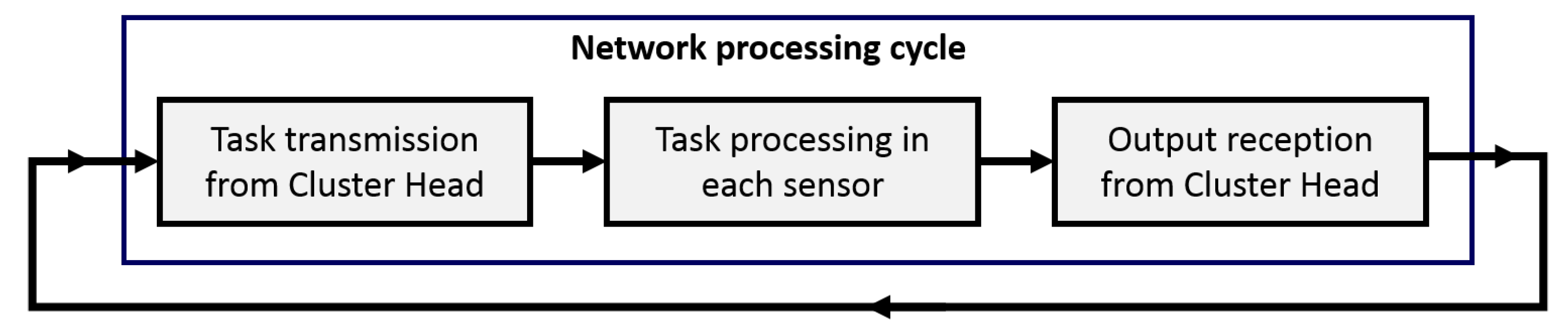
The specific selected application, namely the parallel computing field, imposes some constraints. Firstly, all the tasks require almost the same computational effort; for the sake of simplicity, in this paper, they have been considered equal. Moreover, a process cycle of the entire network consists of the transmission of the tasks from the cluster head to the sensors, the following elaboration, and in the final collection of the processed outputs. The following cycle can start only when all the outputs are collected, as represented in
Figure 1.
The scheduling process of this network is assumed to be in the first-in-first out (FIFO) logic. This control scheme has been selected because of its simplicity; even if it is not optimal by itself, it is part of the optimization process, so this sub-optimality can be reduced or eliminated. This logic has the advantages of being simple and can be implemented in the sensors, and it is valid for any kind of job the units should perform. Moreover, this logic is robust to some variation in the elaboration time of the other units.
Within this network, two aspect have been considered: the total cycle time and the network lifetime. The first is the maximum of the time required by the sensors:
On the other hand, the network lifetime is the number of cycles before the most stressed node ends its energy.
The total time required by the
sensor unit is the sum of the time spent in each of the four possible states:
where
is the total time required by the
unit,
is its elaboration time,
is its receiving time,
is its transmission time, and
is its idle time.
These times are all a function of the number of allocated tasks to each unit. Firstly, the processing time can be expressed as:
where
is the number of allocated tasks to the
unit,
is the number of Kilo Clock Cycles (KCC) required for elaborating one task, and
is its elaboration speed in KCC/s.
The time spent in reception mode depends on the network configuration, and it has two contributions: the time required for receiving the tasks from its predecessor and the time for receiving the output of the elaborations from reachable units (in graph theory, the set of reachable nodes is the set of nodes connected directly or indirectly to the analyzed node):
where
is the number of reachable units from the
sensor,
is the information amount sent from the cluster head to the nodes to assign a task,
is the output number of bits for each assigned task, and
is the reception speed.
The transmission time can be calculated with a very similar logic as the reception time. Nonetheless, it can be calculated in an easier way as a function of the reception time: in fact, it is the time for retransmitting the received information and to transmit the output of the task processed by the unit:
where
is the transmission speed. The transmission and the reception speed can be different because the transmission requires also the amplification of the signal.
The waiting time evaluation depends on the specific schedule of the activities and thus cannot be expressed as the other times, but it can be calculated at each simulation run of the network.
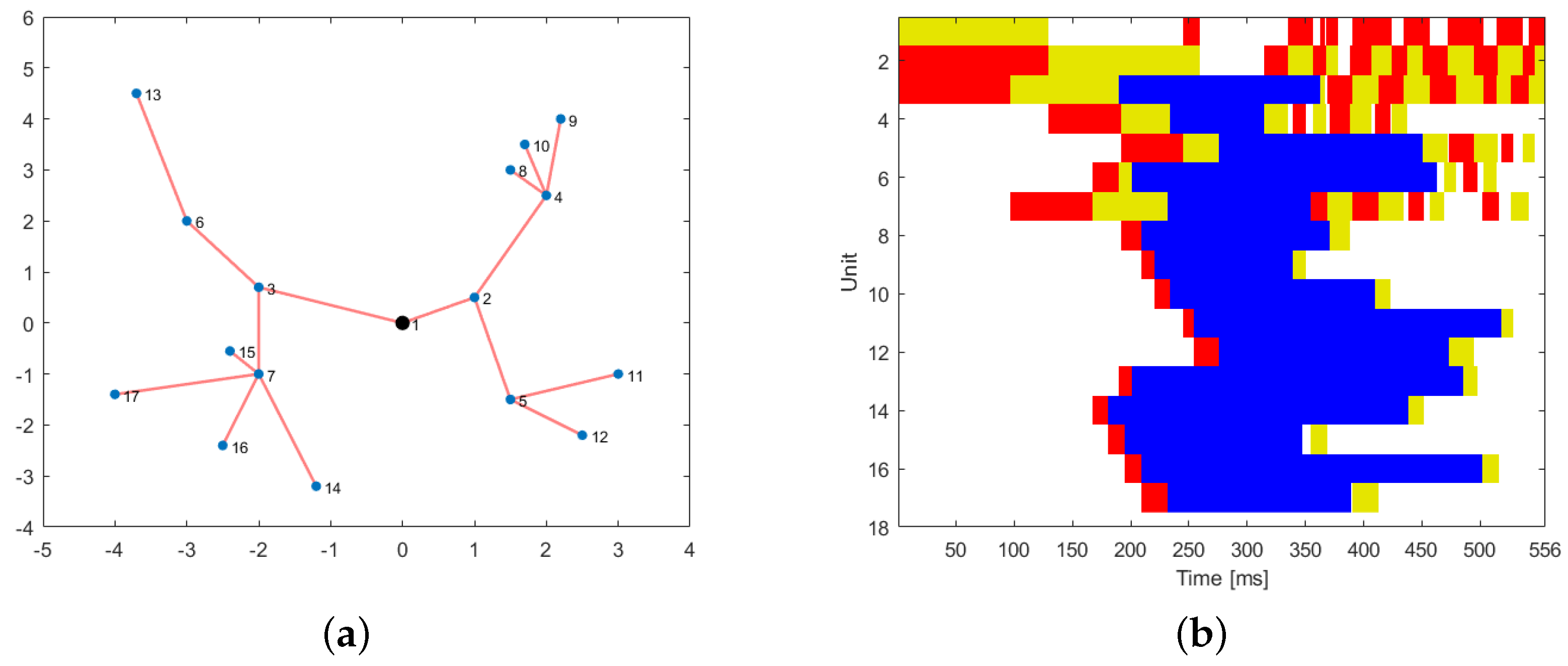
The scheduling is based on the following rules. The information is transmitted from the cluster head to the nodes, giving priority to the nodes with more subsequent nodes; when a node has finished the reception and the hopping of the information, it starts its elaboration; then, it sends back the information to its predecessorif it is in idle mode. Finally, it turns to idle mode for the information.
An example of the scheduling is proposed in
Figure 2.
As concerns the energy consumption, the following model has been applied. The sensors are fed by batteries with a total capacity of 9 kJ. The energy consumed is composed of four terms:
The first term is the energy for the communication. It is a function of the total number of bit transmitted and received (
):
where
is the energy required to maintain the communication equipment.
The amplification energy is required to have an acceptable signal-to-noise ratio. The transmission energy required by node
i to transmit to node
j depends on the number of transmitted bits (
) and on the transmission distance (
):
The elaboration energy depends on the elaboration time:
Finally, the energy consumed in idle time is considered negligible with respect to the other terms.
The network has been implemented in MATLAB; the parameters adopted in the simulation of the network are summarized in
Table 1.
4. Social Network Optimization
The optimization algorithm used in this paper is Social Network Optimization (SNO). It is a novel population-based algorithm that takes its inspiration from the information-sharing process in online social networks [
30]. The algorithm has already been applied to other engineering problems in which its effectiveness has been proven [
17].
The performances of this algorithm are very good in many engineering application problems, both in terms of convergence speed and reliability of the solution, and this makes the algorithm very suitable for facing the problem complexity in an affordable time [
31].
The basic element of SNO is the social network itself (
). It is a network of users (
) that communicates by means of posts (
):
Each user is characterized by a set of
opinions (
) (the bold means that it is a vector), its personal growth (
), a list of friends (
), and a reputation value for the other users of the social network (
):
The interaction between users takes place among two preferential paths: the first one is a friend network, where the connections between users are very strong and reciprocal, and a trust network, where the connections are weaker and monodirectional. Among these paths, the information is exchanged by means of posts: the information content is presented by a status containing the opinions of the user on the discussion topics.
The topic represents, out of the social metaphor, the possible design variables, while the status is the value assigned to them by each post that represents a candidate solution.
Each post contains the status,
, the name (the ID) of the user that has posted it (
), the time at which it was posted
, and a visibility value (
), that is, out of the metaphor, the cost value associated with each candidate solution by means of the objective function. Posts with high visibility are more likely to be seen by the other users, and thus can influence more individuals. The post visibility affects the reputation list: in fact, if the visibility of a post of the user
v is higher than the average, its reputation
grows, while if it is lower than the average, the reputation diminishes.
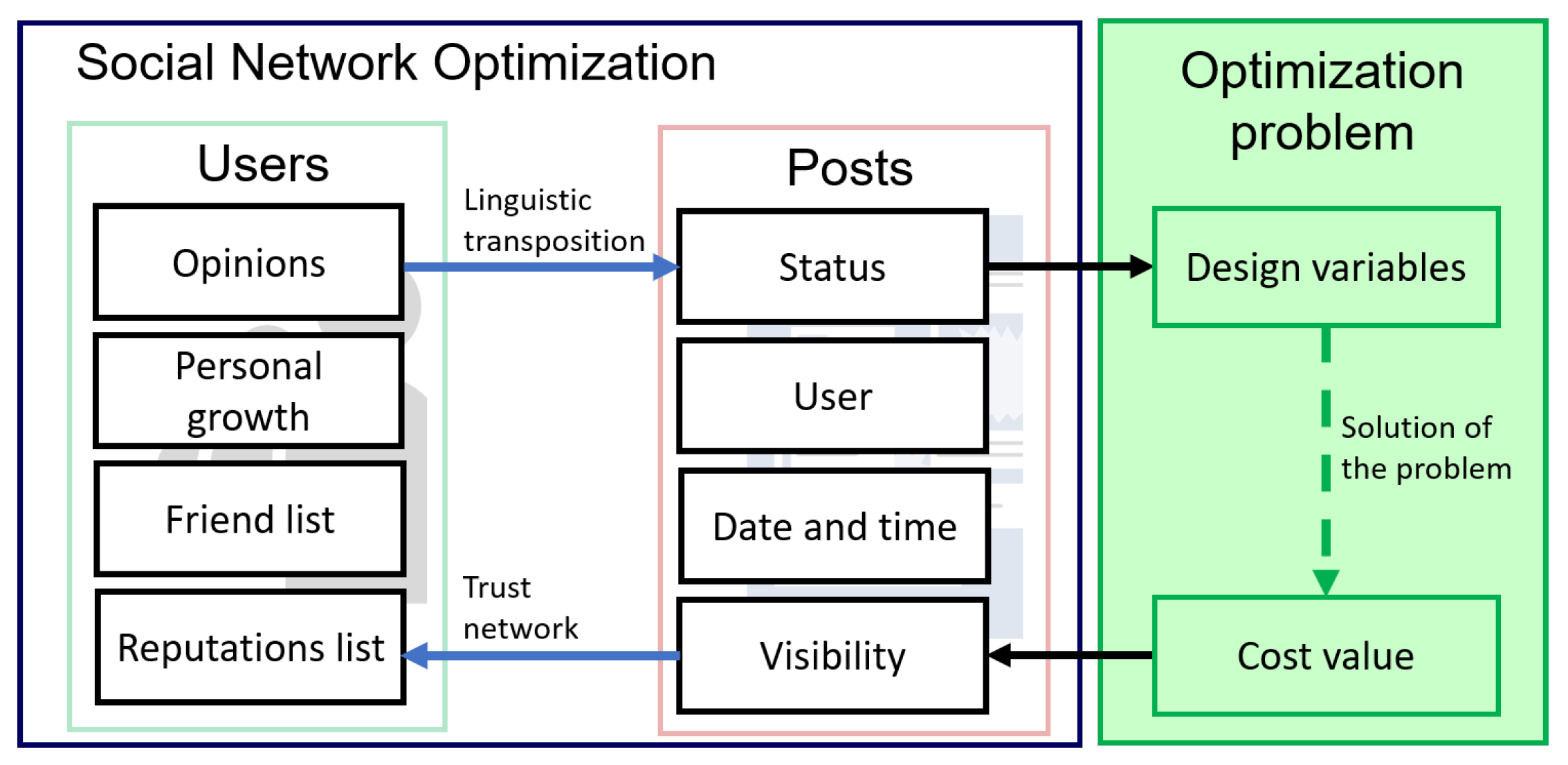
The opinions of a user are related o the corresponding status by means of the
linguistic transposition of the ideas. In SNO, it is modeled as a random variable with zero mean and a small standard deviation.
Figure 3 is representative of the basic structure of social network optimization and of its relation with a generic optimization problem.
All the above presented structures evolve with time. There are two basic mechanisms in this evolution: the personal growth of individuals and the modification of the friend and trust networks.
The personal growth can be represented by the variation of the opinions with time:
The user change
is based on the complex contagion model of idea diffusion:
where
is the attracting idea created in the interaction process;
and
are two user-defined parameters that represent the inclination of each user to change his/her idea.
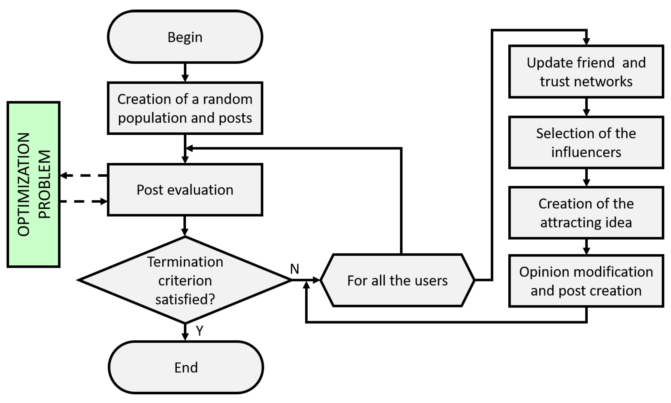
The attracting idea is created by means of the friend and trust networks. In fact, each user selects some influencers in these networks by means of a rank selection based on the visibility value. Then, the identified posts are combined with a crossover operator to create the attracting idea. The networks’ evolutions are intrinsically different. The friend network evolves by means of the process of recommendation, so a user v has a probability of becoming a friend of a user u that is proportional to the number of common friends. On the other hand, the friendship can be eliminated when the number of common friends becomes low. Furthermore, the trust network is based on the reputation value: all the individuals that for the user u have a reputation higher than a predefined threshold belong to its trust network.
The time evolution of the structures of SNO is described in the flowchart of
Figure 4.
5. Optimization Problem: Description and Results
The described wireless sensor network represents the engineering problem to which social network optimization has been here applied. In the following, the optimization problem is formalized, and the results are presented.
5.1. Problem Description
The optimization problem is the following one:
subject to:
is the design variable vector (the number of tasks associated with each sensor), and is the design variable space. The minimization function is the maximum cycle time, i.e., the time required by the slowest sensor in the network.
There are two constraints that were introduced: the first one ensures that all the tasks are managed by the network, while the second one that the network lifetime lasts more than 4000 cycles.
This problem has been codified in SNO by means of a candidate solution represented by a vector of
N elements, where
N is the number of sensors, and each of them can range from 0–1. The first constraint has been managed with a proper decodification of the candidate solution. In fact, it is possible to process the candidate solution
in the following way:
In this way, the produced vector is composed only by an integer. On the other hand, it is not ensured that the sum is equal to . To fix this aspect, the missing task () are calculated and assigned to the first sensors.
The management of the second constraint has been done with a penalty approach. This means that the actual visibility value for the optimizer is:
where
is the lifetime of the network expressed in elaboration cycles and
is the Heaviside function defined as:
This penalty definition has been selected because it ensures that a solution that satisfies the constraints has a cost value greater than a good solution. It has been decided to not further penalize the solutions because they can have good features that could help the convergence process.
In the following, the optimization process has been performed firstly without taking this last constraint into consideration, and then considering it. In both cases, firstly, the results obtained by means of SNO are presented, and then it is compared with other algorithms.
The algorithms adopted for the comparison are the following:
Biogeography-Based Optimization (BBO), implemented starting from [
32] and modified to improve the exploration;
Differential Evolutionary (DE) [
33];
Genetic Algorithm (GA) [
34], implemented for the real value objective function, with single-point crossover and non-linear rank-based selection;
Particle Swarm Optimization (PSO) [
35], with variable inertia and velocity constraints;
Stud-Genetic Algorithm (SGA) [
36], an effective variation of GA in which one of the parents is always the best individual in the population and the second one is selected with a rank-based selection.
For all these algorithms, the population was set to 20 individuals (this value was obtained from a parametric analysis performed on standard benchmarks [
37]), and the termination criterion was set to 5000 objective function evaluations. In all the tests, 100 independent trials were performed to have statistical reliability of the results.
5.2. Results of Unconstrained Optimization
The first optimization set of trials was done without the constraint on the minimum lifetime. Firstly, the results of SNO are presented, and then, they are compared with the results of the other algorithms.
5.2.1. Social Network Optimization Results
SNO has been used to find an optimal solution of the WSN task allocation problem.
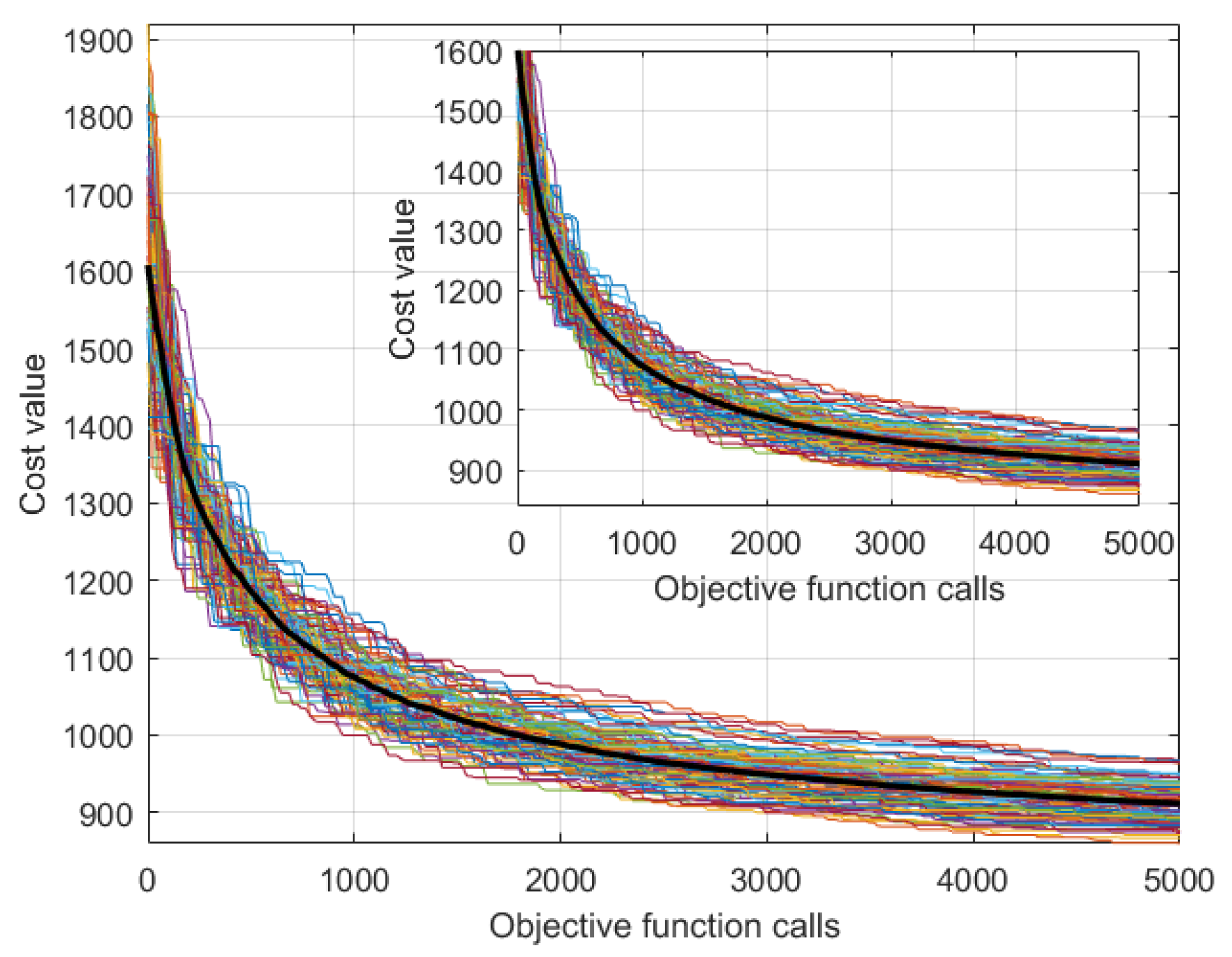
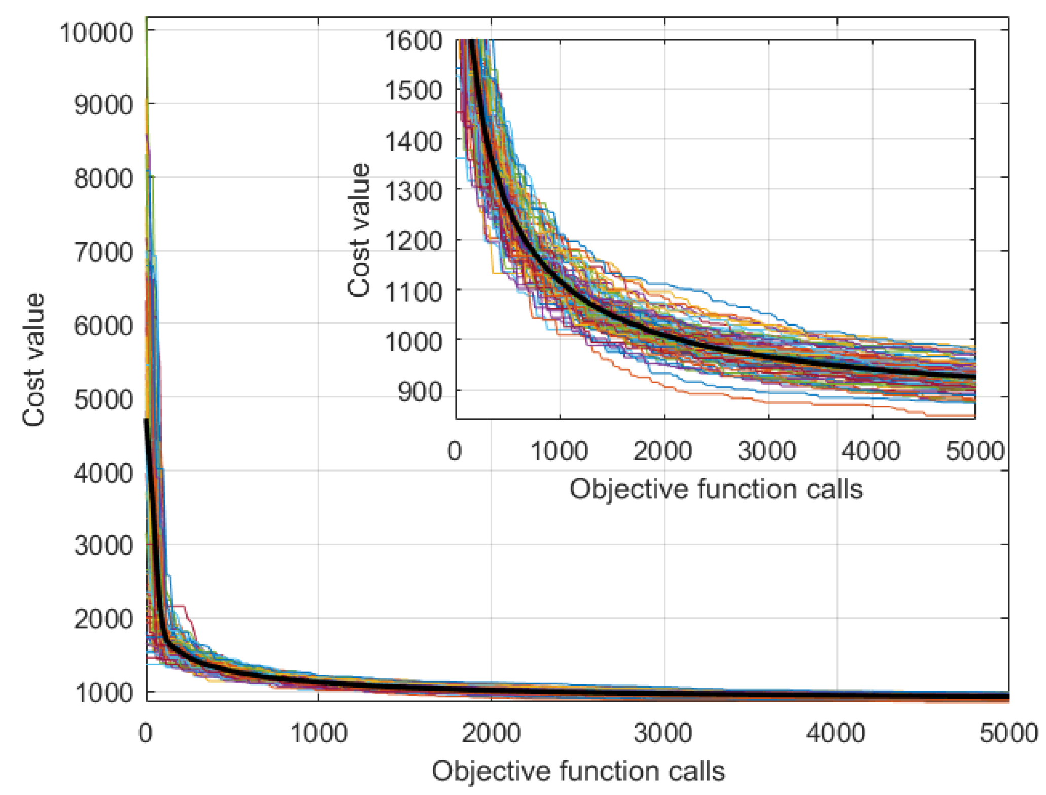
Figure 5 shows the convergence curves of the 100 independent trials. The small plot is a zoom of the convergence curves limiting the cost value to 1600.
The convergence curves have a very similar behavior, showing the robustness of the algorithm. All the trials were able to find solutions with the cost value below 1000.
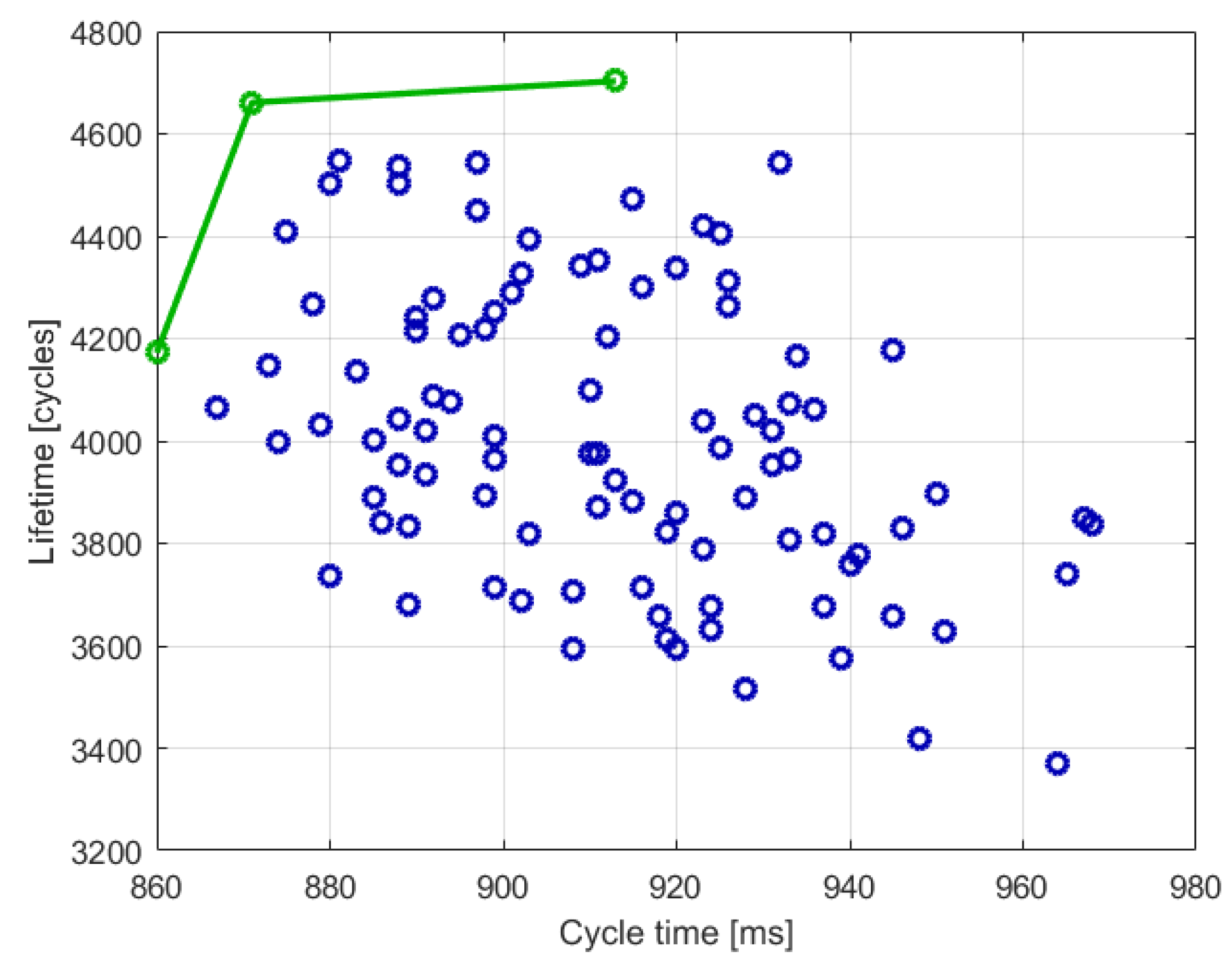
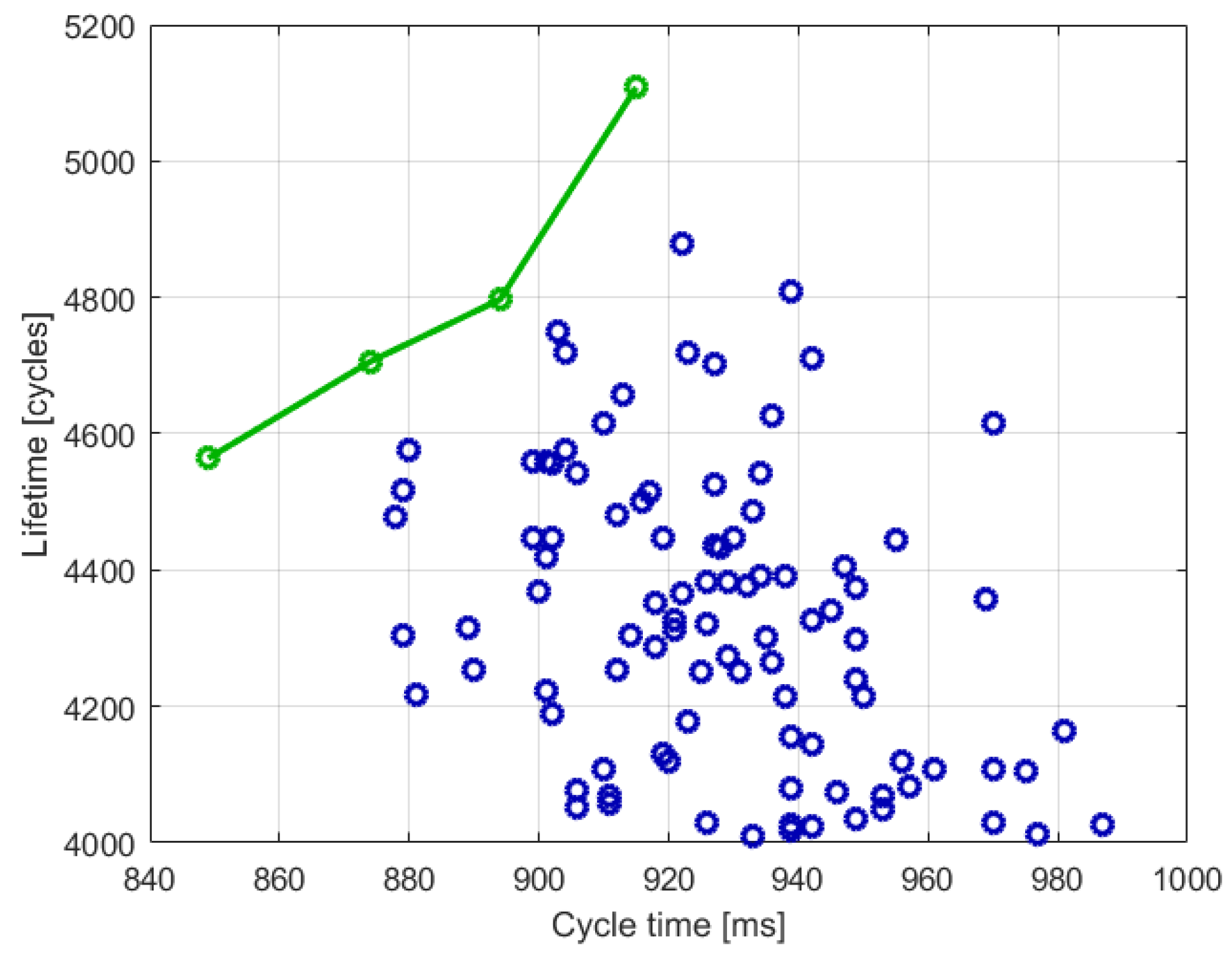
It is possible to represent the obtained solutions in a plane in which the horizontal axis is the maximum cycle time (in milliseconds) and the vertical axis is lifetime (in elaboration cycles).
Figure 6 shows the 100 optimal values obtained by SNO. The three green dots are the Pareto front. In this case, it is possible to notice that many solutions have a lifetime below 4000 cycles. All these solutions will be discarded in the constrained optimization.
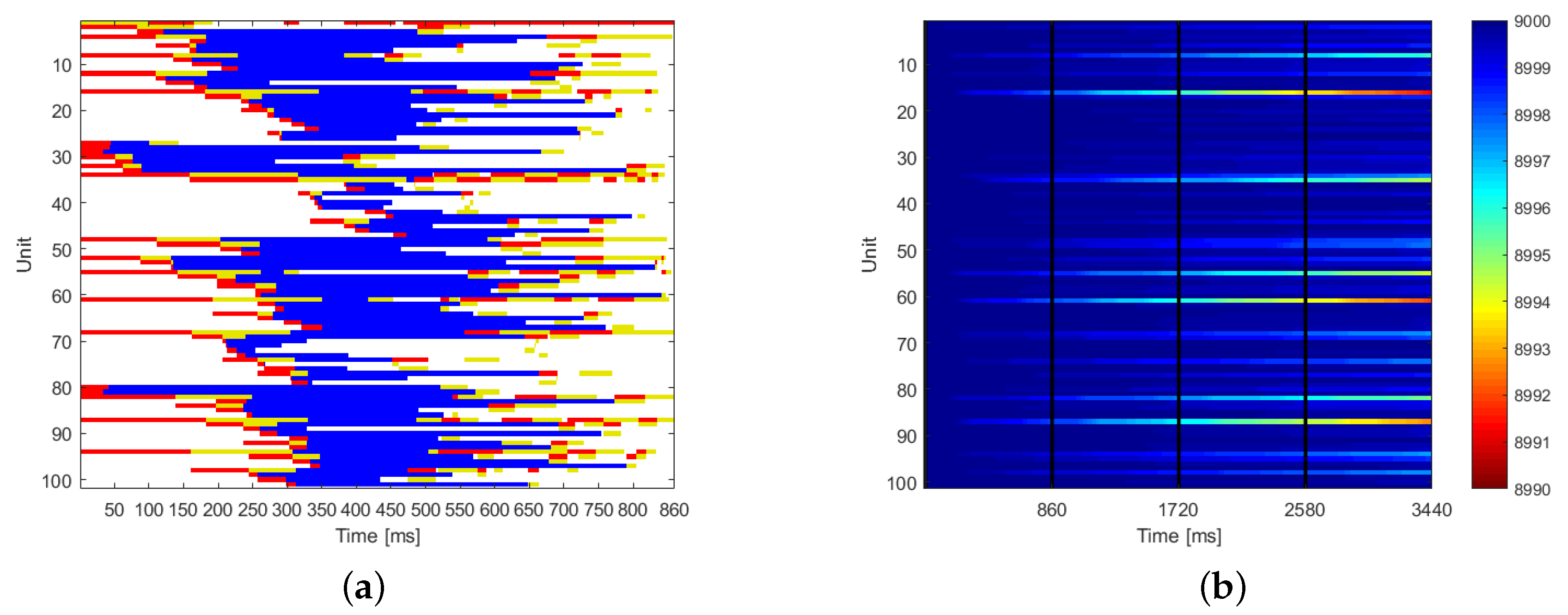
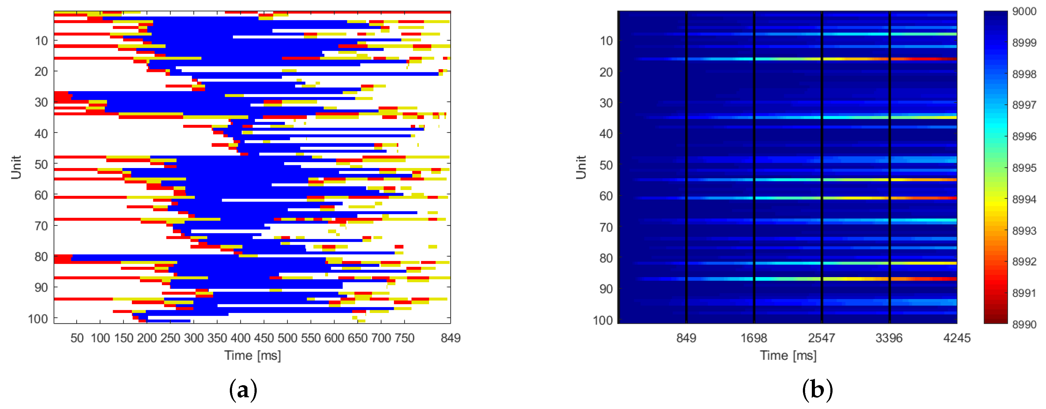
The optimal scheduling of one elaboration cycle is represented in
Figure 7a. The red color represents the receiving mode, the blue the elaboration status, and the yellow the transmitting mode. White color is the idle status.
Figure 7b shows the energy content of all the sensors during the first five elaboration cycles. The black vertical lines show the end of each cycle. The color is representative of the energy content: blue means full of charge.
5.2.2. Comparison between SNO and Other Algorithms
In this section, the comparison between SNO and the other optimization algorithms is presented.
Table 2 shows the results of the six algorithms: the mean value is the average optimal result obtained in the 100 independent trials; the minimum value is the best solution; and the last column is the results of a
t-test with the significance level at 5%: if SNO is better, the value of the
t-test is “+”; if the two algorithms are equal, it is “0”, or if SNO is the worst, the value is “−”.
It is possible to see that SNO outperformed four out of the five algorithms and that only Stud-GA had similar performances. In particular, Stud-GA is able to find a better best solution, while the average results of the two algorithms are almost the same.
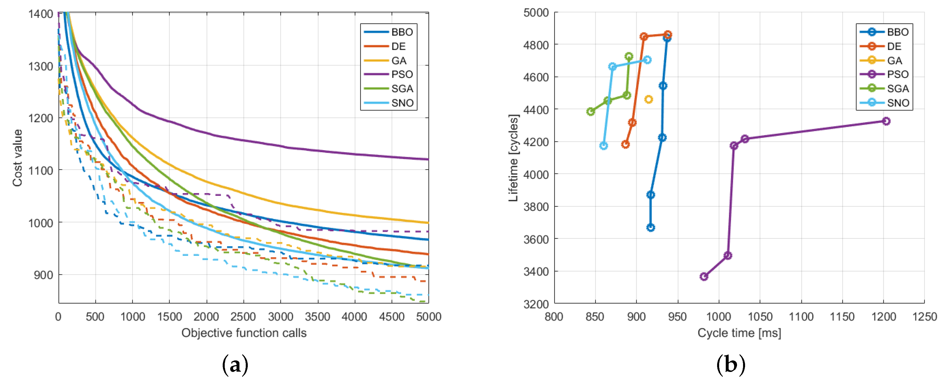
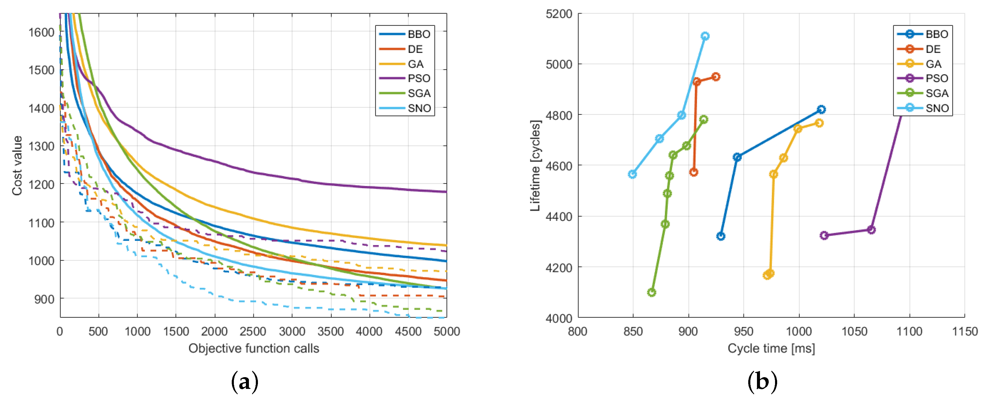
Figure 8a shows a comparison in terms of convergence curves: the continuous line is the average convergence, while the dashed line is the best trial.
Figure 8b shows a comparison of the Pareto front: in this figure, it is possible to notice that the results of SNO are much better than the results of the other algorithms.
The convergence of Stud-GA is slower than the one of SNO at the beginning of the optimization process, while it is able to reach a comparable result at the end. On the other hand, BBO has a very good initial convergence, but then the convergence rate drastically diminishes.
5.3. Results of Constrained Optimization
Here, the results of the constrained optimization are presented. As has been done before, firstly, the results of SNO and then the comparison are presented.
5.3.1. Social Network Optimization Results
Figure 9 shows the convergence curves of the 100 independent trials. Here, the zoom is important to see the good convergence of the trials and the low standard deviation. Also in this case, it is possible to notice that all the results had a cost value below 1000.
With respect to the curves of the unconstrained optimization, it is possible to see that the initial values have a very high cost. This is due to the fact that the solutions found violate the feasibility constraint. After a few iterations, the algorithm is able to bring all the solutions within the feasibility limits, and then, the convergence rate becomes similar to the unconstrained optimization.
As done previously, it is possible to represent the obtained solutions as the maximum cycle time–lifetime plane.
Figure 10 shows the 100 optimal values obtained by SNO. The four green dots are the Pareto front.
The optimal scheduling of one elaboration cycle is represented in
Figure 11a, while
Figure 11b shows the energy levels of the sensors in the first five elaboration cycles.
Comparing these results with the ones of the unconstrained optimization, it is possible to see that, here, the cycle time is lower. Comparing the two schedules, the solutions are very similar. On the other hand, the energy consumption is more distributed among the sensors.
5.3.2. Comparison between SNO and Other Algorithms
In this section, the comparison between SNO and the other optimization algorithms is presented.
Table 3 shows the results of the six algorithm: the mean value is the average optimal result obtained in the 100 independent trials; the minimum value is the best solution; and the last column is the results of a
t-test with the significance level at 5%.
Figure 12a shows a comparison in terms of convergence curves: the continuous line is the average convergence, while the dashed line is the best trial.
Figure 12b shows a comparison of the Pareto front: in this figure, it is possible to notice that the results of SNO are much better than the ones of the other algorithms.
6. Conclusions
In this paper, the task allocation problem in WSN has been faced: the integrated use of evolutionary techniques can optimize and enhance these systems, both in terms of energy efficiency and computationally efficiency.
The optimization algorithm used in this paper is a recently-developed algorithm called social network optimization: this algorithm has been applied in two different problems. The first one is represented by an unconstrained optimization, while the second is a constrained problem.
The obtained results have been compared with other well-established algorithms. The results show that SNO is able to obtain very good results if compared with the other algorithms. In particular, the convergence of SNO is more effective, especially at dealing with the constrained problem.
Future developments of this work can be focused more on the robustness of the WSN communication process: in fact, it is possible to take also into account failures in the information exchange between sensors. This can have an impact on both the total cycle time and the final energy consumption.


