Estimating the Expected Discounted Penalty Function in a Compound Poisson Insurance Risk Model with Mixed Premium Income

Abstract

In this paper, we consider an insurance risk model with mixed premium income, in which both constant premium income and stochastic premium income are considered. We assume that the stochastic premium income process follows a compound Poisson process and the premium sizes are exponentially distributed. A new method for estimating the expected discounted penalty function by Fourier-cosine series expansion is proposed. We show that the estimation is easily computed, and it has a fast convergence rate. Some numerical examples are also provided to show the good properties of the estimation when the sample size is finite.

1. Introduction

In this paper, we consider an insurance risk model with mixed premium income defined by

$$\begin{array}{c}U\left(t\right)=u+ct+\sum _{i=1}^{M\left(t\right)}{Y}_i-\sum _{j=1}^{N\left(t\right)}{X}_j,t\ge 0,\end{array}$$

(1)

where $u\ge 0$ is the initial surplus, $c\ge 0$ is the constant premium rate, and $U\left(t\right)$ denotes the surplus level of an insurance company at time t. The premium number process $M\left(t\right)$ and the claim number process $N\left(t\right)$ are homogenous Poisson processes with intensity $\mu >0$ and $\lambda >0$, respectively. The individual claim sizes, $X_1,X_2,\dots$, are positive independent and identically distributed (i.i.d) continuous random variables with density function f. The premium sizes, $Y_1,Y_2,\dots$ are positive i.i.d. continuous random variables with exponential distribution function $g\left(y\right)=\beta e^{-\beta y}$, $y,\beta >0$, where $\beta$ is unknown. Throughout this paper, we assume that ${\left\{M\left(t\right)\right\}}_{t\ge 0},{\left\{N\left(t\right)\right\}}_{t\ge 0},{\left\{X_i\right\}}_{i\ge 1}$ and ${\left\{Y_j\right\}}_{j\ge 1}$ are mutually independent.

Whenever the surplus process becomes negative, we say that ruin occurs. The ruin time is defined by

$$\tau =inf\{t\ge 0:U(t)<0\},$$

if for all $t\ge 0$, $U\left(t\right)>0$, we denote $\tau =\infty$. To avoid that ruin is a certain event, suppose that the following condition holds throughout this paper.

Net profit condition

$$c+\frac{\mu }{\beta }-\lambda \mathbb{E}\left[X\right]>0.$$

The above condition guarantees that the expectation of the surplus process will always be positive at any time $t>0$.

Let $\delta \ge 0$ be the interest force, defining the expected discounted penalty function by

$$\begin{array}{c}\Phi \left(u\right)=\mathbb{E}[e^{-\delta \tau }\mathrm{w}(U(\tau -),|U\left(\tau \right)\left|\right){\mathbf{1}}_{(\tau <\infty )}|U\left(0\right)=u],u\ge 0,\end{array}$$

(2)

where, $\mathrm{w}:[0,\infty )\times [0,\infty )\to [0,\infty )$ is a measurable penalty function of the surplus before ruin and the deficit at ruin, and ${\mathbf{1}}_A$ is an indicator function of the event A. This function was first introduced by Gerber and Shiu [1], and is called Gerber-Shiu function in the literature. It has become an important and standard risk measure in ruin theory since various quantities of interests in ruin theory can be obtained for different values of the discount factor $\delta$ and different penalty functions $\mathrm{w}$. For recent research progress on the Gerber-Shiu function, we can refer to work by Lin et al. [2], Yuen et al. [3,4], Zhao and Yin [5], Chi [6], Yin and Wang [7], Chi and Lin [8], Shen et al. [9], Yin and Yuen [10], Zhao and Yao [11], Li et al. [12,13], Dong et al. [14], and Wang and Zhang [15], among others.

For the classical insurance risk model, the premium rate is usually set to a constant. Extensive research has been done on the ruin measures of the model and its extension under the constant premium rate, such as ruin probability, Gerber-Shiu function (see, e.g., Gerber and Shiu [1], Willmot and Dickson [16], Wang et al. [17], Yin and Yuen [18], Dong and Yin [19], Yu [20], Yin et al. [21], Zeng et al. [22], Zhao et al. [23] and Yu et al. [24]). However, in the actual insurance business, the premium income of an insurance company, especially a small one, is sometimes volatile and random. In view of this situation, Boucherie et al. [25] first extended the classical risk model to the risk model with stochastic premium income by replacing the constant premium income with a compound Poisson process. Since then, the risk model with stochastic premium income has been widely studied by many scholars. The non-ruin probability and ruin probability were, respectively, studied by Boikov [26] and Temnov [27]. Bao [28], Bao and Ye [29] and Yang and Zhang [30] studied the Gerber-Shiu function in the classical risk model, delayed renewal risk model and Sparre Andersen risk model by assuming the premium process are Poisson process, respectively. Supposing premium and claim process follow compound Poisson processes, a defective renewal equation satisfied by the Gerber-Shiu function was established by Labbé and Sendova [31]. Yang and Zhang [32] further studied the above model by assuming that there exists a specific dependence structure among the claim sizes, inter-claim times and premium sizes and the individual premium sizes are exponentially distributed. Zhao and Yin [33] considered a renewal risk model where the premiums follow a compound Poisson risk process and the claims follow a generalized Erlang(n) process. The Laplace transform and a defective renewal equation for the Gerber-Shiu function are derived when the premium sizes are exponentially distributed. For more study on the risk model with stochastic premium income, the interested readers are referred to the work by Xu et al. [34], Yu [35,36], Zhou et al. [37], Gao and Wu [38], Zhou et al. [39], Deng et al. [40] and Zeng et al. [41] and the references therein.

The above-mentioned papers assume that some probability characteristics of the surplus process are known, however, which are usually unknown for an insurance company. Actually, some data information on the surplus process, such as surplus levels, claim and premium numbers, and claim and premium sizes, can be obtained. Thus, some semi-parametric and parametric estimations of the ruin probability and Gerber-Shiu function for different risk models are presented in recent literature (e.g., Politis [42], Wang and Yin [43], Yuen and Yin [44], Zhang et al. [45], Wang et al. [46], Zhang [47], Zhang and Yang [48,49] and Shimizu and Zhang [50], Peng and Wang [51,52], Yang et al. [53,54]). Besides, some effective methods, such as Laplace transform, Fourier-Sinc series expansion and Laguerre series expansion, have been applied in estimating the ruin probability and Gerber-Shiu function based on the observed data information. We refer the interested readers to Shimizu [55], Zhang [56], Zhang and Su [57,58] and Su et al. [59], among others.

In recent years, Fang and Oosterlee [60] proposed a novel method for pricing European options by Fourier-cosine series expansion, which is also called the COS method in the literature. It can be easily applied to approximate an integrable function as long as the corresponding Fourier transform has closed-form expression. Now, the COS method has been widely used for pricing options and other financial derivatives (see, e.g., Fang and Oosterlee [61] and Zhang and Oosterlee [62]). Recently, the COS method has also been used in risk theory to compute and estimate some risk measures by some actuarial researchers. For example, Chau et al. [63,64] used the COS method to compute the ruin probability and Gerber-Shiu function in the Lévy risk models. Zhang [65] applied the COS method to compute the density of the time to ruin in the classical risk model. Yang et al. [66] used a two-dimensional COS method to estimate the discounted density function of the deficit at ruin in the classical risk model with stochastic income where the premiums are only described by a compound Poisson process and the premium sizes are exponential distributed. Inspired by Yang et al. [66], in this paper, we extend the risk model of Yang et al. [66] by considering that there is also constant rate premium income process. Then, we use the COS method to estimate the expected discounted penalty function in this risk model with mixed premiums income process. The remainder of this paper is organized as follows. In Section 2, we first briefly introduce the Fourier-cosine series expansion method, and then derive the Fourier transform of the expected discounted penalty function. In Section 3, an estimator of the expected discounted penalty function is proposed by the observed sample of the surplus process. The consistent property is studied in Section 4 under large sample size setting. Finally, in Section 5, we present some simulation results to show that the estimator behaves well under finite sample size setting.

2. Preliminaries on Expected Discounted Penalty Function

2.1. Fourier-Cosine Series Expansion

In this subsection, we present some known results on the Fourier-cosine series expansion method. Let $L^1\left({\mathbb{R}}_{+}\right)$ denote the class of integrable functions on the positive axis, and let $\mathcal{F}f$ and $\mathcal{L}f$ denote the Fourier transform and Laplace transform of a $f\in L^1\left({\mathbb{R}}_{+}\right)$, respectively. For any complex number z, we denote its real part and imaginary part by $Re\left(z\right)$ and $Im\left(z\right)$, respectively.

It is known that an integrable function f defined on $[a_1,a_2]$ has the following cosine series expansion,

$$\begin{array}{c}f\left(x\right)=\sum _{k=0}^{\infty }{}^{\prime }\left\{\frac{2}{a_2-a_1}{\int }_{a_1}^{a_2}f\left(x\right)cos\left(k\pi \frac{x-a_1}{a_2-a_1}\right)dx\right\}cos\left(k\pi \frac{x-a_1}{a_2-a_1}\right),\end{array}$$

(3)

where ${\sum }^{\prime }$ means the first term of the summation has half weight. For a function $f\in L^1\left({\mathbb{R}}_{+}\right)$, we introduce an auxiliary function

$$\begin{array}{c}{f}_a\left(x\right)=f\left(x\right)·{\mathbf{1}}_{(0\le x\le a)},a>0,\end{array}$$

then $f_a$ has a finite domain $[0,a]$ and $f\left(x\right)=f_a\left(x\right)$ when $x\in [0,a]$. By Equation (3), we have

$$\begin{array}{c}f\left(x\right)=f_a\left(x\right)=\sum _{k=0}^{\infty }{}^{\prime }\left\{\frac{2}{a}{\int }_0^{a}f\left(x\right)cos\left(k\pi \frac{x}{a}\right)dx\right\}cos\left(k\pi \frac{x}{a}\right),0\le x\le a.\end{array}$$

(4)

For large a, we have

$$\begin{array}{c}\frac{2}{a}{\int }_0^{a}f\left(x\right)cos\left(k\pi \frac{x}{a}\right)dx=\frac{2}{a}Re\left\{{\int }_0^{a}f\left(x\right)e^{i\frac{k\pi }{a}x}dx\right\}\approx \frac{2}{a}Re\left\{\mathcal{F}f\left(\frac{k\pi }{a}\right)\right\},\end{array}$$

thus

$$\begin{array}{c}f\left(x\right)\approx \sum _{k=0}^{\infty }{}^{\prime }\frac{2}{a}Re\left\{\mathcal{F}f\left(\frac{k\pi }{a}\right)\right\}cos\left(k\pi \frac{x}{a}\right),0\le x\le a.\end{array}$$

Furthermore, for a large integer K, the above summation can be truncated as follows:

$$\begin{array}{c}f\left(x\right)\approx \sum _{k=0}^{K-1}{}^{\prime }\frac{2}{a}Re\left\{\mathcal{F}f\left(\frac{k\pi }{a}\right)\right\}cos\left(k\pi \frac{x}{a}\right),0\le x\le a.\end{array}$$

(5)

As for the expected discounted penalty function, it follows from Equation (5) that for $0\le u\le a$,

$$\begin{array}{c}\Phi \left(u\right)\approx {\Phi }_{K,a}\left(u\right):=\sum _{k=0}^{K-1}{}^{\prime }\frac{2}{a}Re\left\{\mathcal{F}\Phi \left(\frac{k\pi }{a}\right)\right\}cos\left(k\pi \frac{x}{a}\right).\end{array}$$

(6)

It can be easily seen that the key of approximating the expected discounted penalty function by Fourier-cosine series expansion method is to calculate the Fourier transform $\mathcal{F}\Phi \left(s\right)$ for $s\in \{\frac{k\pi }{a}:k=0,1,\dots ,K-1\}$. Therefore, we derive a specific expression of Fourier transform $\mathcal{F}\Phi (·)$ in the next section.

2.2. The Fourier Transform of Expected Discounted Penalty Function

In this subsection, we derive the Fourier transform of the expected discounted penalty function. For convenience, we introduce the Dickson-Hipp operator $T_s$ (see, e.g., Dickson and Hipp [67] and Li and Garrido [68]), which for any integrable function f on $(0,\infty )$ and any complex number s with $Re\left(s\right)\ge 0$ is defined as

$$T_{s}f\left(y\right)={\int }_y^{\infty }{e}^{-s(x-y)}f\left(x\right)dx={\int }_0^{\infty }{e}^{-sx}f(x+y)dx,y\ge 0.$$

The Dickson-Hipp operator has been widely used in ruin theory to simplify the expression of ruin related functions. For properties on this operator, we refer the interested readers to Li and Garrido [68].

We call the following equation (with respect to s) the Lundberg’s fundamental equation for the risk model defined in Equation (1),

$$\begin{array}{c}(\beta -s)\left[s-\frac{\delta +\mu +\lambda }{c}+\frac{\mu }{c}·\frac{\beta }{\beta -s}+\frac{\lambda }{c}\mathcal{L}f\left(s\right)\right]=0.\end{array}$$

(7)

By Lemma 2.1 in Zhao and Yin [33], we known that for $\delta \ge 0$ and $c>0$, the above equation has exactly two nonnegative roots, denoted as ${\rho }_1,{\rho }_2$ in this literature, and one of the roots ${\rho }_1$ equals 0 when $\delta =0$.

Remark 1.

Let

$$\begin{array}{c}\chi \left(s\right)=\delta +\mu +\lambda -cs-\lambda \mathcal{L}f\left(s\right)+\frac{\mu \beta }{s-\beta },s\ge 0.\end{array}$$

It is obvious that $\chi \left(s\right)=0$ also has exactly two nonnegative roots ${\rho }_1,{\rho }_2$. Under net profit condition, we have

$$\begin{array}{cc}{\chi }^{{}^{\prime }}\left(s\right)& =-c+\lambda {\int }_0^{\infty }x{e}^{-sx}f\left(x\right)dx-\frac{\mu \beta }{{(s-\beta )}^2}\hfill \\ & \le -c-\lambda \mathbb{E}\left[X\right]-\frac{\mu }{\beta }<0,0\le s<\beta ,\hfill \end{array}$$

which implies that $\chi \left(s\right)$ is decreasing on $[0,\beta )$. In addition, $\chi \left(s\right)$ is continuous on $[0,\beta )$, $\chi \left(0\right)=\delta \ge 0$ and $\chi (\beta -0)=-\infty$. Therefore, we conclude that the root ${\rho }_1$ of equation $\chi \left(s\right)=0$ is located in the interval $[0,\beta )$, and, in particular, ${\rho }_1=0$ when $\delta =0$; then, ${\rho }_2$ is located in the interval $(\beta ,\infty )$.

By Theorem 3.1 in Zhao and Yin [33], when stochastic premium income follows a compound Poisson process, we known that the expected discounted penalty function satisfies the following renewal equation

$$\begin{array}{c}\Phi \left(u\right)={\int }_0^u\Phi (u-x)H\left(x\right)dx+K\left(u\right),\end{array}$$

(8)

where

$$\begin{array}{c}H\left(x\right)=\frac{\lambda }{c}\left[\frac{\beta -{\rho }_1}{{\rho }_1-{\rho }_2}{T}_{{\rho }_1}f\left(x\right)+\frac{\beta -{\rho }_2}{{\rho }_2-{\rho }_1}{T}_{{\rho }_2}f\left(x\right)\right],\hfill \\ K\left(u\right)=\frac{\lambda }{c}\left[\frac{\beta -{\rho }_1}{{\rho }_1-{\rho }_2}{T}_{{\rho }_1}\omega \left(u\right)+\frac{\beta -{\rho }_2}{{\rho }_2-{\rho }_1}{T}_{{\rho }_2}\omega \left(u\right)\right],\hfill \\ \omega \left(u\right)={\int }_u^{\infty }\mathrm{w}(u,x-u)f\left(x\right)dx.\hfill \end{array}$$

To derive the Fourier transform of $\Phi \left(u\right)$, we assume the following condition holds true.

Condition 1. The penalty function $\mathrm{w}$ satisfies

$${\int }_0^{\infty }{\int }_0^{\infty }(1+x)\mathrm{w}(x,y)f(x+y)dydx<\infty .$$

This condition guarantees $\Phi \in L^1\left({\mathbb{R}}_{+}\right)$.

Now, we compute the Fourier transform of the expected discounted penalty function. Applying the Fourier transform on both sides of Equation (8) gives

$$\begin{array}{cc}\mathcal{F}\Phi \left(s\right)& ={\int }_0^{\infty }{e}^{isu}\Phi \left(u\right)du\hfill \\ & ={\int }_0^{\infty }{e}^{isu}{\int }_0^u\Phi (u-x)H\left(x\right)dxdu+{\int }_0^{\infty }{e}^{isu}K\left(u\right)du\hfill \\ & ={\int }_0^{\infty }{\int }_0^{\infty }{e}^{is(z+x)}\Phi \left(z\right)dzdx+\mathcal{F}K\left(s\right)\hfill \\ & =\mathcal{F}\Phi \left(s\right)\mathcal{F}H\left(s\right)+\mathcal{F}K\left(s\right),\hfill \end{array}$$

leading to

$$\begin{array}{c}\mathcal{F}\Phi \left(s\right)=\frac{\mathcal{F}K\left(s\right)}{1-\mathcal{F}H\left(s\right)}.\end{array}$$

(9)

For the Fourier transform $\mathcal{F}H\left(s\right)$, we have

$$\begin{array}{cc}\mathcal{F}H\left(s\right)& ={\int }_0^{\infty }{e}^{isu}H\left(x\right)dx=\frac{\lambda }{c}\left[\frac{\beta -{\rho }_1}{{\rho }_1-{\rho }_2}{\int }_0^{\infty }{e}^{isx}{T}_{{\rho }_1}f\left(x\right)dx+\frac{\beta -{\rho }_2}{{\rho }_2-{\rho }_1}{\int }_0^{\infty }{e}^{isx}{T}_{{\rho }_2}f\left(x\right)dx\right],\hfill \end{array}$$

where

$$\begin{array}{cc}{\int }_0^{\infty }{e}^{isu}{T}_{{\rho }_j}f\left(x\right)dx& ={\int }_0^{\infty }{e}^{isx}{\int }_x^{\infty }{e}^{-{\rho }_j(y-x)}f\left(y\right)dydx\hfill \\ & ={\int }_0^{\infty }{\int }_x^{\infty }{e}^{(is+{\rho }_j)x}·e^{-{\rho }_{j}y}f\left(y\right)dydx\hfill \\ & =\frac{1}{{\rho }_j+is}\left[{\int }_0^{\infty }{e}^{isy}f\left(y\right)dy-{\int }_0^{\infty }{e}^{-{\rho }_{i}y}f\left(y\right)dy\right]\hfill \\ & =\frac{1}{{\rho }_j+is}[\mathcal{F}f\left(s\right)-\mathcal{L}f\left({\rho }_j\right)],j=1,2.\hfill \end{array}$$

Then, we obtain

$$\begin{array}{c}\mathcal{F}H\left(s\right)=\frac{\lambda }{c({\rho }_1-{\rho }_2)}\left[\frac{(\beta -{\rho }_2)[\mathcal{F}f\left(s\right)-\mathcal{L}f\left({\rho }_2\right)]}{{\rho }_2+is}-\frac{(\beta -{\rho }_1)[\mathcal{F}f\left(s\right)-\mathcal{L}f\left({\rho }_1\right)]}{{\rho }_1+is}\right].\end{array}$$

(10)

Similarly, for $\mathcal{F}K\left(s\right)$, we obtain

$$\begin{array}{c}\mathcal{F}K\left(s\right)=\frac{\lambda }{c({\rho }_1-{\rho }_2)}\left[\frac{(\beta -{\rho }_2)[\mathcal{F}\omega \left(s\right)-\mathcal{L}\omega \left({\rho }_2\right)]}{{\rho }_2+is}-\frac{(\beta -{\rho }_1)[\mathcal{F}\omega \left(s\right)-\mathcal{L}\omega \left({\rho }_1\right)]}{{\rho }_1+is}\right].\end{array}$$

(11)

3. Estimation Procedure

In this section, we study how to estimate the expected discounted penalty function by Fourier-cosine series expansion based on the discretely observed information of the surplus process, the aggregate claims and premiums processes. According to Equation (6), we know that the key is to construct an estimation of $\mathcal{F}\Phi \left(s\right)$ based on these discrete information.

Assume that we can observe the surplus process over a long time interval $[0,T]$. Let $\Delta >0$ be a fixed inter-observation interval. Furthermore, without loss of generality, we assume $T/\Delta$ is an integer denoted as n.

Suppose that the insurer can get the following datasets.

(1)

Dataset of surplus levels:

$$\{U_{j\Delta }:j=0,1,2,\dots ,n\},$$

where $U_{j\Delta }$ is the observed surplus level at time $t=j\Delta$.

(2)

Dataset of claim numbers and claim sizes:

$$\{N_{j\Delta },X_1,X_2,\dots ,X_{N_{j\Delta }}\},j=1,\dots ,n,$$

where $N_{j\Delta }$ is the total claim number up to time $t=j\Delta$.

(3)

Dataset of premium numbers and claim sizes:

$$\{M_{j\Delta },Y_1,Y_2,\dots ,Y_{N_{j\Delta }}\},j=1,\dots ,n,$$

where $M_{j\Delta }$ is the total premium number up to time $t=j\Delta$.

Next, we study how to estimate the Fourier transform $\mathcal{F}\Phi \left(s\right)$ based on the above datasets. To estimate $\mathcal{F}\Phi \left(s\right)$ by Equations (9)–(11), we should first estimate the following characteristics:

$$\begin{array}{c}\lambda ,\mu ,\beta ,\mathcal{F}f,\mathcal{F}\omega ,{\rho }_j,\mathcal{L}f\left({\rho }_j\right),\mathcal{L}\omega \left({\rho }_j\right),j=1,2.\hfill \end{array}$$

First, we can estimate $\mathcal{F}f\left(s\right)$ by the empirical characteristic function

$$\widehat{\mathcal{F}f}\left(s\right)=\frac{1}{N_T}\sum _{j=1}^{N_T}{e}^{is{X}_j}.$$

Similarly, $\mathcal{L}f\left(s\right)$ can be estimated by

$$\widehat{\mathcal{L}f}\left(s\right)=\frac{1}{N_T}\sum _{j=1}^{N_T}{e}^{-s{X}_j}.$$

Next, for the function $\omega \left(u\right)$, we have

$$\begin{array}{c}\mathcal{F}\omega \left(s\right)=E\left({\int }_0^X{e}^{isu}\mathrm{w}(u,X-u)du\right),\hfill \\ \mathcal{L}\omega \left(s\right)=E\left({\int }_0^X{e}^{-su}\mathrm{w}(u,X-u)du\right).\hfill \end{array}$$

Then, $\mathcal{F}\omega \left(s\right)$ and $\mathcal{L}\omega \left(s\right)$ can be respectively estimated by

$$\begin{array}{c}\widehat{\mathcal{F}\omega }\left(s\right)=\frac{1}{N_T}\sum _{j=1}^{N_T}{\int }_0^{X_j}{e}^{isu}\mathrm{w}(u,X_j-u)du,\hfill \\ \widehat{\mathcal{L}\omega }\left(s\right)=\frac{1}{N_T}\sum _{j=1}^{N_T}{\int }_0^{X_j}{e}^{-su}\mathrm{w}(u,X_j-u)du.\hfill \end{array}$$

According to the property of Poisson distribution, $\lambda$ and $\mu$ can be estimated by

$$\widehat{\lambda }=\frac{1}{T}{N}_T,\widehat{\mu }=\frac{1}{T}{M}_T.$$

It is easily seen that

$$\widehat{\lambda }-\lambda =O_p\left(T^{-\frac{1}{2}}\right),\widehat{\mu }-\mu =O_p\left(T^{-\frac{1}{2}}\right).$$

Since the premium size Y follows exponential distribution with parameter $\beta$, we have ${\displaystyle \mathbb{E}\left[Y\right]=\frac{1}{\beta }}$; then, we can estimate $\beta$ by

$$\widehat{\beta }=\frac{1}{{\displaystyle \frac{1}{M_T}\sum _{i=1}^{M_T}{Y}_i}}.$$

It is also easily seen that $\widehat{\beta }-\beta =O_p\left(T^{-\frac{1}{2}}\right)$. The estimation of ${\rho }_j,j=1,2$, denoted as $\widehat{{\rho }_j},j=1,2$, are defined to be the nonnegative roots of the following equation (in s),

$$\begin{array}{c}\delta +\widehat{\mu }+\widehat{\lambda }-cs-\widehat{\lambda }\widehat{\mathcal{L}f}\left(s\right)+\frac{\widehat{\mu }\widehat{\beta }}{s-\widehat{\beta }}=0.\end{array}$$

Furthermore, we can, respectively, estimate $\mathcal{L}f\left({\rho }_j\right),\mathcal{L}\omega \left({\rho }_j\right),j=1,2$ by $\widehat{\mathcal{L}f}\left(\widehat{{\rho }_j}\right),\widehat{\mathcal{L}\omega }\left(\widehat{{\rho }_j}\right),j=1,2$.

Remark 2.

Let

$$\begin{array}{c}\widehat{\chi }\left(s\right)=\delta +\widehat{\mu }+\widehat{\lambda }-cs-\widehat{\lambda }\widehat{\mathcal{L}f}\left(s\right)+\frac{\widehat{\mu }\widehat{\beta }}{s-\widehat{\beta }},s\ge 0.\end{array}$$

By the similar arguments of the Lunderg’s fundamental equation in Zhao and Yin [33], we can obtain that equation $\widehat{\chi }\left(s\right)=0$ has exactly two nonnegative roots, denoted as ${\widehat{\rho }}_1,{\widehat{\rho }}_2$ in this literature. It is clear that $\widehat{\chi }\left(0\right)=\delta \ge 0$ and $\widehat{\chi }(\widehat{\beta }-0)=-\infty$. Under net profit condition, we have

$$\begin{array}{cc}{\widehat{\chi }}^{{}^{\prime }}\left(s\right)& =-c+\widehat{\lambda }\frac{1}{N_T}\sum _{j=1}^{N_T}{X}_j{e}^{-s{X}_j}-\frac{\widehat{\mu }\widehat{\beta }}{{(s-\widehat{\beta })}^2}\hfill \\ & \le -c+\widehat{\lambda }\frac{1}{N_T}\sum _{j=1}^{N_T}{X}_j-\frac{\widehat{\mu }}{\widehat{\beta }}\stackrel{a.s.}{\to }-c+\lambda \mathbb{E}\left[X\right]-\frac{\mu }{\beta }<0,0\le s<\widehat{\beta }.\hfill \end{array}$$

Therefore, we obtain that the probability that $\widehat{\chi }\left(s\right)=0$ has unique root $\widehat{{\rho }_1}$ on $[0,\widehat{\beta })$ tends to one as $T\to \infty$. We set $\widehat{{\rho }_1}=0$ when $\delta =0$ since ${\rho }_1=0$ in this case. Then, the other root $\widehat{{\rho }_2}$ is located in the interval $(\widehat{\beta },\infty )$ with probability tends to one as $T\to \infty$.

Proposition 1.

Suppose that net profit condition holds true, then we have $\widehat{{\rho }_1}\stackrel{p}{\to }{\rho }_1$ and $\widehat{{\rho }_2}\stackrel{p}{\to }{\rho }_2$.

Proof of Proposition 1.

By Remark 2, when $0\le s<\widehat{\beta }$, $\widehat{\chi }\left(s\right)$ is continuous and the probability that $\widehat{\chi }\left(s\right)=0$ has unique nonnegative root tends to one as $T\to \infty$; and when $s>\widehat{\beta }$, $\widehat{\chi }\left(s\right)$ is continuous and the probability that $\widehat{\chi }\left(s\right)=0$ has unique positive root tends to one as $T\to \infty$. By Remark 1, it is easily seen that, for every $\epsilon >0$, $\chi ({\rho }_1-\epsilon )>0>\chi ({\rho }_1+\epsilon )$ and $\chi ({\rho }_2-\epsilon )>0>\chi ({\rho }_2+\epsilon )$. Besides, we find that for any $s>0$, $\widehat{\chi }\left(s\right)\stackrel{p}{\to }\chi \left(s\right)$. Thus, it follows from Lemma 5.10 in Van Der Vaart [69] that $\widehat{{\rho }_1}\stackrel{p}{\to }{\rho }_1$ and $\widehat{{\rho }_2}\stackrel{p}{\to }{\rho }_2$. ☐

Once we have obtained the estimation of the above characteristics, by Equations (9)–(11), the estimation of Fourier transform $\mathcal{F}\Phi \left(s\right)$, denoted as $\widehat{\mathcal{F}\Phi }\left(s\right)$, can be defined as

$$\begin{array}{c}\widehat{\mathcal{F}\Phi }\left(s\right)=\frac{\widehat{\mathcal{F}K}\left(s\right)}{1-\widehat{\mathcal{F}H}\left(s\right)},\end{array}$$

(12)

where

$$\begin{array}{c}\widehat{\mathcal{F}K}\left(s\right)=\frac{\widehat{\lambda }}{c(\widehat{{\rho }_1}-\widehat{{\rho }_2})}\left[{\displaystyle \frac{(\widehat{\beta }-\widehat{{\rho }_2})[\widehat{\mathcal{F}\omega }\left(s\right)-\widehat{\mathcal{L}\omega }\left(\widehat{{\rho }_2}\right)]}{\widehat{{\rho }_2}+is}-\frac{(\widehat{\beta }-\widehat{{\rho }_1})[\widehat{\mathcal{F}\omega }\left(s\right)-\widehat{\mathcal{L}\omega }\left(\widehat{{\rho }_1}\right)]}{\widehat{{\rho }_1}+is}}\right],\hfill \\ \widehat{\mathcal{F}H}\left(s\right)=\frac{\widehat{\lambda }}{c(\widehat{{\rho }_1}-\widehat{{\rho }_2})}\left[{\displaystyle \frac{(\widehat{\beta }-\widehat{{\rho }_2})[\widehat{\mathcal{F}f}\left(s\right)-\widehat{\mathcal{L}f}\left(\widehat{{\rho }_2}\right)]}{\widehat{{\rho }_2}+is}-\frac{(\widehat{\beta }-\widehat{{\rho }_1})[\widehat{\mathcal{F}f}\left(s\right)-\widehat{\mathcal{L}f}\left(\widehat{{\rho }_1}\right)]}{\widehat{{\rho }_1}+is}}\right].\hfill \end{array}$$

Finally, replacing $\mathcal{F}\Phi (·)$ in Equation (6) by the estimation $\widehat{\mathcal{F}\Phi }(·)$, the expected discounted penalty function can be estimated by

$$\begin{array}{c}{\widehat{\Phi }}_{K,a}\left(u\right):=\sum _{k=0}^{K-1}{}^{\prime }\frac{2}{a}Re\left\{\widehat{\mathcal{F}\Phi }\left(\frac{k\pi }{a}\right)\right\}cos\left(k\pi \frac{x}{a}\right),0\le u\le a.\end{array}$$

(13)

4. Consistency Properties

In this section, we study the asymptotic properties of the estimation ${\widehat{\Phi }}_{K,a}$. Let $L^2\left({\mathbb{R}}_{+}\right)$ denote the class of square integrable functions on the positive axis. For any function $f\in L^2\left({\mathbb{R}}_{+}\right)$, its $L^2$-norm is defined by $\parallel f\parallel ={\left({\displaystyle {\int }_0^{\infty }{f}^2\left(x\right)dx}\right)}^{\frac{1}{2}}$. Throughout this section, C represents a positive generic constant that may take different values at different steps. In addition, we define

$$H_j\left(x\right)={\int }_0^x{u}^j\mathrm{w}(u,x-u)du,j=0,1,2.$$

It is easy to see that

$${\int }_0^{\infty }{u}^j\omega \left(u\right)du=E\left[H_j\left(X\right)\right].$$

For reader’s convenience, we introduce some definitions in empirical process theory, which are used to study the asymptotic properties. For any measurable function f, its $L^r\left(P\right)$-norm is defined by ${\parallel f\parallel }_{P,r}={\left({\displaystyle {\int |f\left(\omega \right)|}^{r}dP\left(\omega \right)}\right)}^{\frac{1}{r}}$. Given two functions l and u, the bracket $[l,u]$ is the set of all functions f with $l\le f\le u$. An $\epsilon$-bracket in $L^r\left(P\right)$ is a bracket $[l,u]$ with ${\parallel u-l\parallel }_{P,r}<\epsilon$. For a class $\mathcal{G}\subset L^r\left(P\right)$, the bracketing number $N_{\diamond }(\epsilon ,\mathcal{G},L^r\left(P\right))$ is the minimum number of $\epsilon$-brackets needed to cover $\mathcal{G}$. For $\beta >0$, the bracketing integral is defined by ${\displaystyle J_{\diamond }\left(\beta ,\mathcal{G},L^r\left(P\right)\right)={\int }_0^{\beta }\sqrt{N_{\diamond }(\epsilon ,\mathcal{G},L^r\left(P\right))}d\epsilon }$.

We use the $L^2$-norm to study the asymptotic properties of the estimator. The following condition is useful in our discussion, which ensures $\Phi \in L^2\left({\mathbb{R}}_{+}\right)$.

Condition 2. For the penalty function $\mathrm{w}$, there exist some integers ${\alpha }_1,{\alpha }_2$ and constant C such that

$$\mathrm{w}(x,y)\le C{(1+x)}^{{\alpha }_1}{(1+y)}^{{\alpha }_2}.$$

Put ${\Phi }_{K,a}={\widehat{\Phi }}_{K,a}=0$ when $u>a$. By triangle inequality, we have

$$\begin{array}{c}\parallel \Phi -{\widehat{\Phi }}_{K,a}\parallel \le \parallel \Phi -{\Phi }_{K,a}\parallel +\parallel {\Phi }_{K,a}-{\widehat{\Phi }}_{K,a}\parallel ,\end{array}$$

(14)

where the first term $\parallel \Phi -{\Phi }_{K,a}\parallel$ is the bias caused by Fourier cosine series approximation, and the second term $\parallel {\Phi }_{K,a}-{\widehat{\Phi }}_{K,a}\parallel$ is the bias caused by statistical estimation.

For the bias $\parallel \Phi -{\Phi }_{K,a}\parallel$, by similar arguments to those of Zhang [65], we obtain the following result.

Theorem 1.

Suppose that ${\displaystyle {\int }_0^{\infty }\left|{\Phi }^{\prime }\left(u\right)\right|du<\infty }$ and for some integer m, $\Phi \left(u\right)\le C{u}^{-(m+1)}$; then, under net profit condition, Conditions 1 and 2, we have

$$\begin{array}{c}\parallel \Phi -{\Phi }_{K,a}\parallel \le C\left\{\frac{K+1}{a^{2m+1}}+\frac{a}{K-1}\right\}.\end{array}$$

Next, we study the error $\parallel {\Phi }_{K,a}-{\widehat{\Phi }}_{K,a}\parallel$. For $\widehat{{\rho }_1}$ and $\widehat{{\rho }_2}$, we derive the following result.

Theorem 2.

Supposing that net profit condition holds, we have $\widehat{{\rho }_1}-{\rho }_1=O_p(T^{-\frac{1}{2}})$. Supposing that $c>\lambda \mathbb{E}\left[X\right]$, we have $\widehat{{\rho }_2}-{\rho }_2=O_p(T^{-\frac{1}{2}})$.

Proof of Theorem 2.

By the mean value theorem,

$$\widehat{\chi }\left({\rho }_j\right)=\widehat{\chi }\left(\widehat{{\rho }_j}\right)+{\widehat{\chi }}^{{}^{\prime }}\left({\rho }_j^{\ast }\right)({\rho }_j-\widehat{{\rho }_j})={\widehat{\chi }}^{{}^{\prime }}\left({\rho }_j^{\ast }\right)({\rho }_j-\widehat{{\rho }_j}),j=1,2,$$

where ${\rho }_j^{\ast }(j=1,2)$ is a random number between ${\rho }_j(j=1,2)$ and $\widehat{{\rho }_j}(j=1,2)$. Since $\chi \left({\rho }_j\right)=0,j=1,2$, we obtain

$$\widehat{{\rho }_j}-{\rho }_j=\frac{\chi \left({\rho }_j\right)-\widehat{\chi }\left({\rho }_j\right)}{{\widehat{\chi }}^{{}^{\prime }}\left({\rho }_j^{\ast }\right)},j=1,2.$$

It is easily seen that $\chi \left({\rho }_j\right)-\widehat{\chi }\left({\rho }_j\right)=O_p(T^{-\frac{1}{2}}),j=1,2$ for $\widehat{\lambda }-\lambda =O_p(T^{-\frac{1}{2}}),\widehat{\mu }-\mu =O_p(T^{-\frac{1}{2}})$, and $\widehat{\beta }-\beta =O_p(T^{-\frac{1}{2}})$.

For ${\rho }_1$, under net profit condition, we introduce the following set:

$$A_{T,1}=\left\{|{\widehat{\chi }}^{{}^{\prime }}\left({\rho }_1^{\ast }\right)|>\frac{1}{2}\left(c+\frac{\mu }{\beta }-\lambda \mathbb{E}\left[X\right]\right)\right\}.$$

Since ${\displaystyle c+\frac{\widehat{\mu }}{\widehat{\beta }}-\widehat{\lambda }\frac{1}{N_T}\sum _{j=1}^{N_T}{X}_j\stackrel{p}{\to }c+\frac{\mu }{\beta }-\lambda \mathbb{E}\left[X\right]}$ and ${\displaystyle |{\widehat{\chi }}^{{}^{\prime }}\left({\rho }_1^{\ast }\right)|\ge c+\frac{\widehat{\mu }}{\widehat{\beta }}-\widehat{\lambda }\frac{1}{N_T}\sum _{j=1}^{N_T}{X}_j}$, we have

$$\begin{array}{cc}\mathbb{P}\left(A_{T,1}\right)& \ge \mathbb{P}\left(c+\frac{\widehat{\mu }}{\widehat{\beta }}-\widehat{\lambda }\frac{1}{N_T}\sum _{j=1}^{N_T}{X}_j\ge \frac{1}{2}(c+\frac{\mu }{\beta }-\lambda \mathbb{E}\left[X\right])\right)\hfill \\ & =1-\mathbb{P}\left(c+\frac{\widehat{\mu }}{\widehat{\beta }}-\widehat{\lambda }\frac{1}{N_T}\sum _{j=1}^{N_T}{X}_j<\frac{1}{2}(c+\frac{\mu }{\beta }-\lambda \mathbb{E}\left[X\right])\right)\hfill \\ & =1-\mathbb{P}\left(c+\frac{\mu }{\beta }-\lambda \mathbb{E}\left[X\right]-c-\frac{\widehat{\mu }}{\widehat{\beta }}+\widehat{\lambda }\frac{1}{N_T}\sum _{j=1}^{N_T}{X}_j\ge \frac{1}{2}(c+\frac{\mu }{\beta }-\lambda \mathbb{E}\left[X\right])\right)\to 1,asT\to \infty .\hfill \end{array}$$

For ${\rho }_2$, we have

$$\begin{array}{c}|{\widehat{\chi }}^{\prime }({\rho }_2^{\ast })|\ge c+\frac{\widehat{\mu }\widehat{\beta }}{{(s-\widehat{\beta })}^2}-\widehat{\lambda }\frac{1}{N_T}\sum _{j=1}^{N_T}{X}_j\ge c-\widehat{\lambda }\frac{1}{N_T}\sum _{j=1}^{N_T}{X}_j.\end{array}$$

Under condition $c>\lambda \mathbb{E}\left[X\right]$, we introduce the following set:

$$A_{T,2}=\left\{|{\widehat{\chi }}^{{}^{\prime }}\left({\rho }_2^{\ast }\right)|>\frac{1}{2}\left(c-\lambda \mathbb{E}\left[X\right]\right)\right\}.$$

Similarly, we obtain that $\mathbb{P}\left(A_{T,2}\right)\to 1asT\to \infty$ in that ${\displaystyle c-\widehat{\lambda }\frac{1}{N_T}\sum _{j=1}^{N_T}{X}_j\stackrel{p}{\to }c-\lambda \mathbb{E}\left[X\right]}$.

Furthermore,

$$\begin{array}{cc}\mathbb{P}\left(|\widehat{{\rho }_j}-{\rho }_j|>C{T}^{-\frac{1}{2}}\right)& =\mathbb{P}\left(\frac{|\chi \left({\rho }_j\right)-\widehat{\chi }\left({\rho }_j\right)|}{|{\widehat{\chi }}^{{}^{\prime }}\left({\rho }_j^{\ast }\right)|}>C{T}^{-\frac{1}{2}}\right)\hfill \\ & \le \mathbb{P}\left(\left\{\frac{|\chi \left({\rho }_j\right)-\widehat{\chi }\left({\rho }_j\right)|}{|{\widehat{\chi }}^{{}^{\prime }}\left({\rho }_j^{\ast }\right)|}>C{T}^{-\frac{1}{2}}\right\}\bigcap A_{T,j}\right)+\mathbb{P}(A_{T,j}^c)\hfill \\ & =\mathbb{P}\left(|\chi \left({\rho }_j\right)-\widehat{\chi }\left({\rho }_j\right)|>C{T}^{-\frac{1}{2}}\right)+\mathbb{P}\left(A_{T,j}^c\right),j=1,2.\hfill \end{array}$$

As a result, since $\mathbb{P}(A_{T,1}^c)\to 0$ under net profit condition, $\mathbb{P}(A_{T,2}^c)\to 0$ under $c>\lambda \mathbb{E}\left[X\right]$, and $\chi \left({\rho }_j\right)-\widehat{\chi }\left({\rho }_j\right)=O_p(T^{-\frac{1}{2}}),j=1,2$, we derive desired results. ☐

The following two theorems give the uniform convergence rates of $\mathcal{F}H$ and $\mathcal{F}K$.

Theorem 3.

Suppose that $c>\lambda \mathbb{E}\left[X\right]$, $\parallel H_j{\left(X\right)\parallel }_{P,1}<\infty ,j=0,1$, and $\parallel H_j{\left(X\right)\parallel }_{P,2}<\infty ,j=1,2$. Then, for large $a,K$ and T, we have

$$\begin{array}{c}\underset{s\in [0,K\pi /a]}{sup}\left|\mathcal{F}K\left(s\right)-\widehat{\mathcal{F}K}\left(s\right)\right|=O_p\left(\sqrt{log\left(\frac{K}{a}\right)/T}\right).\end{array}$$

Proof of Theorem 3.

By Equations (11) and (12),

$$\begin{array}{cc}\widehat{\mathcal{F}K}\left(s\right)-\mathcal{F}K\left(s\right)& =\frac{\widehat{\lambda }}{c(\widehat{{\rho }_1}-\widehat{{\rho }_2})}\frac{\widehat{\beta }-\widehat{{\rho }_2}}{\widehat{{\rho }_2}+is}\left[\widehat{\mathcal{F}\omega }\left(s\right)-\widehat{\mathcal{L}\omega }\left(\widehat{{\rho }_2}\right)\right]-\frac{\lambda }{c({\rho }_1-{\rho }_2)}\frac{\beta -{\rho }_2}{{\rho }_2+is}\left[\mathcal{F}\omega \left(s\right)-\mathcal{L}\omega \left({\rho }_2\right)\right]\hfill \\ & +\frac{\widehat{\lambda }}{c(\widehat{{\rho }_1}-\widehat{{\rho }_2})}\frac{\widehat{\beta }-\widehat{{\rho }_1}}{\widehat{{\rho }_1}+is}\left[\widehat{\mathcal{F}\omega }\left(s\right)-\widehat{\mathcal{L}\omega }\left(\widehat{{\rho }_1}\right)\right]-\frac{\lambda }{c({\rho }_1-{\rho }_2)}\frac{\beta -{\rho }_1}{{\rho }_1+is}\left[\mathcal{F}\omega \left(s\right)-\mathcal{L}\omega \left({\rho }_1\right)\right]\hfill \\ & :=I_1+I_2,\hfill \end{array}$$

(15)

Since $I_1$ and $I_2$ have similar formations, we only study $I_1$ in detail.

$$\begin{array}{cc}{I}_1& =\frac{\widehat{\lambda }}{c(\widehat{{\rho }_1}-\widehat{{\rho }_2})}\frac{\widehat{\beta }-\widehat{{\rho }_2}}{\widehat{{\rho }_2}+is}\left[\widehat{\mathcal{F}\omega }(s)-\widehat{\mathcal{L}\omega }(\widehat{{\rho }_2})\right]-\frac{\lambda }{c({\rho }_1-{\rho }_2)}\frac{\beta -{\rho }_2}{{\rho }_2+is}\left[\mathcal{F}\omega (s)-\mathcal{L}\omega ({\rho }_2)\right]\hfill \\ & =\frac{\widehat{\lambda }}{c(\widehat{{\rho }_1}-\widehat{{\rho }_2})}\frac{\widehat{\beta }-\widehat{{\rho }_2}}{\widehat{{\rho }_2}+is}\frac{1}{N_T}\sum _{j=1}^{N_T}{\int }_0^{X_j}(e^{isu}-e^{-\widehat{{\rho }_2}u})\mathrm{w}(u,X_j-u)du\hfill \\ & -\frac{\lambda }{c({\rho }_1-{\rho }_2)}\frac{\beta -{\rho }_2}{{\rho }_2+is}\mathbb{E}\left[{\int }_0^X(e^{isu}-e^{-{\rho }_{2}u})\mathrm{w}(u,X-u)du\right]\hfill \\ & =\frac{\widehat{\lambda }}{c(\widehat{{\rho }_1}-\widehat{{\rho }_2})}\frac{\widehat{\beta }-\widehat{{\rho }_2}}{\widehat{{\rho }_2}+is}\frac{1}{N_T}\sum _{j=1}^{N_T}{\int }_0^{X_j}(e^{-{\rho }_{2}u}-e^{-\widehat{{\rho }_2}u})\mathrm{w}(u,X_j-u)du\hfill \\ & +\frac{\widehat{\lambda }}{c(\widehat{{\rho }_1}-\widehat{{\rho }_2})}\frac{\widehat{\beta }-\widehat{{\rho }_2}}{\widehat{{\rho }_2}+is}\frac{1}{N_T}\sum _{j=1}^{N_T}{\int }_0^{X_j}(e^{isu}-e^{-\widehat{{\rho }_2}u})\mathrm{w}(u,X_j-u)du\hfill \\ & -\frac{\lambda }{c({\rho }_1-{\rho }_2)}\frac{\beta -{\rho }_2}{{\rho }_2+is}\mathbb{E}\left[{\int }_0^X(e^{isu}-e^{-{\rho }_{2}u})\mathrm{w}(u,X-u)du\right]\hfill \\ & =I{I}_1+I{I}_2.\hfill \end{array}$$

where

$$\begin{array}{cc}I{I}_1=& \frac{\widehat{\lambda }}{c(\widehat{{\rho }_1}-\widehat{{\rho }_2})}\frac{\widehat{\beta }-\widehat{{\rho }_2}}{\widehat{{\rho }_2}+is}\frac{1}{N_T}\sum _{j=1}^{N_T}{\int }_0^{X_j}(e^{-{\rho }_{2}u}-e^{-\widehat{{\rho }_2}u})\mathrm{w}(u,X_j-u)du,\hfill \\ I{I}_2=& \frac{\widehat{\lambda }}{c(\widehat{{\rho }_1}-\widehat{{\rho }_2})}\frac{\widehat{\beta }-\widehat{{\rho }_2}}{\widehat{{\rho }_2}+is}\frac{1}{N_T}\sum _{j=1}^{N_T}{\int }_0^{X_j}(e^{isu}-e^{-\widehat{{\rho }_2}u})\mathrm{w}(u,X_j-u)du\hfill \\ & -\frac{\lambda }{c({\rho }_1-{\rho }_2)}\frac{\beta -{\rho }_2}{{\rho }_2+is}\mathbb{E}\left[{\int }_0^X(e^{isu}-e^{-{\rho }_{2}u})\mathrm{w}(u,X-u)du\right].\hfill \end{array}$$

For $I{I}_1$, we have

$$\begin{array}{cc}|I{I}_1|& \le \frac{\widehat{\lambda }}{c(\widehat{{\rho }_1}-\widehat{{\rho }_2})}\frac{\widehat{\beta }-\widehat{{\rho }_2}}{\widehat{{\rho }_2}+is}\frac{1}{N_T}\sum _{j=1}^{N_T}{\int }_0^{X_j}u|{\rho }_2-\widehat{{\rho }_2}|\mathrm{w}(u,X_j-u)du\hfill \\ & =\frac{\widehat{\lambda }}{c(\widehat{{\rho }_1}-\widehat{{\rho }_2})}\frac{\widehat{\beta }-\widehat{{\rho }_2}}{\widehat{{\rho }_2}+is}|{\rho }_2-\widehat{{\rho }_2}|\frac{1}{N_T}\sum _{j=1}^{N_T}{H}_1\left(X_j\right).\hfill \end{array}$$

Since ${\displaystyle \frac{1}{N_T}\sum _{j=1}^{N_T}{H}_1\left(X_j\right)\stackrel{p}{\to }{\parallel H_1\left(X\right)\parallel }_{P,1}<\infty }$, ${\rho }_2-\widehat{{\rho }_2}=O_p\left(T^{-\frac{1}{2}}\right)$, we have

$$\begin{array}{c}|I{I}_1|=O_p(T^{-\frac{1}{2}}).\end{array}$$

(16)

For $I{I}_2$ we derive

$$\begin{array}{cc}I{I}_2& =\frac{\widehat{\lambda }(\widehat{\beta }-\widehat{{\rho }_2})}{c(\widehat{{\rho }_1}-\widehat{{\rho }_2})}\frac{{\rho }_2+is}{\widehat{{\rho }_2}+is}\frac{1}{N_T}\sum _{j=1}^{N_T}{\int }_0^{X_j}\frac{e^{isu}-e^{-\widehat{{\rho }_2}u}}{{\rho }_2+is}\mathrm{w}(u,X_j-u)du\hfill \\ & -\frac{\lambda (\beta -{\rho }_2)}{c({\rho }_1-{\rho }_2)}\mathbb{E}\left[{\int }_0^X\frac{e^{isu}-e^{-{\rho }_{2}u}}{{\rho }_2+is}\mathrm{w}(u,X-u)du\right]\hfill \\ & =\frac{\widehat{\lambda }(\widehat{\beta }-\widehat{{\rho }_2})}{c(\widehat{{\rho }_1}-\widehat{{\rho }_2})}\frac{{\rho }_2+is}{\widehat{{\rho }_2}+is}\frac{1}{N_T}\sum _{j=1}^{N_T}\left[g_{1,s}\left(X_j\right)-\mathbb{E}\left[g_{1,s}\left(X\right)\right]\right]\hfill \\ & +({\rho }_2+is)\left(\frac{\widehat{\lambda }}{c(\widehat{{\rho }_1}-\widehat{{\rho }_2})}\frac{\widehat{\beta }-\widehat{{\rho }_2}}{\widehat{{\rho }_2}+is}-\frac{\lambda }{c({\rho }_1-{\rho }_2)}\frac{(\beta -{\rho }_2)}{{\rho }_2+is}\right)\mathbb{E}\left[g_{1,s}\left(X\right)\right],\hfill \end{array}$$

where

$$\begin{array}{cc}{g}_{1,s}\left(x\right)& ={\int }_0^x\frac{e^{isu}-e^{-{\rho }_{2}u}}{{\rho }_2+is}\mathrm{w}(u,x-u)du\hfill \\ & ={\int }_0^x{\int }_0^u{e}^{is(u-y)-{\rho }_{2}y}dy\mathrm{w}(u,x-u)du,x\ge 0.\hfill \end{array}$$

For $g_{1,s}\left(x\right)$, we have

$$\begin{array}{cc}\underset{s\in [0,K\pi /a]}{sup}\left|\mathbb{E}\left[g_{1,s}\left(X\right)\right]\right|& \le {\int }_0^{\infty }{\int }_0^x{\int }_0^u{e}^{-{\rho }_{2}y}dy\mathrm{w}(u,x-u)duf\left(x\right)dx\hfill \\ & \le {\int }_0^{\infty }{\int }_0^{x}u\mathrm{w}(u,x-u)duf\left(x\right)dx={\parallel H_1\left(X\right)\parallel }_{P,1}<\infty ,\hfill \end{array}$$

then

$$\begin{array}{c}\underset{s\in [0,K\pi /a]}{sup}\left|({\rho }_2+is)\left(\frac{\widehat{\lambda }}{c(\widehat{{\rho }_1}-\widehat{{\rho }_2})}\frac{\widehat{\beta }-\widehat{{\rho }_2}}{\widehat{{\rho }_2}+is}-\frac{\lambda }{c({\rho }_1-{\rho }_2)}\frac{(\beta -{\rho }_2)}{{\rho }_2+is}\right)\mathbb{E}\left[g_{1,s}\left(X\right)\right]\right|\hfill \\ \le \left|({\rho }_2+is)\left(\frac{\widehat{\lambda }}{c(\widehat{{\rho }_1}-\widehat{{\rho }_2})}\frac{\widehat{\beta }-\widehat{{\rho }_2}}{\widehat{{\rho }_2}+is}-\frac{\lambda }{c({\rho }_1-{\rho }_2)}\frac{(\beta -{\rho }_2)}{{\rho }_2+is}\right)\right|·{\parallel H_1\left(X\right)\parallel }_{P,1}=O_p\left(T^{-\frac{1}{2}}\right)\hfill \end{array}$$

(17)

for $\widehat{\lambda }-\lambda =O_p(T^{-\frac{1}{2}}),\widehat{\mu }-\mu =O_p(T^{-\frac{1}{2}}),\widehat{{\rho }_1}-{\rho }_1=O_p(T^{-\frac{1}{2}})$ and $\widehat{{\rho }_2}-{\rho }_2=O_p(T^{-\frac{1}{2}})$.

Let us introduce the following two types of real-valued functions,

$$\begin{array}{c}{\mathcal{G}}_{K,R}=\left\{g:g=Re\left(g_{1,s}\right),s\in [0,K\pi /a]\right\},\hfill \\ {\mathcal{G}}_{K,I}=\left\{g:g=Im\left(g_{1,s}\right),s\in [0,K\pi /a]\right\}.\hfill \end{array}$$

Then, we have

$$\begin{array}{cc}& \underset{s\in [0,K\pi /a]}{sup}\left|\frac{1}{N_T}\sum _{j=1}^{N_T}\left[g_{1,s}\left(X_j\right)-\mathbb{E}\left(g_{1,s}\left(X\right)\right)\right]\right|\hfill \\ \le & \underset{g\in {\mathcal{G}}_{K,R}}{sup}\left|\frac{1}{N_T}\sum _{j=1}^{N_T}\left[g_{1,s}\left(X_j\right)-\mathbb{E}\left(g_{1,s}\left(X\right)\right)\right]\right|+\underset{g\in {\mathcal{G}}_{K,I}}{sup}\left|\frac{1}{N_T}\sum _{j=1}^{N_T}\left[g_{1,s}\left(X_j\right)-\mathbb{E}\left(g_{1,s}\left(X\right)\right)\right]\right|.\hfill \end{array}$$

(18)

We only study the convergence rate of the first term ${sup}_{g\in {\mathcal{G}}_{K,R}}\left|{\displaystyle \frac{1}{N_T}\sum _{j=1}^{N_T}\left[g_{1,s}\left(X_j\right)-\mathbb{E}\left(g_{1,s}\left(X\right)\right)\right]}\right|$, since the second term follows similarly.

For any real-valued function $g\in {\mathcal{G}}_{K,R}$, we have

$$\begin{array}{cc}\left|g\right(x\left)\right|& \le \underset{s\in [0,K\pi /a]}{sup}\left|{\int }_0^x{\int }_0^u{e}^{is(u-y)-{\rho }_{2}y}dy\mathrm{w}(u,x-u)du\right|\hfill \\ & \le {\int }_0^x{\int }_0^u{e}^{-{\rho }_{2}y}dy\mathrm{w}(u,x-u)du\le {\int }_0^{x}u\mathrm{w}(u,x-u)du=H_1\left(x\right),\hfill \end{array}$$

which implies that ${\mathcal{G}}_{K,R}$ is contained in the single bracket $[-H_1,H_1]$. For two functions $g_{1,s_1},g_{1,s_2}$, where $s_j\in [0,K\pi /a],j=1,2$, the mean value theorem gives

$$\begin{array}{cc}\left|Re\left(g_{1,s_1}\right)-Re\left(g_{1,s_2}\right)\right|& =\left|{\int }_0^x{\int }_0^u(cos\left(s_1(u-y)\right)-cos\left(s_2(u-y)\right))e^{-{\rho }_{2}y}dy\mathrm{w}(u,x-u)du\right|\hfill \\ & =\left|-{\int }_0^x{\int }_0^{u}sin\left(s^{\ast }(u-y)\right)·(u-y)·(s_1-s_2)e^{-{\rho }_{2}y}dy\mathrm{w}(u,x-u)du\right|\hfill \\ & \le {\int }_0^x{\int }_0^u(u-y)e^{-{\rho }_{2}y}dy\mathrm{w}(u,x-u)du·|s_1-s_2|\le H_2\left(x\right)|s_1-s_2|,\hfill \end{array}$$

where $s^{\ast }$ is a number between $s_1$ and $s_2$. Under the condition $\parallel H_2{\left(X\right)\parallel }_{P,2}<\infty$, it follows from Example 19.7 in Van Der Vaart [69] that, for any $0<\epsilon <K\pi /a$, there exists a constant C such that the bracket number for ${\mathcal{G}}_{K,R}$ satisfies

$$N_{\diamond }(\epsilon ,{\mathcal{G}}_{K,R},L^2\left(P\right))\le C\frac{K\pi }{\epsilon a}{\parallel H_2\left(x\right)\parallel }_{P,2}.$$

As a result, for every $\delta >0$, the bracketing integral

$$J_{\diamond }(\delta ,{\mathcal{G}}_{K,R},L^2\left(P\right))\le {\int }_0^{\delta }\sqrt{log\left(C\frac{K\pi }{\epsilon a}{\parallel H_2\left(x\right)\parallel }_{P,2}\right)d\epsilon }\lesssim \sqrt{log\left(\frac{K}{a}\right)}.$$

Furthermore, by Corollary 19.35 in Van Der Vaart [69], we have

$$\begin{array}{c}\mathbb{E}\left(\frac{1}{\sqrt{N_T}}\underset{g\in {\mathcal{G}}_{K,R}}{sup}\left|\sum _{j=1}^{N_T}\left[g\left(X_j\right)-\mathbb{E}\left(g\left(X\right)\right)\right]\right||N_T\right)\hfill \\ \le J_{\diamond }(\delta ,{\mathcal{G}}_{K,R},L^2\left(P\right))\le {\int }_0^{\delta }\sqrt{log\left(C\frac{K\pi }{\epsilon a}{\parallel H_2\left(x\right)\parallel }_{P,2}\right)d\epsilon }\lesssim \sqrt{log\left(\frac{K}{a}\right)},\hfill \end{array}$$

then

$$\begin{array}{cc}& \mathbb{E}\left(\frac{1}{N_T}\underset{g\in {\mathcal{G}}_{K,R}}{sup}\left|\sum _{j=1}^{N_T}\left[g\left(X_j\right)-\mathbb{E}\left(g\left(X\right)\right)\right]\right|\right)\hfill \\ =& \mathbb{E}\left(\frac{1}{\sqrt{N_T}}\mathbb{E}\left(\frac{1}{\sqrt{N_T}}\underset{g\in {\mathcal{G}}_{K,R}}{sup}\left|\sum _{j=1}^{N_T}\left[g\left(X_j\right)-\mathbb{E}\left(g\left(X\right)\right)\right]\right||N_T\right)\right)\hfill \\ \lesssim & \sqrt{log\left(\frac{K}{a}\right)}/\mathbb{E}\left[\sqrt{N_T}\right]\le \sqrt{log\left(\frac{K}{a}\right)}/\sqrt{\mathbb{E}\left[N_T\right]}=\sqrt{log\left(\frac{K}{a}\right)/\lambda T}.\hfill \end{array}$$

Therefore,

$$\begin{array}{c}\underset{g\in {\mathcal{G}}_{K,R}}{sup}\left|\frac{1}{N_T}\sum _{j=1}^{N_T}\left[g\left(X_j\right)-\mathbb{E}\left(g\left(X\right)\right)\right]\right|=O_p\left(\sqrt{log\left(\frac{K}{a}\right)/T}\right).\end{array}$$

(19)

Similarly,

$$\begin{array}{c}\underset{g\in {\mathcal{G}}_{K,I}}{sup}\left|\frac{1}{N_T}\sum _{j=1}^{N_T}\left[g\left(X_j\right)-\mathbb{E}\left(g\left(X\right)\right)\right]\right|=O_p\left(\sqrt{log\left(\frac{K}{a}\right)/T}\right).\end{array}$$

(20)

Combining Equations (18)–(20), we obtain

$$\begin{array}{c}\underset{s\in [0,K\pi /a]}{sup}\left|\frac{1}{N_T}\sum _{j=1}^{N_T}\left[g_{1,s}\left(X_j\right)-\mathbb{E}\left(g_{1,s}\left(X\right)\right)\right]\right|=O_p\left(\sqrt{log\left(\frac{K}{a}\right)/T}\right).\end{array}$$

(21)

As a result, Equations (17) and (21) give

$$\begin{array}{c}\underset{s\in [0,K\pi /a]}{sup}\left|I{I}_2\right|=O_p\left(\sqrt{log\left(\frac{K}{a}\right)/T}\right).\end{array}$$

(22)

By Equations (16) and (22), we have

$$\begin{array}{c}\underset{s\in [0,K\pi /a]}{sup}\left|I_1\right|=O_p\left(\sqrt{log\left(\frac{K}{a}\right)/T}\right);\end{array}$$

(23)

then by the similar arguments of $I_1$, we have

$$\begin{array}{c}\underset{s\in [0,K\pi /a]}{sup}\left|I_2\right|=O_p\left(\sqrt{log\left(\frac{K}{a}\right)/T}\right).\end{array}$$

(24)

Finally, we can derive the desired result by Equations (23) and (24). ☐

Theorem 4.

Suppose that $c>\lambda \mathbb{E}\left[X\right]$, $\mathbb{E}\left[X^k\right]<\infty ,k=1,2$. Then, for large $a,K$ and T, we have

$$\begin{array}{c}\underset{s\in [0,K\pi /a]}{sup}\left|\mathcal{F}H\left(s\right)-\widehat{\mathcal{F}H}\left(s\right)\right|=O_p\left(\sqrt{log\left(\frac{K}{a}\right)/T}\right).\end{array}$$

Proof of Theorem 4.

By Equations (11) and (12),

$$\begin{array}{cc}\widehat{\mathcal{F}H}\left(s\right)-\mathcal{F}H\left(s\right)& =\frac{\widehat{\lambda }}{c(\widehat{{\rho }_1}-\widehat{{\rho }_2})}\frac{\widehat{\beta }-\widehat{{\rho }_2}}{\widehat{{\rho }_2}+is}\left[\widehat{\mathcal{F}f}\left(s\right)-\widehat{\mathcal{L}f}\left(\widehat{{\rho }_2}\right)\right]-\frac{\lambda }{c({\rho }_1-{\rho }_2)}\frac{\beta -{\rho }_2}{{\rho }_2+is}\left[\mathcal{F}f\left(s\right)-\mathcal{L}f\left({\rho }_2\right)\right]\hfill \\ & +\frac{\widehat{\lambda }}{c(\widehat{{\rho }_1}-\widehat{{\rho }_2})}\frac{\widehat{\beta }-\widehat{{\rho }_1}}{\widehat{{\rho }_1}+is}\left[\widehat{\mathcal{F}f}\left(s\right)-\widehat{\mathcal{L}f}\left(\widehat{{\rho }_1}\right)\right]-\frac{\lambda }{c({\rho }_1-{\rho }_2)}\frac{\beta -{\rho }_1}{{\rho }_1+is}\left[\mathcal{F}f\left(s\right)-\mathcal{L}f\left({\rho }_1\right)\right]\hfill \\ & :=l_1+l_2,\hfill \end{array}$$

(25)

Since $l_1$ and $l_2$ have similar formations, we only study $l_1$ in detail. For $l_1$, we have

$$\begin{array}{cc}{l}_1& =\frac{\widehat{\lambda }}{c(\widehat{{\rho }_1}-\widehat{{\rho }_2})}\frac{\widehat{\beta }-\widehat{{\rho }_2}}{\widehat{{\rho }_2}+is}\frac{1}{N_T}\sum _{j=1}^{N_T}\left[e^{is{X}_j}-e^{-\widehat{{\rho }_2}{X}_j}\right]-\frac{\lambda }{c({\rho }_1-{\rho }_2)}\frac{\beta -{\rho }_2}{{\rho }_2+is}\mathbb{E}\left[e^{isX}-e^{-{\rho }_{2}X}\right]\hfill \\ & =\frac{\widehat{\lambda }}{c(\widehat{{\rho }_1}-\widehat{{\rho }_2})}\frac{\widehat{\beta }-\widehat{{\rho }_2}}{\widehat{{\rho }_2}+is}\frac{1}{N_T}\sum _{j=1}^{N_T}\left[e^{-{\rho }_2{X}_j}-e^{-\widehat{{\rho }_2}{X}_j}\right]+\frac{\widehat{\lambda }}{c(\widehat{{\rho }_1}-\widehat{{\rho }_2})}\frac{\widehat{\beta }-\widehat{{\rho }_2}}{\widehat{{\rho }_2}+is}\frac{1}{N_T}\sum _{j=1}^{N_T}\left[e^{is{X}_j}-e^{-{\rho }_2{X}_j}\right]\hfill \\ & -\frac{\lambda }{c({\rho }_1-{\rho }_2)}\frac{\beta -{\rho }_2}{{\rho }_2+is}\mathbb{E}\left[e^{isX}-e^{-{\rho }_{2}X}\right]\hfill \\ & :=l{l}_1+l{l}_2,\hfill \end{array}$$

where

$$\begin{array}{c}l{l}_1=\frac{\widehat{\lambda }}{c(\widehat{{\rho }_1}-\widehat{{\rho }_2})}\frac{\widehat{\beta }-\widehat{{\rho }_2}}{\widehat{{\rho }_2}+is}\frac{1}{N_T}\sum _{j=1}^{N_T}\left[e^{-{\rho }_2{X}_j}-e^{-\widehat{{\rho }_2}{X}_j}\right],\hfill \\ l{l}_2=\frac{\widehat{\lambda }}{c(\widehat{{\rho }_1}-\widehat{{\rho }_2})}\frac{\widehat{\beta }-\widehat{{\rho }_2}}{\widehat{{\rho }_2}+is}\frac{1}{N_T}\sum _{j=1}^{N_T}\left[e^{is{X}_j}-e^{-{\rho }_2{X}_j}\right]-\frac{\lambda }{c({\rho }_1-{\rho }_2)}\frac{\beta -{\rho }_2}{{\rho }_2+is}\mathbb{E}\left[e^{isX}-e^{-{\rho }_{2}X}\right].\hfill \end{array}$$

For $l{l}_1$, we have

$$\begin{array}{c}|l{l}_1|\le \frac{\widehat{\lambda }}{c(\widehat{{\rho }_1}-\widehat{{\rho }_2})}\frac{\widehat{\beta }-\widehat{{\rho }_2}}{\widehat{{\rho }_2}+is}|{\rho }_2-\widehat{{\rho }_2}|\frac{1}{N_T}\sum _{j=1}^{N_T}{X}_j.\end{array}$$

Since ${\displaystyle \frac{1}{N_T}\sum _{j=1}^{N_T}{X}_j\stackrel{p}{\to }\mathbb{E}\left[X\right]<\infty }$, ${\rho }_2-\widehat{{\rho }_2}=O_p(T^{-\frac{1}{2}})$, we have

$$\begin{array}{c}|l{l}_1|=O_p(T^{-\frac{1}{2}}).\end{array}$$

(26)

For $l{l}_2$, we obtain

$$\begin{array}{cc}l{l}_2=& \frac{\widehat{\lambda }(\widehat{\beta }-\widehat{{\rho }_2})}{c(\widehat{{\rho }_1}-\widehat{{\rho }_2})}\frac{{\rho }_2+is}{\widehat{{\rho }_2}+is}\frac{1}{N_T}\sum _{j=1}^{N_T}\left[g_{2,s}\left(X_j\right)-\mathbb{E}\left[g_{2,s}\left(X\right)\right]\right]\hfill \\ & +({\rho }_2+is)\left(\frac{\widehat{\lambda }}{c(\widehat{{\rho }_1}-\widehat{{\rho }_2})}\frac{\widehat{\beta }-\widehat{{\rho }_2}}{\widehat{{\rho }_2}+is}-\frac{\lambda }{c({\rho }_1-{\rho }_2)}\frac{(\beta -{\rho }_2)}{{\rho }_2+is}\right)\mathbb{E}\left[g_{2,s}\left(X\right)\right],\hfill \end{array}$$

where

$$g_{2,s}\left(x\right)=e^{isx},x\ge 0.$$

For $g_{2,s}\left(x\right)$, we have

$$\begin{array}{c}\underset{s\in [0,K\pi /a]}{sup}\left|\mathbb{E}\left[g_{2,s}\left(X\right)\right]\right|=\underset{s\in [0,K\pi /a]}{sup}\left|{\int }_0^{\infty }{e}^{isx}f\left(x\right)dx\right|\le 1<\infty ,\end{array}$$

Under condition $\mathbb{E}\left[X^k\right]<\infty ,k=1,2$, by similar arguments of $g_{1,s}$, we conclude that

$$\begin{array}{c}\underset{s\in [0,K\pi /a]}{sup}\left|\frac{1}{N_T}\sum _{j=1}^{N_T}\left[g_{2,s}\left(X_j\right)-\mathbb{E}\left(g_{2,s}\left(X\right)\right)\right]\right|=O_p\left(\sqrt{log\left(\frac{K}{a}\right)/T}\right).\end{array}$$

(27)

In addition, it follows from a similar analysis of $I{I}_2$ in the proof of Theorem 3 that

$$\begin{array}{c}\underset{s\in [0,K\pi /a]}{sup}\left|l{l}_2\right|=O_p\left(\sqrt{log\left(\frac{K}{a}\right)/T}\right).\end{array}$$

(28)

Then, Equations (26) and (28) give

$$\begin{array}{c}\underset{s\in [0,K\pi /a]}{sup}|l_1|\le \underset{s\in [0,K\pi /a]}{sup}|l{l}_2|+\underset{s\in [0,K\pi /a]}{sup}\left|l{l}_2\right|=O_p\left(\sqrt{log\left(\frac{K}{a}\right)/T}\right).\end{array}$$

(29)

Similarly, we derive

$$\begin{array}{c}\underset{s\in [0,K\pi /a]}{sup}\left|l_2\right|=O_p\left(\sqrt{log\left(\frac{K}{a}\right)/T}\right).\end{array}$$

(30)

Finally, we can derive the desired result by Equations (29) and (30). ☐

Based on the above conclusions, we have the following result.

Theorem 5.

Suppose that $c>\lambda \mathbb{E}\left[X\right]$, $\mathbb{E}\left[X^k\right]<\infty ,k=1,2,{\parallel H_j\left(X\right)\parallel }_{P,1}<\infty ,j=0,1$, and $\parallel H_j{\left(X\right)\parallel }_{P,2}<\infty ,j=1,2$. Then, for large $a,K$ and T, we have

$$\parallel {\Phi }_{K,a}-{\widehat{\Phi }}_{K,a}{\parallel }^2=O_p\left(\frac{K}{a}log\left(\frac{K}{a}\right)/T\right).$$

Proof of Theorem 5.

First, we have

$$\begin{array}{cc}{∥{\Phi }_{K,a}-{\widehat{\Phi }}_{K,a}∥}^2& ={\int }_0^a{\left|{\Phi }_{K,a}\left(u\right)-{\widehat{\Phi }}_{K,a}\left(u\right)\right|}^{2}du\hfill \\ & \le \sum _{k=0}^{K-1}{\frac{4}{a^2}\left(\mathrm{Re}\left\{\mathcal{F}\Phi \left(\frac{k\pi }{a}\right)-\widehat{\mathcal{F}\Phi }\left(\frac{k\pi }{a}\right)\right\}\right)}^2{\int }_0^a{\left(cos\left(\frac{k\pi }{a}u\right)\right)}^{2}du\hfill \\ & =\frac{2}{a}\sum _{k=0}^{K-1}{\left|\mathcal{F}\Phi \left(\frac{k\pi }{a}\right)-\widehat{\mathcal{F}\Phi }\left(\frac{k\pi }{a}\right)\right|}^2\hfill \\ & \le \frac{2K}{a}\underset{s\in \left[0,K\pi /a\right]}{sup}{\left|\mathcal{F}\Phi \left(s\right)-\widehat{\mathcal{F}\Phi }\left(s\right)\right|}^2.\hfill \end{array}$$

(31)

Then, by Equations (9) and (12), we obtain

$$\begin{array}{cc}& \underset{s\in [0,K\pi /a]}{sup}\left|\mathcal{F}\Phi \left(s\right)-\widehat{\mathcal{F}\Phi }\left(s\right)\right|\hfill \\ =& \underset{s\in [0,K\pi /a]}{sup}\left|\frac{\mathcal{F}K\left(s\right)}{1-\mathcal{F}H\left(s\right)}-\frac{\widehat{\mathcal{F}K}\left(s\right)}{1-\widehat{\mathcal{F}H}\left(s\right)}\right|\hfill \\ =& \underset{s\in [0,K\pi /a]}{sup}\left|\frac{\left(1-\mathcal{F}H\left(s\right)\right)\left(\mathcal{F}K\left(s\right)-\widehat{\mathcal{F}K}\left(s\right)\right)+\mathcal{F}K\left(s\right)\left(\mathcal{F}H\left(s\right)-\widehat{\mathcal{F}H}\left(s\right)\right)}{\left(1-\mathcal{F}H\left(s\right)\right)\left(1-\widehat{\mathcal{F}H}\left(s\right)\right)}\right|.\hfill \end{array}$$

(32)

Combining Theorems 3 and 4 gives

$$\underset{s\in [0,K\pi /a]}{sup}|\mathcal{F}\Phi \left(s\right)-\widehat{\mathcal{F}\Phi }\left(s\right)|=O_p\left(\sqrt{log\left(\frac{K}{a}\right)/T}\right).$$

Finally, by Equation (31), we derive that

$$\parallel {\Phi }_{K,a}-{\widehat{\Phi }}_{K,a}{\parallel }^2\le \frac{2K}{a}\underset{s\in [0,K\pi /a]}{sup}{|\mathcal{F}\Phi \left(s\right)-\widehat{\mathcal{F}\Phi }\left(s\right)|}^2=O_p\left(\frac{K}{a}log\left(\frac{K}{a}\right)/T\right).$$

This completes the proof. ☐

Combing Theorems 1 and 5, we finally obtain the following convergence rate:

$$\begin{array}{c}\parallel \Phi -{\widehat{\Phi }}_{K,a}{\parallel }^2=O\left(\frac{K+1}{a^{2m+1}}\right)+O\left(\frac{a}{K-1}\right)+O_p\left(\frac{K}{a}log\left(\frac{K}{a}\right)/T\right).\end{array}$$

(33)

We first find the optimal truncation parameter $a^{\ast }=O\left(K^{-(n+1)}\right)$ to minimize the convergence rate $O\left({\displaystyle \frac{K+1}{a^{2m+1}}}\right)+O\left({\displaystyle \frac{a}{K-1}}\right)$. Replacing a by $a^{\ast }$ in Equation (33) gives

$$\begin{array}{c}\parallel \Phi -{\widehat{\Phi }}_{K,a}{\parallel }^2=O\left(K^{-\frac{m}{m+1}}\right)+O_p\left(K^{\frac{m}{m+1}}log\left(K\right)/T\right).\end{array}$$

(34)

In addition, we find the optimal truncation $K^{\ast }=O\left(T^{\frac{m+1}{2m}}\right)$. Thus, we obtain the smallest convergence rate $\parallel \Phi -{\widehat{\Phi }}_{K,a}{\parallel }^2=O_p\left(T^{-\frac{2m^2}{{(m+1)}^2}}\right)$.

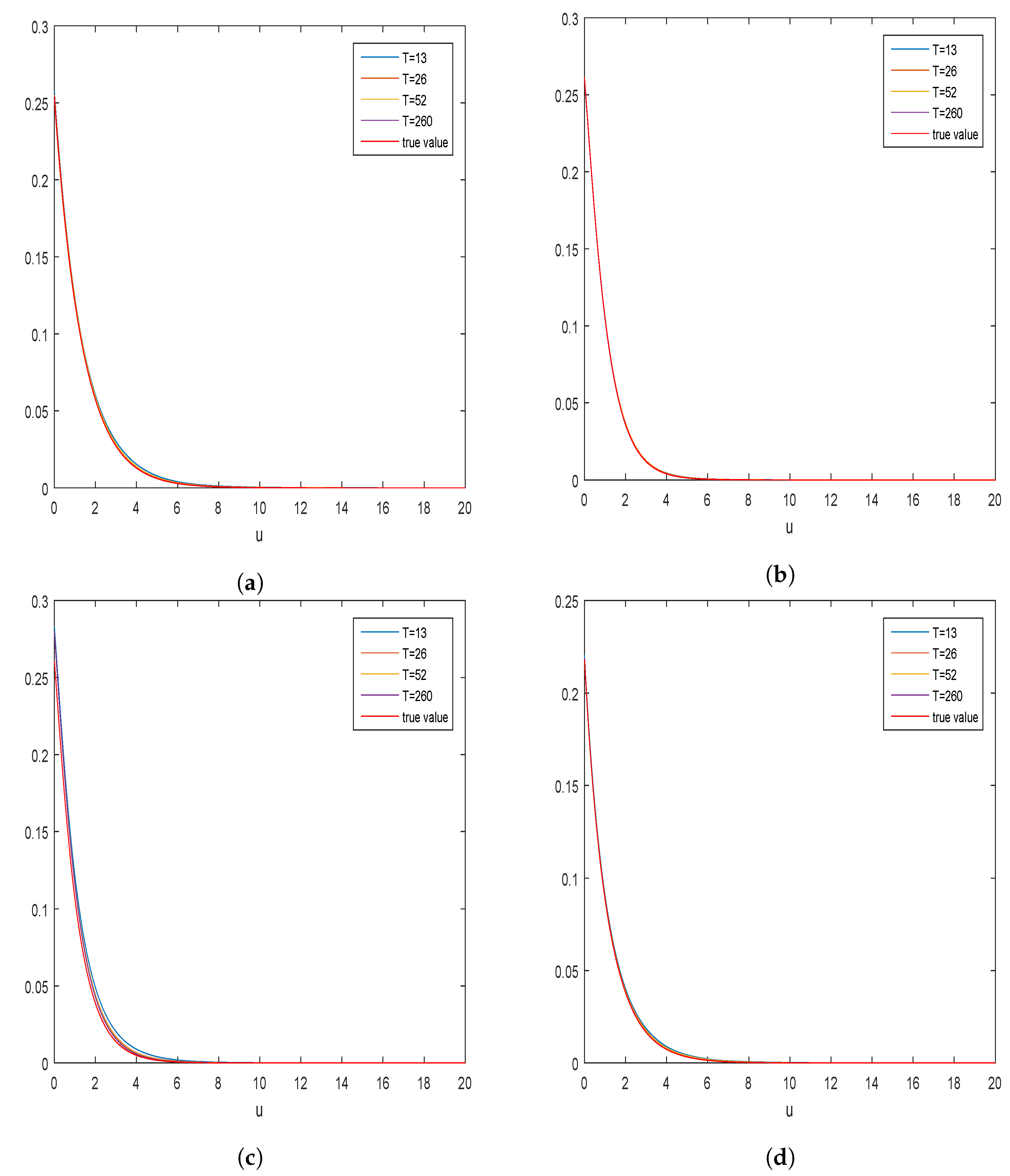
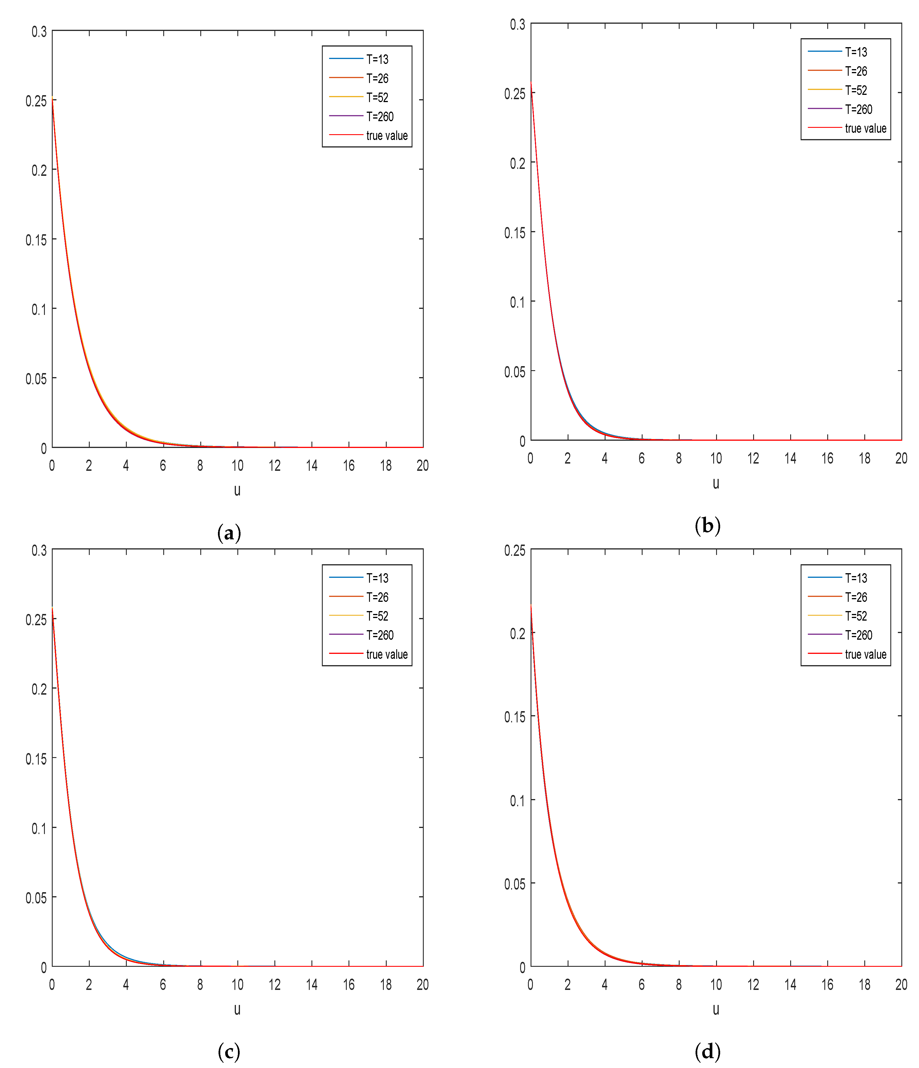
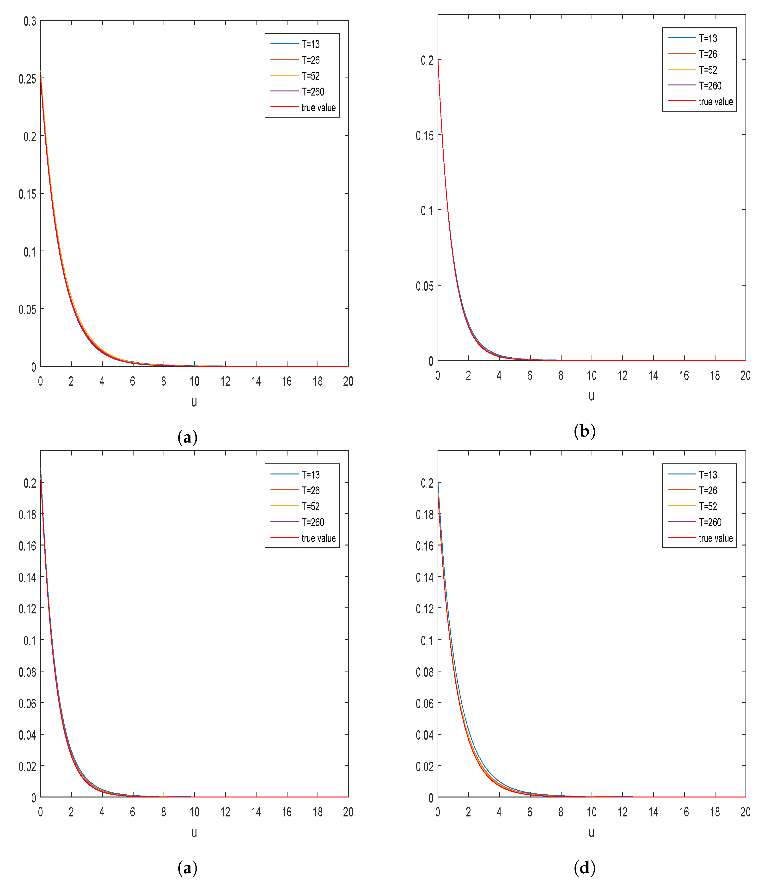
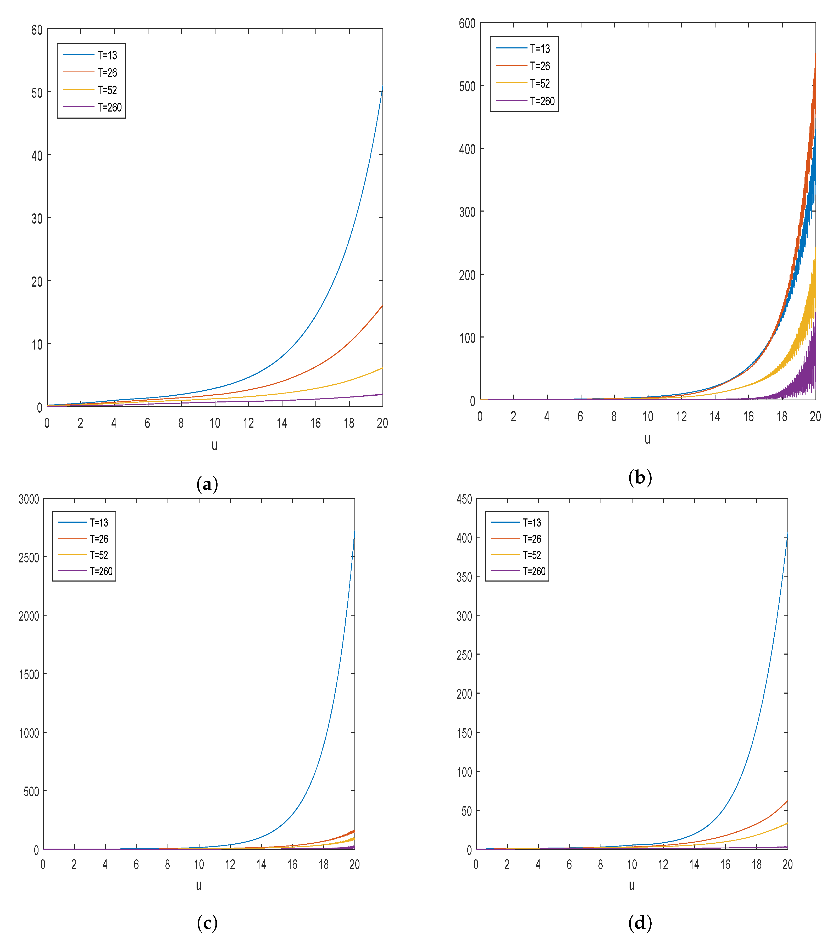
5. Simulation Studies

In this section, we present some numerical examples to explain the excellent properties of our estimator when the observed sample is finite. We mainly studied the following three kinds of special expected discounted penalty function:

(1) Ruin probability (RP: $\mathrm{w}\equiv 1,\delta =0)$;

(2) Laplace transform of ruin time (LT: $\mathrm{w}\equiv 1,\delta =0.1)$;

(3) Expected discounted deficit at ruin (EDD) when ruin is due to a claim $\left(\mathrm{w}\right(x,y)=y,\delta =0.1)$.

Some simulation examples of the above functions are presented for different distributions of claim sizes:

(1) Exponential distribution: $f\left(x\right)=e^{-x},x>0$;

(2) Erlang(2) distribution: $f\left(x\right)=4x{e}^{-2x},x>0$;

(3) Combined exponential distribution: $f\left(x\right)=3e^{-1.5x}-3e^{-3x},x>0$;

(4) Mixed exponential distribution: $f\left(x\right)=\frac{2}{3}{e}^{-2x}+\frac{2}{3}{e}^{-x},x>0$.

We set $\Delta =1,\lambda =2$, and $\mu =5$, where $\Delta =1$ can be explained as one week. That is to say, in a long time interval, the insurer will observe the data once a week, the expected claim number is 2 times per week, and the expected premium number is 5 times per week. Furthermore, since there are 52 business weeks every year, we assumed that ${\displaystyle T=\frac{1}{4}\times 52\times \Delta ,T=\frac{1}{2}\times 52\times \Delta ,T=1\times 52\times \Delta ,T=5\times 52\times \Delta }$, which means that we observed the surplus process for one quarter, half a year, one year and five years. Then, we used Equation (13) to estimate the above Gerber-Shiu functions, and the corresponding true value obtained by Laplace inversion. In all simulations, we set $c=5,a=30,K=2^{13}$, and we carried out the relevant analysis based on 300 simulation experiments. We first introduce several concepts used in this section. The mean value and the mean relative error, which are, respectively, defined by

$$\frac{1}{300}\sum _{j=1}^{300}{\widehat{\Phi }}_{K,a,j}\left(u\right),\frac{1}{300}\sum _{j=1}^{300}\left|\frac{{\widehat{\Phi }}_{K,a,j}\left(u\right)}{\Phi \left(u\right)}-1\right|,$$

and the integrated mean square error (IMSE), which is defined by

$$\frac{1}{300}\sum _{j=1}^{300}{\int }_0^{\infty }{({\widehat{\Phi }}_{K,a,j}\left(u\right)-\Phi \left(u\right))}^{2}du\approx \frac{1}{300}\sum _{j=1}^{300}{\int }_0^{30}{({\widehat{\Phi }}_{K,a,j}\left(u\right)-\Phi \left(u\right))}^{2}du,$$

where ${\widehat{\Phi }}_{K,a,j}\left(u\right)$ is the estimate of expected discounted penalty function in the jth experiment. For IMSE, we computed the integral on the finite domain $[0,30]$, as both the true value and the estimator will be very small when $u\ge 30$. In reality, both the true value and the estimated value are very close to zero when $u>20$, thus we present all images for $u\in [0,20]$ to illustrate the performance of our estimators better.

First, we plot the mean curves of the estimated expected discounted penalty functions and compare them with the corresponding true curves. For the above-mentioned four distributions of claim sizes, we show the mean curves and the true curves of RP, LT, EDD due to a claim in Figure 1, Figure 2 and Figure 3, respectively. It is easily observed that, even though we used the quarter book data, the performance of the estimation for each claim distribution was still good. We could hardly distinguish the true curves from the mean curves when we used the five-year book data. Since it is difficult to distinguish the mean curves for different T values when u becomes large, we further show the mean relative error curves of the estimated expected discounted penalty functions for different claim distributions in Figure 4, Figure 5 and Figure 6, respectively. We observed that the mean relative errors became small as T increased, and they were very small when $T=260$. Besides, we found that the mean relative errors were small when u was small, but became very large when u was large. This is because the true values of the expected discounted penalty functions were very small when u was large. All of the above results illustrate the performance of our estimations by images. Finally, we present some values of IMSE for the estimators of RP, LT, and EDD in

Table 1. IMSE of ${\widehat{\Phi }}_{K,a}$.

T	Exp			Erlang(2)
	RP	LT	EDD	RP	LT	EDD
13	0.00717	0.00644	0.01586	0.00351	0.00414	0.00412
26	0.00352	0.00316	0.00846	0.00186	0.00200	0.00214
52	0.00177	0.00199	0.00537	0.00108	0.00099	0.00095
260	0.00032	0.00034	0.00092	0.00018	0.00020	0.00019

and

Table 2. IMSE of ${\widehat{\Phi }}_{K,a}$.

T	Com-Exp			Mix-Exp
	RP	LT	EDD	RP	LT	EDD
13	0.00719	0.00431	0.00527	0.00474	0.00511	0.01176
26	0.00271	0.00195	0.00277	0.00267	0.00233	0.00602
52	0.00160	0.00114	0.00124	0.00117	0.00107	0.00257
260	0.00046	0.00021	0.00024	0.00025	0.00018	0.00053

to further show that our estimators perform well. Combining all of the simulation results, we conclude that our estimators could effectively approximate the true values, and they performed well for the large T.

References

1. Gerber, H.U.; Shiu, E.S.W. On the time value of ruin. N. Am. Actuar. J. 1998, 2, 48–78. [Google Scholar] [CrossRef]
2. Lin, X.S.; Willmot, G.E.; Drekic, S. The classical risk model with a constant dividend barrier: Analysis of the Gerber-Shiu discounted penalty function. Insur. Math. Econ. 2003, 33, 391–408. [Google Scholar]
3. Yuen, K.C.; Wang, G.J.; Li, W.K. The Gerber-Shiu expected discounted penalty function for risk processes with interest and a constant dividend barrier. Insur. Math. Econ. 2007, 40, 104–112. [Google Scholar] [CrossRef]
4. Yuen, K.C.; Zhou, M.; Guo, J.Y. On a risk model with debit interest and dividend payments. Stat. Probab. Lett. 2008, 78, 2426–2432. [Google Scholar] [CrossRef]
5. Zhao, X.H.; Yin, C.C. The Gerber-Shiu expected discounted penalty function for Lévy insurance risk processes. Acta Math. Sin. 2010, 26, 575–586. [Google Scholar] [CrossRef]
6. Chi, Y.C. Analysis of expected discounted penalty function for a general jump diffusion risk model and applications in finance. Insur. Math. Econ. 2010, 46, 385–396. [Google Scholar] [CrossRef]
7. Yin, C.C.; Wang, C.W. The perturbed compound Poisson risk process with investment and debit Interest. Methodol. Comput. Appl. 2010, 12, 391–413. [Google Scholar] [CrossRef]
8. Chi, Y.C.; Lin, X.S. On the threshold dividend strategy for a generalized jump-diffusion risk model. Insur. Math. Econ. 2011, 48, 326–337. [Google Scholar] [CrossRef]
9. Shen, Y.; Yin, C.C.; Yuen, K.C. Alternative approach to the optimality of the threshold strategy for spectrally negative Lévy processes. Acta Math. Appl. Sin. Engl. 2013, 29, 705–716. [Google Scholar] [CrossRef]
10. Yin, C.C.; Yuen, K.C. Exact joint laws associated with spectrally negative Lévy processes and applications to insurance risk theory. Front. Math. China 2014, 9, 1453–1471. [Google Scholar] [CrossRef]
11. Zhao, Y.X.; Yao, D.J. Optimal dividend and capital injection problem with a random time horizon and a ruin penalty in the dual model. Appl. Math. Ser. B 2015, 30, 325–339. [Google Scholar] [CrossRef]
12. Li, S.M.; Lu, Y.; Sendova, K.P. The expected discounted penalty function: From infinite time to finite time. Scand. Actuar. J. 2019. [Google Scholar] [CrossRef]
13. Li, Y.Q.; Yin, C.C.; Zhou, X.W. On the last exit times for spectrally negative Lévy processes. J. Appl. Probab. 2017, 54, 474–489. [Google Scholar] [CrossRef] [Green Version]
14. Dong, H.; Yin, C.C.; Dai, H.S. Spectrally negative Lévy risk model under Erlangized barrier strategy. J. Comput. Appl. Math. 2019, 351, 101–116. [Google Scholar] [CrossRef]
15. Wang, W.Y.; Zhang, Z.M. Computing the Gerber-Shiu function by frame duality projection. Scand. Actuar. J. 2019. [Google Scholar] [CrossRef]
16. Willmot, G.E.; Dickson, D.C.M. The Gerber-Shiu discounted penalty function in the stationary renewal risk model. Insur. Math. Econ. 2003, 32, 403–411. [Google Scholar] [CrossRef]
17. Wang, C.W.; Yin, C.C.; Li, E.Q. On the classical risk model with credit and debit interests under absolute ruin. Stat. Probab. Lett. 2010, 80, 427–436. [Google Scholar] [CrossRef]
18. Yin, C.C.; Yuen, K.C. Optimality of the threshold dividend strategy for the compound Poisson model. Stat. Probab. Lett. 2011, 81, 1841–1846. [Google Scholar] [CrossRef]
19. Dong, H.; Yin, C.C. Complete monotonicity of the probability of ruin and DE Finetti’s dividend problem. J. Syst. Sci. Complex. 2012, 25, 178–185. [Google Scholar] [CrossRef]
20. Yu, W.G. Some results on absolute ruin in the perturbed insurance risk model with investment and debit interests. Econ. Model. 2013, 31, 625–634. [Google Scholar] [CrossRef]
21. Yin, C.C.; Shen, Y.; Wen, Y.Z. Exit problems for jump processes with applications to dividend problems. J. Comput. Appl. Math. 2013, 245, 30–52. [Google Scholar] [CrossRef]
22. Zeng, Y.; Li, D.P.; Gu, A.L. Robust equilibrium reinsurance-investment strategy for a mean-variance insurer in a model with jumps. Insur. Math. Econ. 2016, 66, 138–152. [Google Scholar] [CrossRef]
23. Zhao, Y.X.; Wang, R.M.; Yao, D.J. Optimal dividend and equity issuance in the perturbed dual model under a penalty for ruin. Commun. Stat. Theory Methods 2016, 45, 365–384. [Google Scholar] [CrossRef]
24. Yu, W.G.; Huang, Y.J.; Cui, C.R. The absolute ruin insurance risk model with a threshold dividend strategy. Symmetry 2018, 10, 377. [Google Scholar] [CrossRef]
25. Boucherie, R.J.; Boxma, O.J.; Sigman, K. A note on negative customers, GI/G/1 workload, and risk process. Probab. Eng. Inf. Sci. 1997, 11, 305–311. [Google Scholar] [CrossRef]
26. Boikov, A.V. The Cramér-Lundberg model with stochastic premium process. Theory Probab. Appl. 2003, 47, 489–493. [Google Scholar] [CrossRef]
27. Temnov, G. Risk process with random income. J. Math. Sci. 2004, 123, 3780–3794. [Google Scholar] [CrossRef]
28. Bao, Z.H. The expected discounted penalty at ruin in the risk process with random income. Appl. Math. Comput. 2006, 179, 559–566. [Google Scholar] [CrossRef]
29. Bao, Z.H.; Ye, Z.X. The Gerber-Shiu discounted penalty function in the delayed renewal risk process with random income. Appl. Math. Comput. 2007, 184, 857–863. [Google Scholar] [CrossRef]
30. Yang, H.; Zhang, Z.M. On a class of renewal risk model with random income. Appl. Stoch. Model. Bus. 2009, 25, 678–695. [Google Scholar] [CrossRef]
31. Labbé, C.; Sendova, K.P. The expected discounted penalty function under a risk model with sochastic income. Appl. Math. Comput. 2009, 215, 1852–1867. [Google Scholar]
32. Zhang, Z.M.; Yang, H. On a risk model with stochastic premiums income and dependence between income and loss. J. Comput. Appl. Math. 2010, 234, 44–57. [Google Scholar] [CrossRef] [Green Version]
33. Zhao, Y.X.; Yin, C.C. The expected discounted penalty function under a renewal risk model with stochastic income. Appl. Math. Comput. 2012, 218, 6144–6154. [Google Scholar] [CrossRef]
34. Xu, L.; Wang, R.M.; Yao, D.J. On maximizing the expected terminal utility by investment and reinsurance. J. Ind. Manag. Optim. 2008, 4, 801–815. [Google Scholar]
35. Yu, W.G. On the expected discounted penalty function for a Markov regime switching risk model with stochastic premium income. Discret. Dyn. Nat. Soc. 2013, 2013, 1–9. [Google Scholar] [CrossRef]
36. Yu, W.G. Randomized dividends in a discrete insurance risk model with stochastic premium income. Math. Probl. Eng. 2013, 2013, 1–9. [Google Scholar] [CrossRef]
37. Zhou, J.M.; Mo, X.Y.; Ou, H.; Yang, X.Q. Expected present value of total dividends in the compound binomial model with delayed claims and random income. Acta Math. Sci. 2013, 33, 1639–1651. [Google Scholar] [CrossRef]
38. Gao, J.W.; Wu, L.Y. On the Gerber-Shiu discounted penalty function in a risk model with two types of delayed-claims and random income. J. Comput. Appl. Math. 2014, 269, 42–52. [Google Scholar] [CrossRef]
39. Zhou, M.; Yuen, K.C.; Yin, C.C. Optimal investment and premium control in a nonlinear diffusion model. Acta Math. Appl. Sin. Engl. 2017, 33, 945–958. [Google Scholar] [CrossRef]
40. Deng, Y.C.; Liu, J.; Huang, Y.; Li, M.; Zhou, J.M. On a discrete interaction risk model with delayed claims and stochastic incomes under random discount rates. Commun. Stat. Theory Methods 2018, 47, 5867–5883. [Google Scholar] [CrossRef]
41. Zeng, Y.; Li, D.P.; Chen, Z.; Yang, Z. Ambiguity aversion and optimal derivative-based pension investment with stochastic income and volatility. J. Econ. Dyn. Control 2018, 88, 70–103. [Google Scholar] [CrossRef]
42. Politis, K. Semiparametric estimation for non-ruin probabilities. Scand. Actuar. J. 2003, 2003, 75–96. [Google Scholar] [CrossRef]
43. Wang, Y.F.; Yin, C.C. Approximation for the ruin probabilities in a discrete time risk model with dependent risks. Stat. Probab. Lett. 2010, 80, 1335–1342. [Google Scholar] [CrossRef]
44. Yuen, K.C.; Yin, C.C. Asymptotic results for tail probabilities of sums of dependent and heavy-tailed random variables. Chin. Ann. Math. B 2012, 33, 557–568. [Google Scholar] [CrossRef]
45. Zhang, Z.M.; Yang, H.L.; Yang, H. On a nonparametric estimator for ruin probability in the classical risk model. Scand. Actuar. J. 2014, 2014, 309–338. [Google Scholar] [CrossRef]
46. Wang, Y.F.; Yin, C.C.; Zhang, X.S. Uniform estimate for the tail probabilities of randomly weighted sums. Acta Math. Appl. Sin. Engl. 2014, 30, 1063–1072. [Google Scholar] [CrossRef]
47. Zhang, Z.M. Nonparametric estimation of the finite time ruin probability in the classical risk model. Scand. Actuar. J. 2017, 2017, 452–469. [Google Scholar] [CrossRef]
48. Zhang, Z.M.; Yang, H.L. Nonparametric estimate of the ruin probability in a pure-jump Lévy risk model. Insur. Math. Econ. 2013, 53, 24–35. [Google Scholar] [CrossRef] [Green Version]
49. Zhang, Z.M.; Yang, H.L. Nonparametric estimation for the ruin probability in a Lévy risk model under low-frequency observation. Insur. Math. Econ. 2014, 59, 168–177. [Google Scholar] [CrossRef] [Green Version]
50. Shimizu, Y.; Zhang, Z.M. Estimating Gerber-Shiu functions from discretely observed Lévy driven surplus. Insur. Math. Econ. 2017, 74, 84–98. [Google Scholar] [CrossRef]
51. Peng, J.Y.; Wang, D.C. Asymptotics for ruin probabilities of a non-standard renewal risk model with dependence structures and exponential lévy process investment returns. J. Ind. Manag. Optim. 2017, 13, 155–185. [Google Scholar] [CrossRef]
52. Peng, J.Y.; Wang, D.C. Uniform asymptotics for ruin probabilities in a dependent renewal risk model with stochastic return on investments. Stochastics 2018, 90, 432–471. [Google Scholar] [CrossRef]
53. Yang, Y.; Wang, K.Y.; Liu, J.J.; Zhang, Z.M. Asymptotics for a bidimensional risk model with two geometric Lévy price processes. J. Ind. Manag. Optim. 2019, 15, 481–505. [Google Scholar] [CrossRef]
54. Yang, Y.; Yuen, K.C.; Liu, J.F. Asymptotics for ruin probabilities in Lévy-driven risk models with heavy-tailed claims. J. Ind. Manag. Optim. 2018, 14, 231–247. [Google Scholar] [CrossRef]
55. Shimizu, Y. Estimation of the expected discounted penalty function for Lévy insurance risks. Math. Methods Stat. 2011, 20, 125–149. [Google Scholar] [CrossRef]
56. Zhang, Z.M. Estimating the Gerber-Shiu function by Fourier-Sinc series expansion. Scand. Actuar. J. 2017, 2017, 898–919. [Google Scholar] [CrossRef]
57. Zhang, Z.M.; Su, W. A new efficient method for estimating the Gerber-Shiu function in the classical risk model. Scand. Actuar. J. 2018, 2018, 426–449. [Google Scholar] [CrossRef]
58. Zhang, Z.M.; Su, W. Estimating the Gerber-Shiu function in a Lévy risk model by Laguerre series expansion. J. Comput. Appl. Math. 2019, 346, 133–149. [Google Scholar] [CrossRef]
59. Su, W.; Yong, Y.D.; Zhang, Z.M. Estimating the Gerber-Shiu function in the perturbed compound Poisson model by Laguerre series expansion. J. Math. Anal. Appl. 2019, 469, 705–729. [Google Scholar] [CrossRef]
60. Fang, F.; Oosterlee, C.W. A novel option pricing method based on Fourier cosine series expansions. SIAM J. Sci. Comput. 2008, 31, 826–848. [Google Scholar] [CrossRef]
61. Fang, F.; Oosterlee, C.W. Pricing early-exercise and discrete barrier options by Fourier-cosine series expansions. Numer. Math. 2009, 114, 27–62. [Google Scholar] [CrossRef]
62. Zhang, B.; Oosterlee, C.W. Pricing of early-exercise Asian options under Lévy processes based on Fourier cosine expansions. Appl. Numer. Math. 2014, 78, 14–30. [Google Scholar] [CrossRef] [Green Version]
63. Chau, K.W.; Yam, S.C.P.; Yang, H.L. Fourier-cosine method for Gerber-Shiu functions. Insur. Math. Econ. 2015, 61, 170–180. [Google Scholar] [CrossRef]
64. Chau, K.W.; Yam, S.C.P.; Yang, H.L. Fourier-cosine method for ruin probabilities. J. Comput. Appl. Math. 2015, 281, 94–106. [Google Scholar] [CrossRef] [Green Version]
65. Zhang, Z.M. Approximating the density of the time to ruin via Fourier-cosine series expansion. Astin Bull. 2017, 47, 169–198. [Google Scholar] [CrossRef]
66. Yang, Y.; Su, W.; Zhang, Z.M. Estimating the discounted density of the deficit at ruin by Fourier cosine series expansion. Stat. Probab. Lett. 2019, 146, 147–155. [Google Scholar] [CrossRef]
67. Dickson, D.C.M.; Hipp, C. On the time to ruin for Erlang(2) risk processes. Insur. Math. Econ. 2001, 29, 333–344. [Google Scholar] [CrossRef]
68. Li, S.M.; Garrido, J. On ruin for the Erlang(n) risk process. Insur. Math. Econ. 2004, 34, 391–408. [Google Scholar] [CrossRef]
69. Van Der Vaart, A.W. Asymptotic Statistics; Cambridge University Press: Cambridge, UK, 1998. [Google Scholar]
Figure 1. Estimation of the ruin probability for different claim sizes. Mean curves: (a) exponential claim sizes; (b) Erlang claim sizes; (c) combined-exponential claim sizes; and (d) mixed-exponential claim sizes.
Mathematics 07 00305 g001
Figure 2. Estimation of the Laplace transform of ruin time for different claim sizes. Mean curves: (a) exponential claim sizes; (b) Erlang claim sizes; (c) combined-exponential claim sizes; and (d) mixed-exponential claim sizes.
Mathematics 07 00305 g002
Figure 3. Estimation of the expected discounted deficit at ruin due to a claim for different claim sizes. Mean curves: (a) exponential claim sizes; (b) Erlang claim sizes; (c) combined-exponential claim sizes; and (d) mixed-exponential claim sizes.
Mathematics 07 00305 g003
Figure 4. Estimation of the ruin probability for different claim sizes. Mean relative error curves: (a) exponential claim sizes; (b) Erlang claim sizes; (c) combined-exponential claim sizes; and (d) mixed-exponential claim sizes.
Mathematics 07 00305 g004
Figure 5. Estimation of the Laplace transform of ruin time for different claim sizes. Mean relative error curves: (a) exponential claim sizes; (b) Erlang claim sizes; (c) combined-exponential claim sizes; and (d) mixed-exponential claim sizes.
Mathematics 07 00305 g005aMathematics 07 00305 g005b
Figure 6. Estimation of the expected discounted deficit at ruin due to a claim for different claim sizes. Mean relative error curves: (a) exponential claim sizes; (b) Erlang claim sizes; (c) combined-exponential claim sizes; and (d) mixed-exponential claim sizes.
Mathematics 07 00305 g006