Abstract
Topological indices are numerical values associated with a graph (structure) that can predict many physical, chemical, and pharmacological properties of organic molecules and chemical compounds. The distance degree () index was introduced by Dobrynin and Kochetova in 1994 for characterizing alkanes by an integer. In this paper, we have determined expressions for a index of some derived graphs in terms of the parameters of the parent graph. Specifically, we establish expressions for the index of a line graph, subdivision graph, vertex-semitotal graph, edge-semitotal graph, total graph, and paraline graph.
MSC:
05C10; 05C12; 05C76
1. Introduction
Graph theory is becoming interestingly significant as it is being actively applied in biochemistry, nanotechnology, electrical engineering, computer science, and operations research [1,2,3,4]. The powerful combinatorial method found in graph theory has also been used to prove the results of pure mathematics. A topological index, also known as a graph descriptor, is a real number associated with a graph. Topological indices are helpful for predicting certain physical, chemical, and pharmacological properties of organic molecules and chemical compounds.
A molecular graph is a graphical description of the structural formula of a chemical compound with the help of graph theory. In the construction of a chemical graph, atoms are represented by nodes or vertices and bonds between the atoms are represented by lines or edges [5]. In all major fields of chemistry, chemical graphs are used for many different purposes [6]. As has already been proved in [7], the said indices are useful for characterizing alkanes by an integer. Although the computed expression does not have direct application, we believe that it can be used to compute the said indices for chemical and molecular graphs, which are useful for characterizing alkanes by an integer.
All graphs considered in this paper are simple and connected. Let be a simple and connected graph with vertex set and edge set . The degree of vertex in is denoted by and is defined as the number of edges incident with vertex . Also, the degree of an edge in is denoted by and is defined as the number of edges incident to both its end vertices, and . Mathematically, . A complete graph on vertices is denoted by and defined as a graph in which every vertex is adjacent to all other vertices. Let and be two subgraphs of , such that . Let and be the vertices such that
then and are called the terminal vertices of subgraphs and in , as shown in the following figure.
In Figure 1, and are subgraphs of graph . In graph , the distance between vertex of and the vertex of is 1, which is the minimum of all vertices of and . So, and are known as terminal vertices of and in .
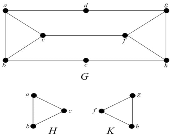
Figure 1.
Graph with its subgraphs and .
The first and second Zagreb indices were defined by Gutman and Trinajastić in 1972 [8] and very useful in QSPR and QSAR [9,10,11]. The first and second Zagreb index are defined as:
and
Another vertex-degree based topological index was found to be useful in the earliest work on Zagreb indices [8], but later it was totally ignored. Quite recently, some interest was shown in it [12,13]. It is called the Forgotten index or simply F-index and defined as:
In 2008, Došlić introduced the first Zagreb coindex [14], which is defined as:
In 1947, the chemist Harold Wiener introduced the Wiener index [15], which correlates to the boiling point and structure of the molecule of paraffins. The Wiener index is the oldest topological index and is defined as:
where is the distance in between the vertices and . The Wiener index attracts many chemists and mathematicians and has a long history in the literature. For details, see [16,17,18,19,20,21]. For the applications of the molecular structures, see [22].
The edge version of the Wiener index was introduced in 2010 [23], and is defined as:
where is the distance between the edges and in and defined as:
The degree distance index ( index) was introduced in [7] by Dobrynin and Kochetova and is defined as:
For a brief look at the different results of index, see [24,25,26,27,28,29]. We define an edge version of index as,
The distance between the edge and a vertex is defined as
For basic terminology, see [30].
1.1. Some Derived Graphs
- Line Graph: Line graph of a graph is denoted by such that and there is an edge between two vertices of if and only if corresponding edges are incident in . Clearly, and by hand shaking-lemma one can easily see that .
- Subdivision Graph: Subdivision graph of a graph is obtained by inserting a vertex of degree in each edge. Therefore, and .
- Vertex-Semitotal Graph: Vertex-Semitotal graph of a graph is denoted as and is obtained by adding a new vertex to each edge of and then joining a new vertex to the end vertices of the corresponding edge. Thus, and
- Edge-Semitotal Graph: The edge-semitotal graph of a graph is denoted as and is obtained by inserting a new vertex ateach edge of , joining those new vertices by edges whose corresponding edges are incident in . We have and
- Total Graph: The union of edge-semitotal graph and vertex-semitotal graph is called total graph of a graph . It is denoted by . Also,
- Paraline Graph: The paraline graph is the line graph of subdivision graph denoted by . Also and
In [20], one sees that . Thus,
In Figure 2, self-explanatory examples of these derived graphs are given for a particular graph. In every derived graph of (except the paraline graph ), the vertices corresponding to the vertices of are denoted by circles and the vertices corresponding to the edges of are denoted by squares.
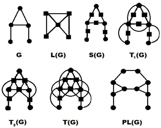
Figure 2.
Different graphs derived from .
The following is a known result of Zagreb indices.
Lemma 1.
[31] For a graph with vertices and edges, we have
1.2. Index of Some Derived Graphs
In [31,32,33] the authors studied the expressions for Zagreb indices and multiplicative Zagreb indices of aforementioned derived graphs. In the past authors dealt only with degree-based indices to derive expressions for the derived graphs. The following proposition encourages us to deal with degree distance-based index. In this section, we study degree distance-based index, index for these derived graphs.
Proposition 1.
Ifis line graph of a graph, then
For a subdivision graph , a vertex-semitotal graph , an edge-semitotal graph , and a total graph , we can categorize the vertex set into two types of vertices. The first is the set of vertices of and the second is the set of vertices corresponding to the edges of . We name them -type and -type vertices, respectively. On the basis of this division, there are three types of edges in these graphs:
- -edge, an edge between two -type vertices,
- -edge, an edge between two -type vertices,
- -edge, an edge between an -type vertex and a -type vertex.
Theorem 1.
Ifis a subdivision graph of graph, then
Proof.
We can see that for any -type vertex of
and for any type vertex of
Also,
By definition of the index, we have
□
Theorem 2.
Ifis the vertex-semitotal graph of graph, then
Proof.
First note that for any -type vertex of
and for any -type vertex of
We have
Since
Therefore,
□
Theorem 3.
Ifis an edge-semitotal graph of graph, then
Proof.
To prove this theorem, we proceed in a similar way.
First note that for any -type vertex of
and for any -type vertex of
So,
Using the Lemma 1 and relation
So,
□
Theorem 4.
Ifis the total graph of graph, then
Proof.
First note that for any -type vertex of
and for any -type vertex of
Also,
□
Lemma 2.
For graphthe following equality holds.
Proof.
First we calculate
Now the above calculated expression can be written as follows:
which gives us the equation
which completes the proof. □
Theorem 5.
Letbe a graph having no cycle of even length. Ifis a paraline graph of, then
Proof.
It can be noted that for any vertex there are vertices in having the same degree as the vertex such that all the vertices are connected with each other. In fact, can be obtained from by replacing every vertex by .
By definition of the index,
Now, either or belongs to the same or two different values, where . So,
Here we discuss the two terms one by one.
- In the first term, for any vertex there are a total of pairs of vertices in of degrees and having a distance of 1 between them in the corresponding .
- Before discussing the second term, it is important to see that there is exactly one shortest path in between any two different vertices, because has no cycle of even length. Consequently, there is exactly one shortest path between their corresponding complete graphs in .
Now, in the second term, for any pair of vertices and in , we have the following cases in corresponding pair of complete graphs and in :
- Case-1:
- There is exactly one pair of terminal vertices in and , having distance between them.
- Case-2:
- There are pairs of non-terminal vertices in and , having distance between them.
- Case-3:
- There are pairs of vertices having a non-terminal vertex in and a terminal vertex in , and having distance between them. Similarly, there are pairs of vertices having a terminal vertex in and a non-terminal vertex in , and having distance between them. So we have a total of such pairs.
Thus, in light of the above discussion, we have
By using Lemma 2, we have
□
2. Conclusions
In this paper, we studied the index of derived graphs, which involves distance and degrees. We computed the expressions to find the index of the derived graph by using the parent graph. More specifically, we found the expressions of the index using some topological indices of the parent graph. As has already been proved, the said indices are useful for characterizing alkanes by an integer. Although the computed expression does not have direct application, we believe that it can be used to compute the said indices for chemical and molecular graphs, which are useful for characterizing alkanes by an integer.
Author Contributions
These authors contributed equally to this work.
Funding
This work was supported by the Teaching Groups in Anhui Province (2016jytd080, 2015jytd048); the Natural Science Foundation of the Education Department of Anhui Province (KJ2017A704), the Key Program of the Excellent Young Talents Support of Higher Education in Anhui Province (gxyq2018116); the Natural Science Foundation of Bozhou University (BYZ2018B03).
Acknowledgments
Authors are thankful to the referees for their valuable comments to improve this paper.
Conflicts of Interest
The authors declare no conflict of interest.
References
- Tadic, B.; Ziukovic, J. The graph theory frame work for odeling nano scale systems. Nanoscale Syst. MMTA 2013, 2, 30–48. [Google Scholar]
- Balaban, A.T. Applications of graph theory in chemistry. J. Chem. Inf. Comput. Sci 1985, 25, 334–343. [Google Scholar] [CrossRef]
- Abdullahi, S. Anapplication of graph theory to the electrical circuit using matrix method. J. Math. 2014, 164–166. [Google Scholar] [CrossRef]
- Shirinivas, S.G.; Vetrivel, S.; Elango, N.M. Applications of graph theory in computer science an overview. J. Eng. Technol. 2010, 2, 4610–4621. [Google Scholar]
- Gold, V.; Loening, K.L.; McNaught, A.D.; Shemi, P. Compendium of Chemical Terminology; Blackwell Science Oxford: Oxford, UK, 1997; Volume 1669. [Google Scholar]
- Bonchev, D.; Rouvray, D.H. Chemical Graph Theory Introductions and Fundamentals; CRC Press: Boca Raton, FL, USA, 1991; Volume 1. [Google Scholar]
- Dobrynin, A.A.; Kochetova, A.A. Degree distance of a graph: A degree analogue of the Wiener index. J. Chem. Inf. Comput. Sci. 1994, 34, 1082–1086. [Google Scholar] [CrossRef]
- Gutman, I.; Trinajstić, N. Graph theory and molecular orbitals III. Total Electron Energy Altern. Hydrocarb. Chem. Phys. Lett. 1972, 17, 535–538. [Google Scholar]
- Balaban, A.T. From Chemical Topology to Three-Dimensional Geometry; Plenum Press: New York, NY, USA, 1997. [Google Scholar]
- Devillers, J.; Balaban, A.T. (Eds.) Topological Indices and Related Descriptors in QSAR and QSPR; Gordon and Breach: Amsterdam, The Netherlands, 1999. [Google Scholar]
- Todeschini, R.; Consonni, V. Handbook of Molecular Descriptors; Wiley–VCH: Weinheim, Germany, 2000. [Google Scholar]
- Furtula, B.; Gutman, I. A forgotten topological index. J. Math. Chem. 2015, 53, 1184–1190. [Google Scholar] [CrossRef]
- De, N.; Nayeem, S.M.A.; Pal, A. The F-coindex of some graph operations. Springer Plus 2016, 5, 221. [Google Scholar] [CrossRef] [PubMed]
- Došlic, T. Vertex-weighted Wiener polynomials for composite graphs. Ars Math. Contemp. 2008, 1, 66–80. [Google Scholar] [CrossRef]
- Wiener, H. Structural determination of Paraffin boiling points. J. Am. Chem. Soc. 1947, 69, 17–20. [Google Scholar] [CrossRef]
- Ashrafi, A.R.; Yousafi, S. An exact expression for the Wiener index of a polyhex nanotorus. MATCH Commun. Math. Comput. Chem. 2006, 56, 169–178. [Google Scholar]
- Ashrafi, A.R.; Yousafi, S. A new algorithm for computing distance matrix and Wiener index of zig-zag polyhex nano-tubes, nano-scale. Res. Lett. 2007, 2, 202–206. [Google Scholar]
- Chepoi, V.; Kalvzar, S. The Wiener index and the Szeged index of benzoid systems in linear time. J. Chem. Inf. Comput. Sci. 1997, 37, 752–755. [Google Scholar] [CrossRef]
- Cai, X.; Zhou, B. Reverse Wiener index of connected graphs, MATCH Commun. Math. Comput. Chem. 2008, 60, 95–105. [Google Scholar]
- Dobrynin, A.A.; Entringer, R.; Gutman, I. Wiener index of trees, Theory and applications. Acta App. Math. 2011, 66, 211–249. [Google Scholar] [CrossRef]
- Dobrynin, A.A.; Gutman, I.; Klavzar, S.; Zigerl, P. Wiener index of hexagonal systems. Accta. Appl. Math. 2001, 72, 247–294. [Google Scholar] [CrossRef]
- Sandberg, T.O.; Weinberger, C.; Smått, J.H. Molecular dynamics on wood-derived lignans analyzed by intermolecular network theory. Molecules 2018, 23, 1990. [Google Scholar] [CrossRef] [PubMed]
- Iranmanesh, A.; Gutman, I.; Khormali, O.; Mahmiani, A. The edge versions of Wiener index. Match Commun. Math. Comput. Chem. 2009, 61, 663–672. [Google Scholar]
- Ali, P.; Mukwembi, S.; Munyria, S. Degree distance and vertex connectivity. Disc. Appl. Math. 2013, 161, 2802–2811. [Google Scholar] [CrossRef]
- Du, Z.; Zhou, B. Degree distance of a graph. Filomat 2010, 24, 95–120. [Google Scholar] [CrossRef]
- Ilic, A.; Stevanovic, D.; Feng, L.; Yu, G.; Danklemann, P. Degree distance of unicyclic graphs. Discr. Appl. Math. 2011, 159, 779–788. [Google Scholar] [CrossRef]
- Tomescu, I. Unicyclic and bicyclic graphs having minmum degree distance. Discr. Appl. Math. 2008, 156, 125–130. [Google Scholar] [CrossRef]
- Tomescu, I. Properties of connected graphs having minimum degree distance. Discr. Appl. Math. 2008, 309, 2745–2748. [Google Scholar] [CrossRef]
- Tomsecu, I. Ordering connected graphs having small degree distance. Discr. Appl. Math. 2010, 158, 1714–1717. [Google Scholar] [CrossRef]
- Bondy, J.A.; Murty, U.S.R. Graph Theory; Springer: Berlin, Germany, 2008. [Google Scholar]
- Gutman, I.; Furtula, B.; Kovijanic, Z.; Vukicevic; Popivoda, G. On Zagreb indices and coindices. Match Commun. Math. Comput. Chem. 2015, 74, 5–16. [Google Scholar]
- Basavanagoud, B.; Gutman, I.; Gali, C.S. On second Zagreb index and coindex of some derived graphs. Kragujev. J. Sci. 2015, 37, 113–121. [Google Scholar]
- Basavanagoud, B.; Patil, S. Multiplicative Zagreb indices and coindices of some derived graphs. Opusc. Math. 2016, 36, 287–299. [Google Scholar] [CrossRef]
© 2019 by the authors. Licensee MDPI, Basel, Switzerland. This article is an open access article distributed under the terms and conditions of the Creative Commons Attribution (CC BY) license (http://creativecommons.org/licenses/by/4.0/).