Constrained FC 4D MITPs for Damageable Substitutable and Complementary Items in Rough Environments

 , ,
, ,
Abstract
:1. Introduction
1.1. Scope of the Paper
- As earlier discussed, TP and STP with various types of constraints are considered by several researchers. However, few researchers have considered 4D-TPs and 4D-MITPs. Moreover, 4D-MITP with rough parameters is an updated contribution.
- The items are complementary and substitutable in nature, that is, demands of the items are appropriately affected by their selling prices.
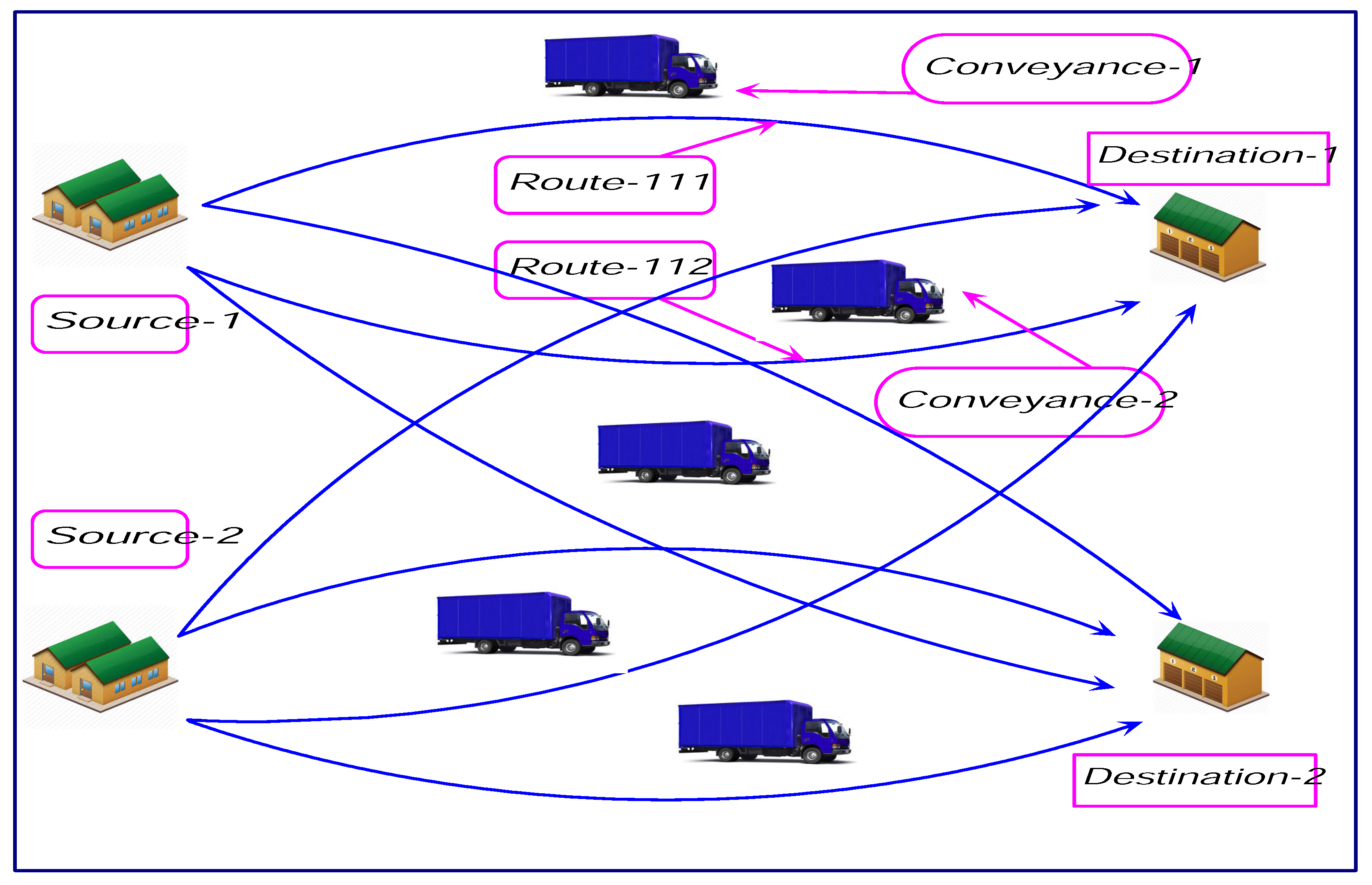
- The most important issues of this paper are to analyze how the travel distances are related to profit maximization when manufacturing companies transport both complementary and substitute items that are differentiated by distance including the fixed charge of the path and damageability. The importance of route on profit is illustrated.
- Until now, in transportation, no one has considered the space constraint at the destinations along with the budget constant. The idea of space constraint is introduced here.
- The earlier researchers gave attention to minimization of aggregate transportation expenditure and very few have realized the importance of consideration of total profit instead of total cost/expanses.
- As particular cases, several earlier transportation models are deduced from the present model.
1.2. Structure of the Paper
- Section 1: Introduction
- Section 2: Notations and Assumptions for the proposed model are given.
- Section 3: Model description and formulation
- Section 4: Numerical Experiments
- Section 5: Particular Cases
- Section 6: Sensitivity Analyses
- Section 7: A discussion of the models on the basis of numerical results are presented.
- Section 8: Practical implication is described.
- Section 9: Conclusions drawn.
1.3. Literature Review
1.4. Motivation
2. Notation and Assumptions
2.1. Notations
2.1.1. Parameters
- : quantity of homogeneous merchandise available at i-th source.
- : market demand at j-th goal.
- : actual demand at j-th goal.
- : quantity of the merchandise which can be carried by k-th conveyance along p-th route.
- : per unit transportation price from i-th origin to j-th goal by k-th vehicle via p-th route.
- : selling expenses at the j-th destination.
- : purchasing price at the i-th origin.
- : fixed transportation cost for shipping units from i-th source/origin to j-th goal/destination by k-th vehicles along p-th route.
- : rate of breakability per unit distance from i-th source to j-th goal via p-th route and k-th conveyance.
- : total budget at the j-th goal point.
- : distance from i-th origin to j-th goal along p-th route.
- : required space for r-th item.
- : available space to the j-th retailer.
- : power of the route length, related with the frangibility.
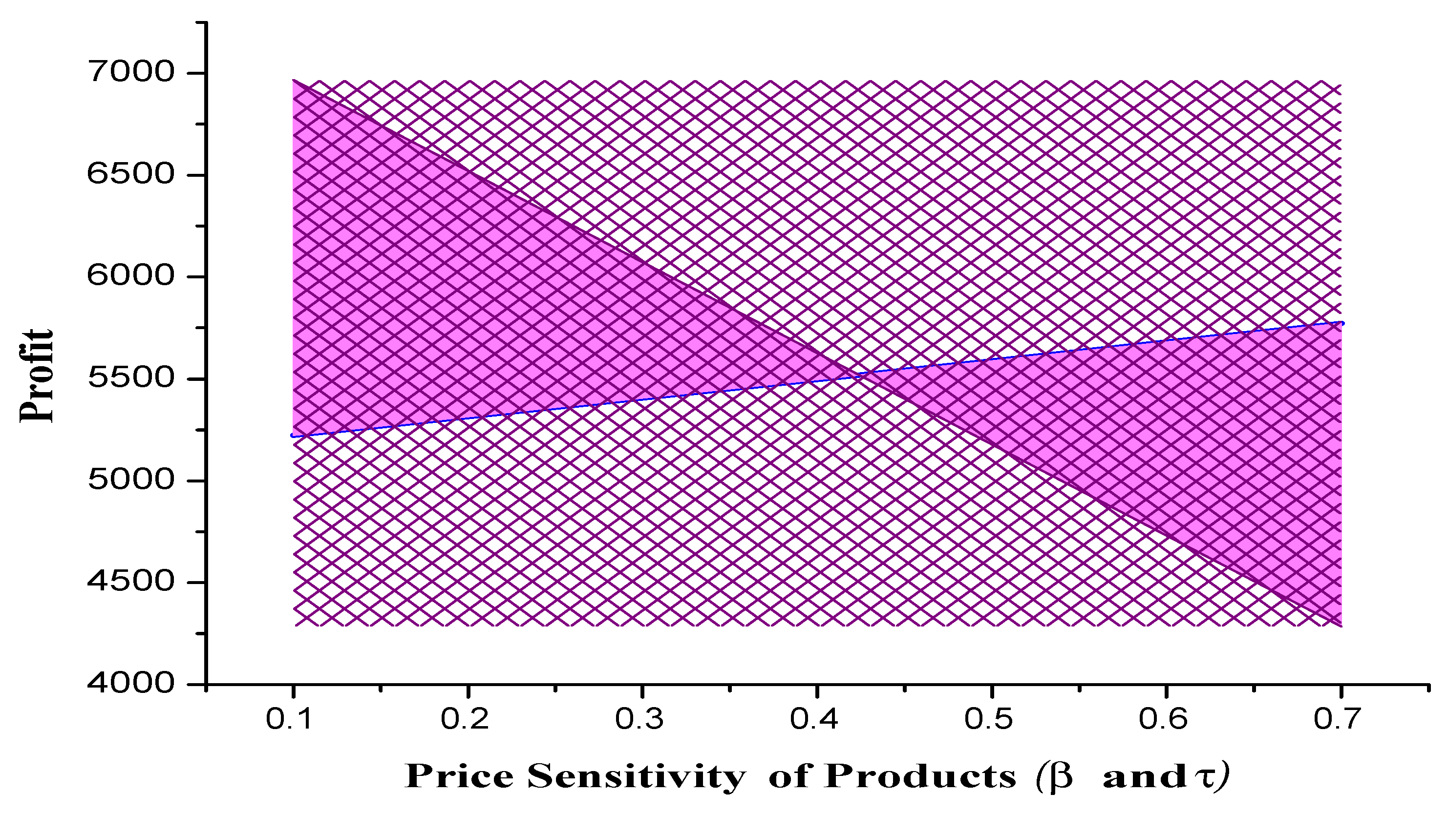
- , , and : Price sensitivity of products.
2.1.2. Decision Variable
- : the transported quantity from i-th source/origin to j-th goal/destination by k-th vehicle along p-th route (decision variable).
2.1.3. Indices
- R: total number of items.
- M: total number of origin/sources.
- N: total number of goal/destinations.
- L: total number of route/paths.
- K: total number of vehicles/conveyance.
2.2. Assumptions
- (i)
- Particulars are breakable and carried from sources to goals using a vehicle through a path. Broken/damaged amounts depend on conveyance and path.
- (ii)
- Particulars are substitutable and complementary to each other. In case of a substitute item, the demand is negative and is positive when the items are complementary nature:
3. Model Description and Formulation
3.1. Model-I: Crisp Model
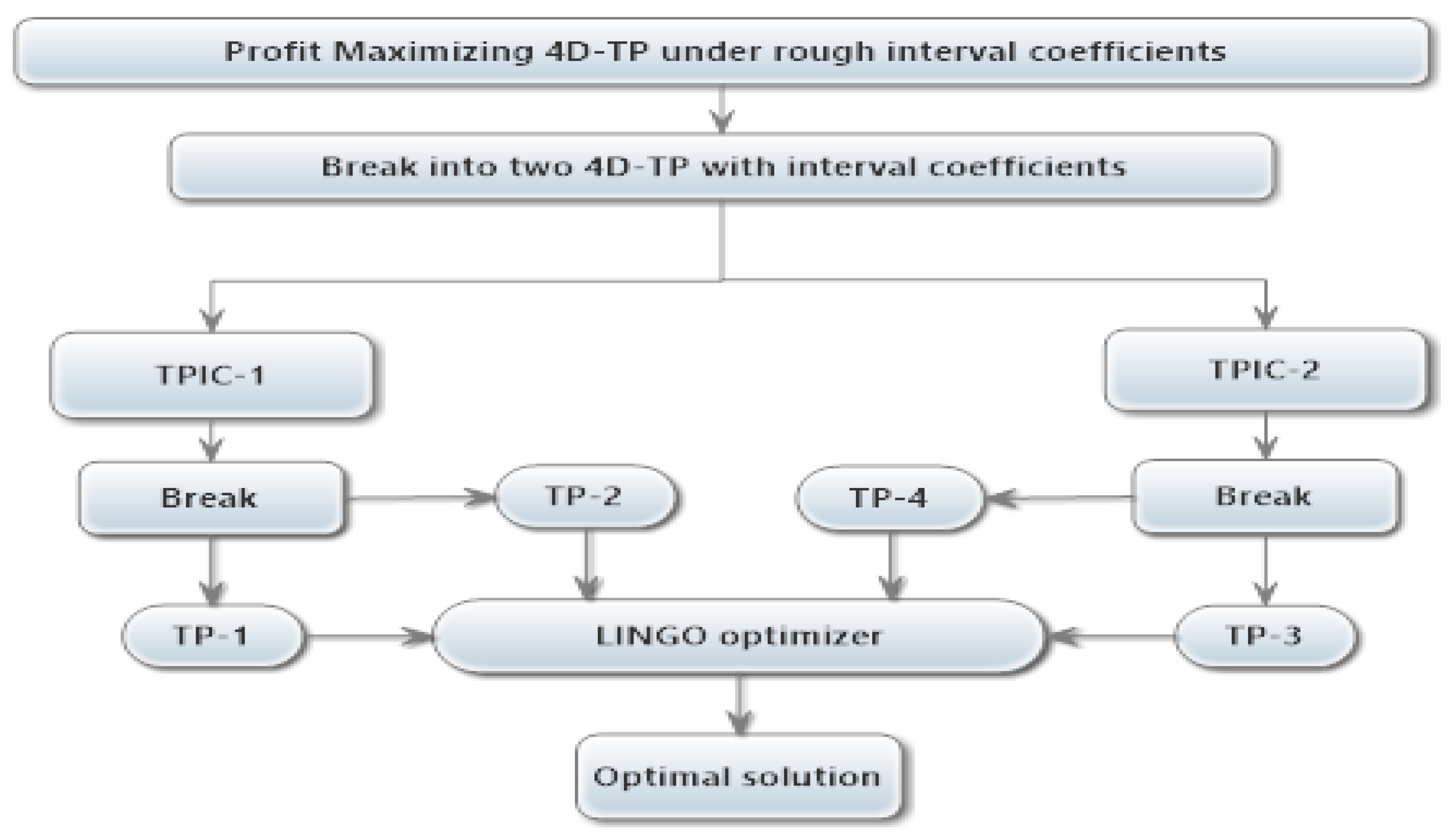
3.2. Model-II: Rough Model
3.3. The Mathematical Form of TPIC-1
3.4. The Mathematical Form of TPIC-2
3.4.1. TP-1
3.4.2. TP-2
3.4.3. TP-3
3.4.4. TP-4
3.4.5. Approach-2
4. Numerical Experiments
5. Particular Cases
5.1. Three-Dimensional TP Model
5.2. 2D-TP Model
5.3. 4D-TPs with Different Natures of the Items
6. Sensitivity Analyses
7. Discussion
7.1. Discussion for Particular Models
7.2. Results of Bera et al.’s Model
8. A Real-Life Problem
9. Conclusions
Author Contributions
Funding
Conflicts of Interest
Appendix A
Appendix A.1. Rough Intervals and Its Algebra
Appendix A.2. Expected Value of a Rough Interval (Shu and Edmund [38])
Appendix A.3. General Linear Programming Problem in Rough Interval Environments
Appendix A.3.1. LPIC-1
Appendix A.3.2. LPIC-2
Appendix A.3.3. Types of Solutions
- If LP-1 and LP-2 (LP-3 and LP-4) have optimal solutions, then the problem LPIC-1 (LPIC-2) has a finite bounded surely optimal (possibly optimal) range. If the maximizing value of LP-1 and LP-2 (LP-3 and LP-4) are respectively then the surely optimal range (possibly optimal range) of LPIC-1 (LPIC-2) is
- If LP-2 (LP-4) is unbounded, then LPIC-1 (LPIC-2) is unbounded.
- If LP-1 (LP-3) is infeasible, then LPIC-1 (LPIC-2) is infeasible.
Appendix A.4. Algorithm for Conversion from a Rough LPP to a Crisp LPP
- If LPIC-1 and LPIC-2 have an optimal range, then the LPRIC problem (1) has an optimal range which is a rough interval, compared to the surely optimal range
- If LPIC-1 has boundless range, then the LPRIC problem (1) has boundless range.
- If LPIC-2 is infeasible, then the LPRIC problem (1) has an infeasible solution space.
Appendix A.5. Convergence of the GRG Method
References
- Hitchcok, F.L. The distribution of a product form several sources to numerous localities. J. Math. Phys. 1941, 20, 224–230. [Google Scholar] [CrossRef]
- Schell, E.D. Distribution of a product by several properties. In Proceedings of the 2nd Symposium in Linear Programming, DCS/Comptroller, HQ US Air Force, Washington, DC, USA, 24–25 October 1955; pp. 615–642. [Google Scholar]
- Yang, L.; Liu, P.; Li, S.; Gao, Y.; Ralescu, D.A. Reduction methods of type-2 uncertain variables and their applications to solid transportation problem. Inf. Sci. 2015, 291, 204–237. [Google Scholar] [CrossRef]
- Kocken, H.G.; Sivri, M. A simple parametric method to generate all optimal solutions of fuzzy solid transportation problem. Appl. Math. Model. 2016, 40, 4612–4624. [Google Scholar] [CrossRef]
- Halder, S.; Das, B.; Panigrahi, G.; Maiti, M. Some special fixed charge solid transportation problems of substitute and breakable items in crisp and fuzzy environments. Comput. Ind. Eng. 2017, 111, 272–281. [Google Scholar] [CrossRef]
- Das, A.; Bera, U.K.; Maiti, M. A Profit Maximizing Solid Transportation Model Under a Rough Interval Approach. IEEE Trans. Fuzzy Syst. 2017, 25, 485–498. [Google Scholar] [CrossRef]
- Bera, S.; Giri, P.K.; Jana, D.K.; Basu, K.; Maiti, M. Multi-item 4D-TPs under budget constraint using rough interval. Appl. Soft Comput. 2018, 71, 364–385. [Google Scholar] [CrossRef]
- Sarkar, M.; Lee, Y.H. Optimum pricing strategy for complementary products with reservation price in a supply chain model. J. Ind. Manag. Optim. 2017, 13, 1553–1586. [Google Scholar] [CrossRef]
- Sarkar, M.; Hur, S.; Sarkar, B. Effects of Variable Production Rate and Time-Dependent Holding Cost for Complementary Products in Supply Chain Model. Math. Probl. Eng. 2017, 2017, 2825103. [Google Scholar] [CrossRef]
- Khanna, A.; Kishore, A.; Sarkar, B.; Jaggi, C. Supply Chain with Customer-Based Two-Level Credit Policies under an Imperfect Quality Environment. Mathematics 2018, 6, 299. [Google Scholar] [CrossRef]
- Hirsch, W.M.; Dantzig, G.B. The fixed charge problem. Naval Res. Logist. NRL 1968, 15, 413–424. [Google Scholar] [CrossRef]
- Kowalski, K.; Lev, B. On step fixed-charge transportation problem. Omega 2008, 36, 913–917. [Google Scholar] [CrossRef]
- Gen, M.; Li, Y.Z. Spanning tree-based genetic algorithm for bicriteria transportation problem. Comput. Ind. Eng. 1998, 35, 531–534. [Google Scholar] [CrossRef]
- Verma, R.; Biswal, M.P.; Biswas, A. Fuzzy programming technique to solve multi-objective transportation problems with some non-linear membership functions. Fuzzy Sets Syst. 1997, 91, 37–43. [Google Scholar] [CrossRef]
- Shafaat, A.; Goyal, S.K. Resolution of degeneracy in transportation problems. J. Oper. Res. Soc. 1988, 39, 411–413. [Google Scholar] [CrossRef]
- Saad, O.M.; Abbas, S.A. A parametric study on transportation problem under fuzzy environment. J. Fuzzy Math. 2003, 11, 115–124. [Google Scholar]
- Iqbal, M.W.; Sarkar, B. Recycling of lifetime dependent deteriorated products through different supply chains. RAIRO-Oper. Res. 2019, 53, 129–156. [Google Scholar] [CrossRef]
- Sarkar, B.; Mandal, B.; Sarkar, S. Preservation of deteriorating seasonal products with stock-dependent consumption rate and shortages. J. Ind. Manag. Optim. 2017, 13, 187–206. [Google Scholar] [CrossRef]
- Pramanik, S.; Maity, K.; Jana, D.K. A multi-objective solid transportation problem with reliability for damageable items in random fuzzy environment. Int. J. Oper. Res. 2018, 31, 1–23. [Google Scholar] [CrossRef]
- Sarkar, B.; Shaw, B.K.; Kim, T.; Mitali, S.; Shin, D. An integrated inventory model with variable transportation cost, two-stage inspection, and defective items. J. Ind. Manag. Optim. 2017, 13, 1975–1990. [Google Scholar] [CrossRef]
- Ojha, A.; Mondal, S.K.; Maiti, M. A solid transportation problem with partial nonlinear transportation cost. J. Appl. Comput. Math. 2014, 3, 1–6. [Google Scholar]
- Ishfaq, N.; Sayed, S.; Akram, M.; Smarandache, F. Notions of Rough Neutrosophic Digraphs. Mathematics 2018, 6, 18. [Google Scholar] [CrossRef]
- Bit, A.K.; Biswal, M.P.; Alam, S.S. Fuzzy programming approach to multiobjective solid transportation problem. Fuzzy Sets Syst. 1993, 57, 183–194. [Google Scholar] [CrossRef]
- Jiménez, F.; Verdegay, J.L. Solving fuzzy solid transportation problems by an evolutionary algorithm based parametric approach. Eur. J. Oper. Res. 1999, 117, 485–510. [Google Scholar] [CrossRef]
- Li, T.H.S.; Su, Y.T.; Lai, S.W.; Hu, J.J. Walking motion generation, synthesis, and control for biped robot by using PGRL, LPI, and fuzzy logic. IEEE Trans. Syst. Man Cybern. Part B Cybern. 2011, 41, 736–748. [Google Scholar] [CrossRef]
- Dey, A.; Pal, A.; Pal, T. Interval type 2 fuzzy set in fuzzy shortest path problem. Mathematics 2016, 4, 62. [Google Scholar] [CrossRef]
- Kundu, P.; Kar, S.; Maiti, M. Fixed charge transportation problem with type-2 fuzzy variables. Inf. Sci. 2014, 255, 170–186. [Google Scholar] [CrossRef]
- Tao, Z.; Xu, J. A class of rough multiple objective programming and its application to solid transportation problem. Inf. Sci. 2012, 188, 215–235. [Google Scholar] [CrossRef]
- Haley, K.B. New methods in mathematical programming—The solid transportation problem. Oper. Res. 1962, 10, 448–463. [Google Scholar] [CrossRef]
- Ojha, A.; Das, B.; Mondal, S.K.; Maiti, M. A multi-item transportation problem with fuzzy tolerance. Appl. Soft Comput. 2013, 13, 3703–3712. [Google Scholar] [CrossRef]
- Liu, P.; Yang, L.; Wang, L.; Li, S. A solid transportation problem with type-2 fuzzy variables. Appl. Soft Comput. 2014, 24, 543–558. [Google Scholar] [CrossRef]
- Giri, P.K.; Maiti, M.K.; Maiti, M. Fully fuzzy fixed charge multi-item solid transportation problem. Appl. Soft Comput. 2015, 27, 77–91. [Google Scholar] [CrossRef]
- Schittkiowski, K. On the convergence of a generalized reduced gradient algorithm for nonlinear programming problems. Optimization 1986, 17, 731–755. [Google Scholar] [CrossRef]
- Khanra, A.; Maiti, M.K.; Maiti, M. Profit maximization of TSP through a hybrid algorithm. Comput. Ind. Eng. 2015, 88, 229–236. [Google Scholar] [CrossRef]
- Manerba, D.; Mansini, R.; Riera-Ledesma, J. The traveling purchaser problem and its variants. Eur. J. Oper. Res. 2017, 259, 1–18. [Google Scholar] [CrossRef]
- Hamzehee, A.; Yaghoobi, M.A.; Mashinchi, M. Linear programming with rough interval coefficients. J. Intell. Fuzzy Syst. 2014, 26, 1179–1189. [Google Scholar]
- Rebolledo, M. Rough intervals—Enhancing intervals for qualitative modeling of technical systems. Artif. Intell. 2006, 170, 667–685. [Google Scholar] [CrossRef]
- Xiao, S.; Lai, E.M.K. A rough programming approach to power-balanced instruction scheduling for VLIW digital signal processors. IEEE Trans. Signal Process. 2008, 56, 1698–1709. [Google Scholar] [CrossRef]
- Chinneck, J.W.; Ramadan, K. Linear programming with interval coefficients. J. Oper. Res. Soc. 2000, 51, 209–220. [Google Scholar] [CrossRef]


| References’ | Different Kind of TP | Item | Fixed Charge | Space Constraint | Budget Constraint | Different Kind of Environment |
|---|---|---|---|---|---|---|
| Hitchcock et al. [1] | 2-dimension | one | × | × | - | crisp |
| Schell [2] | 3-dimension | one | × | × | - | crisp |
| Haley [29] | 3-dimension | one | × | × | - | crisp |
| Hirsch and Dantzig [11] | 2-dimension | one | ✓ | × | × | crisp |
| Verma et al. [14] | 2-dimension | one | × | × | × | fuzzy |
| Shafaat and Goyal [15] | 2-dimension | one | × | × | × | crisp |
| Saad and Abbas [16] | 2-dimension | one | × | × | × | fuzzy |
| Jimenez et al. [24] | 3-dimension | one | × | × | × | fuzzy |
| Tao et al. [28] | 3-dimension | one | × | × | × | rough |
| Ojha et al. [30] | 2-dimension | multi-item | × | × | ✓ | fuzzy |
| Liu et al. [31] | 3-dimension | one | × | × | × | type-2 fuzzy |
| Kundu et al. [27] | 3-dimension | multi-item | × | × | × | type-2 fuzzy |
| Yang et al. [3] | 2-dimension | one | ✓ | × | × | fuzzy |
| Giri et al. [32] | 3-dimension | multi-item | ✓ | × | × | fuzzy |
| Kocken et al. [4] | 3-dimension | one | × | × | × | fuzzy |
| Das et al. [6] | 3-dimension | one | × | × | × | rough |
| Present Paper | 4-dimensional | multi-item | ✓ | ✓ | ✓ | rough |
| p | 1 | 2 | |||||||
|---|---|---|---|---|---|---|---|---|---|
| k | 1 | 2 | 1 | 2 | |||||
| i/j | 1 | 2 | 1 | 2 | 1 | 2 | 1 | 2 | |
| Model-I | |||||||||
| (Crisp Model) | |||||||||
| 1 | 0.5 | 2.1 | 1.7 | 1.12 | 0.85 | 0.5 | 1.38 | 1.28 | |
| 2 | 1.21 | 1.28 | 2.05 | 0.6 | 1.65 | 2.72 | 1.66 | 1.78 | |
| 1 | 1.5 | 2.25 | 2.0 | 1.3 | 0.08 | 0.7 | 1.05 | 1.25 | |
| 2 | 1.05 | 2.15 | 2.2 | 0.9 | 1.35 | 2.25 | 1.85 | 0.98 | |
| 1 | 1.3 | 1.2 | 1.91 | 1.2 | 0.9 | 0.94 | 0.73 | 0.93 | |
| 2 | 1.22 | 1.3 | 2 | 0.7 | 1.8 | 3 | 1.8 | 1.8 | |
| 1 | 0.01 | 0.01 | 0.01 | 0.01 | 0.02 | 0.02 | 0.02 | 0.02 | |
| 2 | 0.01 | 0.01 | 0.01 | 0.01 | 0.02 | 0.02 | 0.02 | 0.02 | |
| 1 | 0.01 | 0.01 | 0.01 | 0.01 | 0.02 | 0.02 | 0.02 | 0.02 | |
| 2 | 0.01 | 0.01 | 0.01 | 0.01 | 0.02 | 0.02 | 0.02 | 0.02 | |
| 1 | 0.01 | 0.01 | 0.01 | 0.01 | 0.02 | 0.02 | 0.02 | 0.02 | |
| 2 | 0.01 | 0.01 | 0.01 | 0.01 | 0.02 | 0.02 | 0.02 | 0.02 | |
| 1 | 1.9 | 1.7 | 1.1 | 1.3 | 1.2 | 1.4 | 0.3 | 1.8 | |
| 2 | 1.2 | 1.85 | 0.9 | 1.5 | 1.5 | 2.1 | 2.1 | 1.6 | |
| Model-II | |||||||||
| (Rough Model) | |||||||||
| 1 | ([1, 2], | ([0.5, 1.5], | ([1.1, 2.3], | ([0.8, 1.3], | ([1.4, 2.3], | ([0.7, 1], | ([1.2, 2], | ([1.2, 2.4], | |
| [0.7, 2.3]) | [0.5, 2]) | [1, 2.5]) | [0.5, 2]) | [1.2, 2.8] ) | [0.5, 1.5]) | [1.2, 2.3]) | [1, 3]) | ||
| 2 | ([1.2, 2.5], | ([0.9, 2], | ([1.1, 2], | ([1, 2], | ([1.1, 2.2], | ([1, 2.5], | ([0.9, 2.1], | ([1.3, 2.5], | |
| [1, 3]) | [0.5, 3.2]) | [0.7, 2.5]) | [0.9, 2.6]) | [1, 2.7]) | [0.3, 3]) | [0.7, 2.8]) | [1.1, 3.5]) | ||
| 1 | ([1.3, 2.7], | ([1.7, 2.8], | ([1.5, 2.5], | ([1.6, 2.4], | ([1.3, 3], | ([1.4, 2], | ([1.5, 2.6], | ([1.8, 2.7], | |
| [1, 3]) | [1.2, 3.1]) | [1.4, 3.1]) | [1.5, 3.5]) | [1.2, 3.5]) | [1.1, 2.5]) | [1.3, 3]) | [1.6, 3.4] | ||
| 2 | ([1.5, 2.5], | ([1.3, 3], | ([1.7, 2.7], | ([1.4, 3], | ([2, 2.7], | ([1.3, 2.2], | ([1.6, 2.1], | ([1.6, 2.5], | |
| [1, 3.5]) | [1.1, 3.7]) | [1.5, 3]) | [1.2, 3.2]) | [1.8, 3]) | [1, 2.5]) | [1.5, 2.8]) | [1.4, 2.8]) | ||
| 1 | ([0.5, 1.5], | ([0.7, 1], | ([0.7, 1.3], | ([0.8, 1.6], | ([0.7, 1.4], | ([0.8, 1.8], | ([1, 1.5], | ([0.9, 1.8], | |
| [0.5, 2]) | [0.6, 1.5]) | [0.4, 2]) | [0.3, 1.7]) | [0.6, 2]) | [0.3, 2.3]) | [0.8, 1.8]) | [0.7, 2.1]) | ||
| 2 | ([0.2, 0.5], | ([0.3, 0.6], | ([0.9, 1.7], | ([1, 1.5], | ([0.9, 1.5], | ([0.5, 1.6], | ([0.4, 0.9], | ([1, 1.7], | |
| [0.1, 1]) | [0.2, 1]) | [0.6, 1.8]) | [0.5, 1.6]) | [0.4, 1.9]) | [0.2, 2]) | [0.2, 1]) | [0.5, 2]) | ||
| Models | Source | Demand | Capacities. of Conveyance. |
|---|---|---|---|
| -I | (90, 80, 85 | (75, 73, 70, | (90, 85, 80 |
| 85, 75, 70) | 65, 63, 60) | 85, 70, 75) | |
| {([89.5, 90], [88.6, 91]), | {([74, 75], [73.6, 76]), | {([89, 90], [88, 91]), | |
| ([79.6, 80], [78.5, 81.3]), | ([72.6, 73], [72, 74]), | ([84, 85], [83, 86.3]), | |
| ([84.7, 85], [83.5, 86]), | ([69.4, 70], [68.7, 71]), | ([79, 80], [78, 81.3]), | |
| -II | ([84.4, 85], [83.6, 86]), | ([64.5,65], [64, 66]), | ([84, 85], [83, 86.3]), |
| ([74, 75], [73.6, 76]), | ([62.4, 63], [62, 64]), | ([69, 70], [68, 71]), | |
| ([69.4, 70], [68.7, 71])} | ([59.4, 60], [59, 61])} | ([74, 75], [73, 76])} |
| Models | Purchasing Costs | Unit Selling Price | Budget | |
|---|---|---|---|---|
| -I | (9, 8, 10 | (52, 30, 24, | (3000, 2500, 2700) | (510, 520, 525) |
| 6, 7, 8.5) | 46, 28, 20) | |||
| {([8.3, 9], [8, 10]), | {([51.5, 52], [51, 53]), | {([8250,5000], | {([509.6,510.3], | |
| ([7.5, 8], [7, 9]), | ([29, 30], [28, 31]), | [7500,8600]), | [509, 511]), | |
| ([9, 10], [8, 10.5]), | ([23.5, 24], [23, 25]), | ([7500,8600], | ([519.4,520], | |
| -III | ([5.5, 6], [5, 7]), | ([45.5,45], [45.3, 46]), | [4500,4600]), | [519, 521]), |
| ([6.5, 7], [6, 7.8]), | ([27.4, 28], [27, 29]), | ([4400,4700]), | ([524, 525]), | |
| ([8, 8.5], [7.5, 9])} | ([19.5, 20], [19.1, 21])} | [4400,4700])} | [523,526])} |
| Route | Destination | Origin-1 | Origin-2 |
|---|---|---|---|
| 1 | 1 | 35 | 30 |
| 2 | 40 | 25 | |
| 2 | 1 | 30 | 35 |
| 2 | 25 | 30 |
| Models | Crisp Model | 4D Rough Model | |||
|---|---|---|---|---|---|
| TP-1 | TP-2 | TP-3 | TP-4 | ||
| Optimal profit | 6966.775 | 5293.95 | 8058.61 | 4109.11 | 9130.81 |
| Set-1 | Set-2 | Set-3 | Set-4 | ||
| x11111 = 63.07 | x11221 = 14.04 | x11122 = 48.7 | x11111 = 54.4 | x11111 = 52.44 | |
| x11122 = 52.75 | x12112 = 46 | x11221 = 65.3 | x11221 = 32.2 | x11112 = 25.41 | |
| x11222 = 8.75 | x12211 = 29.96 | x11222 = 49.6 | x11222 = 17.9 | x11222 = 19.9 | |
| x21121 = 67.15 | x21121 = 50.46 | x12211 = 22.1 | x12211 = 0.2 | x12112 = 9.09 | |
| x21122 = 47.1 | x21122 = 21.84 | x12221 = 42.2 | x21121 = 20.3 | x12211 = 62.24 | |
| x22211 = 27.74 | x21211 = 33.04 | x21111 = 44 | x21122 = 19.9 | x21121 = 54.71 | |
| x22212 = 39.9 | x21222 = 45.16 | x21121 = 9.80 | x22211 = 31.31 | x21122 = 65.91 | |
| x22213 = 26.9 | x21223 = 26.07 | x21123 = 14.80 | x22213 = 2.23 | x21123 = 27.09 | |
| x11213 = 7.9 | x21123 = 27.16 | x22123 = 23.80 | x22113 = 62.04 | x22123 = 15.09 | |
| x11123 = 15.91 | x11123 = 15.91 | x11123 = 15.91 | x22212 = 18.65 | x21113 = 28.51 | |
| others are zero | others are zero | x21122 = 33.4 | other are zero | x21211 = 8.29 | |
| x22212 = 14.9 | x22212 = 31.21 | ||||
| other are zero | other are zero |
| = 0.0 | = 0.2 | = 0.4 | = 0.5 | = 0.6 | = 0.8 | = 1.0 |
|---|---|---|---|---|---|---|
| 6351.76 | 6393.95 | 6412.61 | 6463.11 | 6488.81 | 6504.54 | 6523.54 |
| x11111 = 32.75 | x11111 = 32.84 | x11111 = 32.86 | x11111 = 28.85 | x11111 = 28.14 | x11111 = 28.09 | x11111 = 28.92 |
| x11222 = 30.33 | x11222 = 30.33 | x22212 = 27.46 | x11222 = 30.13 | x11222 = 30.02 | x11222 = 30.33 | x11222 = 30.33 |
| x12211 = 45.65 | x12211 = 45.576 | x12211 = 45.52 | x12211 = 45.5 | x12211 = 45.48 | x12211 = 45.44 | x12211 = 45.40 |
| x21121 = 52.20 | x21121 = 52.16 | x21121 = 52.13 | x21111 = 39.2 | x21113 = 39.09 | x21113 = 42.76 | x21113 = 42.76 |
| x21122 = 10.8 | x21122 = 18.75 | x21122 = 10.712 | x21121 = 32.3 | x21121 = 32.24 | x21121 = 54.05 | x21121 = 54.21 |
| x21223 = 30.74 | x21223 = 30.44 | x21223 = 30.04 | x21123 = 14.9 | x21123 = 14.71 | x21123 = 24.01 | x21123 = 24.32 |
| x22111 = 23.9 | x22111 = 23.13 | x22111 = 23.80 | x21222 = 23.14 | x21222 = 23.37 | x21222 = 23.41 | x21222 = 33.51 |
| x22213 = 32.9 | x22213 = 32.06 | x22213 = 32.16 | x22213 = 32.16 | x22213 = 32.22 | x22113 = 32.8 | x22113 = 41.05 |
| and all | and all | x22212 = 18.9 | x22212 = 27.46 | x21211 = 27.49 | and all | and all |
| others | others | and all others | and all | x22212 = 5.61 | others are zero | others are zero |
| variables | variables | variables | others | and all | ||
| are zero | are zero | are zero | variables | others are zero | ||
| are zero |
| Results without Space and Budget | Results with Space and without Budget | Results without Space and with Budget |
|---|---|---|
| x11111 = 42.75 | x11221 = 22.84 | x11211 = 19.06 |
| x11212 = 13.33 | x11222 = 32.04 | x21222 = 53.33 |
| x12211 = 25.65 | x12211 = 45.57 | x22212 = 14.9 |
| x21121 = 52.20 | x21121 = 52.16 | x21121 = 32.13 |
| x21122 = 10.8 | x21122 = 10.75 | x21122 = 10.71 |
| x21223 = 57.74 | x21223 = 30.44 | x21213 = 24.54 |
| x22112 = 43.9 | x22112 = 53.16 | x22112 = 53.80 |
| x22213 = 32.9 | x22213 = 32.16 | x22213 = 32.16 |
| x12213 = 12.9 | x12213 = 12.9 | x21122 = 27.4 |
| x11123 = 21.17 | x11123 = 11.17 | x11123 = 31.12 |
| and all others | and all others | and all others |
| variables are zero | variables are zero | variables are zero |
| Optimal profit 6579.135 | Optimal profit 6529.07 | Optimal profit 6513.513 |
| 823.76 | 1263.95 | 323.61 | 2623.21 |
|---|---|---|---|
| x1111 = 14.22 | x1111 = 0.82 | x1111 = 16.52 | x1111 = 18.04 |
| x1112 = 0.75 | x1112 = 4.19 | x1112 = 4.43 | x1112 = 9.12 |
| x1121 = 0.05 | x1121 = 6.26 | x1121 = 0.72 | x1121 = 0.21 |
| x1122 = 11.225 | x1122 = 12.06 | x1122 = 0.92 | x1122 = 11.42 |
| x1211 = 8.25 | x1211 = 0.36 | x1211 = 0.26 | x1211 = 0.53 |
| x1212 = 0.65 | x1212 = 0.16 | x1212 = 0.36 | x1212 = 0.43 |
| x1222 = 0.25 | x1222 = 5.06 | x1222 = 0.16 | x1221 = 8.12 |
| x2111 = 0.51 | x2111 = 0.06 | x2111 = 0.91 | x1222 = 0.09 |
| x2112 = 0.62 | x2112 = 8.03 | x2112 = 0.82 | x2111 = 5.05 |
| x2121 = 29.74 | x2121 = 0.4 | x2121 = 4.24 | x2112 = 27.3 |
| x2122 = 5.9 | x2122 = 0.44 | x2122 = 0.80 | x2121 = 8.44 |
| x2211 = 0.65 | x2211 = 5.26 | x2211 = 0.6 | x2122 = 5.32 |
| x2213 = 10.25 | x2213 = 0.96 | x2213 = 0.03 | x2213 = 14.76 |
| x2221 = 0.35 | x2221 = 4.81 | x2221 = 6.6 | x2212 = 5.75 |
| x2223 = 5.05 | x2223 = 5.76 | x2223 = 7.6 | x2223 = 9.2 |
| others zero | others zero | others zero | others zero |
| 623.76 | 1103.95 | 383.61 | 2056.32 |
|---|---|---|---|
| x1111 = 0.24 | x1111 = 0.84 | x1111 = 0.57 | x1111 = 14.17 |
| x1112 = 0.76 | x1112 = 0.11 | x1112 = 0.33 | x111 = 0.42 |
| x1121 = 0.05 | x1121 = 0.26 | x1121 = 0.62 | x1121 = 0.43 |
| x1122 = 0.24 | x1122 = 0.26 | x1122 = 0.92 | x1122 = 0.97 |
| x1211 = 0.23 | x1211 = 0.46 | x1211 = 0.36 | x1211 = 0.64 |
| x1212 = 0.54 | x1212 = 0.16 | x1212 = 0.46 | x1212 = 0.54 |
| x1222 = 0.25 | x1222 = 14.06 | x1222 = 0.26 | x1223 = 0.17 |
| x2111 = 0.51 | x2111 = 0.06 | x2111 = 0.91 | x1333 = 0.65 |
| x2112 = 0.62 | x2112 = 42.03 | x2112 = 0.82 | x1213 = 0.42 |
| x2121 = 32.74 | x2121 = 0.4 | x2121 = 44.24 | x2121 = 41.53 |
| x2122 = 20.9 | x2122 = 0.44 | x2122 = 0.80 | x2122 = 10.42 |
| x2211 = 7.65 | x2211 = 10.26 | x2211 = 0.6 | x2211 = 0.95 |
| x2213 = 0.25 | x2213 = 0.96 | x2213 = 0.03 | x221 = 0.94 |
| x2221 = 0.35 | x2221 = 25.11 | x2221 = 1.6 | x2221 = 0.79 |
| x2223 = 0.05 | x2223 = 8.76 | x2223 = 12.6 | x2222 = 0.57 |
| others zero | others zero | others zero | others zero |
| 4113.06 | 8093.95 | 453.61 | 8243.93 |
|---|---|---|---|
| x111 = 63 | x111 = 64.82 | x111 = 63.32 | x111 = 62 |
| x112 = 52 | x112 = 19.26 | x112 = 2.62 | x112 = 17.2 |
| x121 = 50.0 | x121 = 16.36 | x121 = 0.67 | x211 = 8 |
| x122 = 5.0 | x122 = 0.70 | x122 = 0.32 | x223 = 23 |
| x211 = 6 | x211 = 23.8 | x211 = 2.18 | x222 = 26.21 |
| x213 = 5.5 | x213 = 5.0 | x213 = 2.23 | other zero |
| x221 = 16.5 | x221 = 8.0 | x221 = 4.15 | |
| x223 = 19.5 | x223 = 27.4 | x223 = 4.32 | |
| other zero | other zero | other zero |
| Problem | Independent | Substitute | Complementary | Profit for Model-1 |
|---|---|---|---|---|
| 1 | Item-1, Item-2, Item-3 | 7388.841 | ||
| 1 | Item-1, Item-2 | Item-3 | 6966.775 | |
| 2 | Item-1, Item-2 | 5497.527 | ||
| 3 | Item-1, Item-3 | 6021.859 | ||
| 4 | Item-2, Item-3 | 5952.067 |
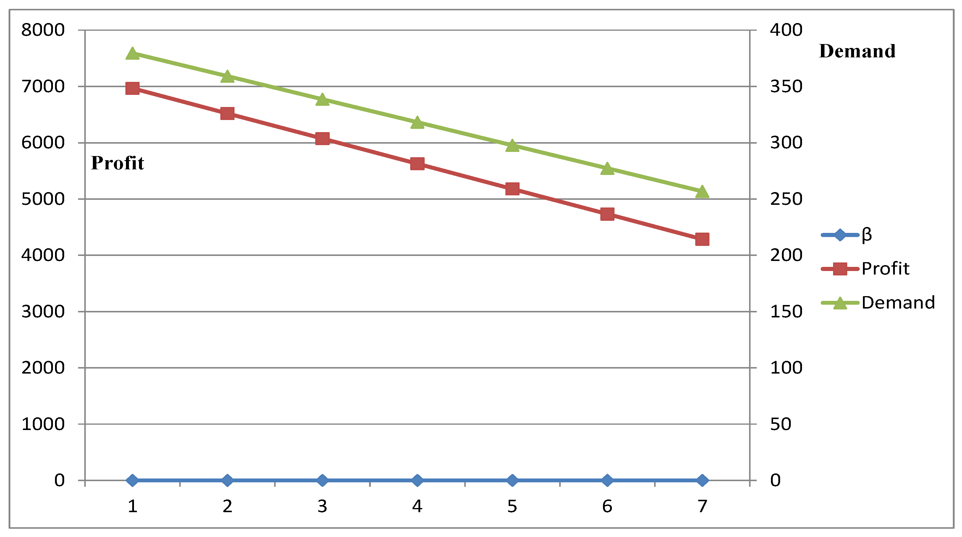
| Set | Maximum Profit | Demand | |||
|---|---|---|---|---|---|
| 1 | 0.052 | 0.052 | 0.1 | 6966.68 | 379.542 |
| 0.052 | 0.052 | 0.2 | 6519.775 | 359.084 | |
| 0.052 | 0.052 | 0.3 | 6072.868 | 338.627 | |
| 0.052 | 0.052 | 0.4 | 5625.962 | 318.1696 | |
| 0.052 | 0.052 | 0.5 | 5179.055 | 297.712 | |
| 0.052 | 0.052 | 0.6 | 4732.149 | 277.254 | |
| 0.052 | 0.052 | 0.7 | 4285.242 | 256.79 |
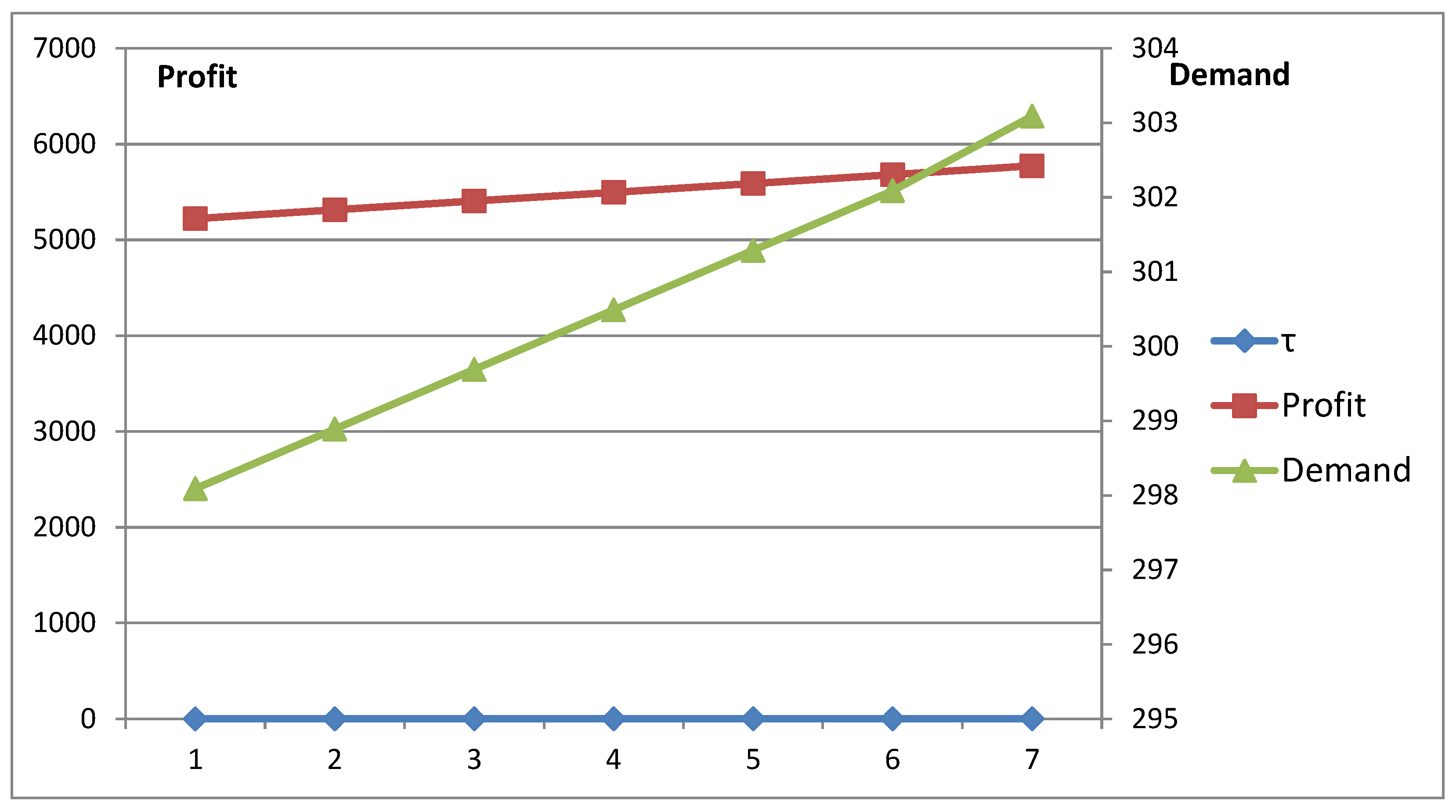
| Set | Maximum Profit | Demand | |||
|---|---|---|---|---|---|
| 1 | 0.1 | 0.052 | 0.5 | 5223.015 | 298.09 |
| 0.2 | 0.052 | 0.5 | 5314.598 | 298.89 | |
| 0.3 | 0.052 | 0.5 | 5406.181 | 299.69 | |
| 0.4 | 0.052 | 0.5 | 5497.76 | 300.49 | |
| 0.5 | 0.052 | 0.5 | 5589.34 | 301.29 | |
| 0.6 | 0.052 | 0.5 | 5680.93 | 302.09 | |
| 0.7 | 0.052 | 0.5 | 5772.513 | 303.89 |
| p | 1 | 2 | |||||||
|---|---|---|---|---|---|---|---|---|---|
| 1 | 2 | 1 | 2 | ||||||
| 1 | 2 | 1 | 2 | 1 | 2 | 1 | 2 | ||
| Model-I | |||||||||
| (Crisp Model) | |||||||||
| 1 | 0.15 | 1.1 | 1.2 | 0.12 | 0.85 | 0.5 | 1.38 | 1.28 | |
| 2 | 0.21 | 1.3 | 2.5 | 0.6 | 1.65 | 1.72 | 0.66 | 0.78 | |
| 1 | 1.5 | 2.25 | 2.0 | 1.3 | 0.08 | 0.7 | 1.05 | 1.25 | |
| 2 | 0.25 | 0.25 | 1.2 | 1.9 | 1.35 | 1.25 | 1.85 | 0.98 | |
| 1 | 1.3 | 1.2 | 1.91 | 1.2 | 0.9 | 0.94 | 0.73 | 0.93 | |
| 2 | 0.52 | 1.53 | 1.2 | 0.7 | 1.8 | 0.53 | 1.9 | 0.98 | |
| 1 | 0.01 | 0.01 | 0.02 | 0.03 | 0.01 | 0.02 | 0.01 | 0.02 | |
| 2 | 0.02 | 0.01 | 0.03 | 0.04 | 0.02 | 0.01 | 0.03 | 0.02 | |
| 1 | 0.04 | 0.03 | 0.01 | 0.02 | 0.05 | 0.01 | 0.02 | 0.03 | |
| 2 | 0.05 | 0.04 | 0.02 | 0.03 | 0.02 | 0.01 | 0.03 | 0.02 | |
| 1 | 0.01 | 0.01 | 0.01 | 0.01 | 0.02 | 0.02 | 0.02 | 0.02 | |
| 2 | 0.04 | 0.05 | 0.02 | 0.03 | 0.01 | 0.02 | 0.04 | 0.02 | |
| 1 | 1.1 | 1.4 | 1.5 | 1.0 | 1.2 | 1.4 | 0.3 | 1.8 | |
| 2 | 1.3 | 1.5 | 0.9 | 1.1 | 1.3 | 2.1 | 2.1 | 1.02 | |
| Models | Source | Demand | Capacities. of Conveyance. | Purchasing Costs | Unit Selling Price |
|---|---|---|---|---|---|
| -I | (85, 75, 80 | (60, 70, 75, | (86, 89, 90 | (45, 48, 51 | (132, 145, 124, |
| 83, 72, 68) | 62, 64, 59) | 81, 65, 70) | 36, 47, 58.5) | 126, 135, 137) |
© 2019 by the authors. Licensee MDPI, Basel, Switzerland. This article is an open access article distributed under the terms and conditions of the Creative Commons Attribution (CC BY) license (http://creativecommons.org/licenses/by/4.0/).
Share and Cite
Halder Jana, S.; Jana, B.; Das, B.; Panigrahi, G.; Maiti, M. Constrained FC 4D MITPs for Damageable Substitutable and Complementary Items in Rough Environments. Mathematics 2019, 7, 281. https://doi.org/10.3390/math7030281
Halder Jana S, Jana B, Das B, Panigrahi G, Maiti M. Constrained FC 4D MITPs for Damageable Substitutable and Complementary Items in Rough Environments. Mathematics. 2019; 7(3):281. https://doi.org/10.3390/math7030281
Chicago/Turabian StyleHalder Jana, Sharmistha, Biswapati Jana, Barun Das, Goutam Panigrahi, and Manoranjan Maiti. 2019. "Constrained FC 4D MITPs for Damageable Substitutable and Complementary Items in Rough Environments" Mathematics 7, no. 3: 281. https://doi.org/10.3390/math7030281
APA StyleHalder Jana, S., Jana, B., Das, B., Panigrahi, G., & Maiti, M. (2019). Constrained FC 4D MITPs for Damageable Substitutable and Complementary Items in Rough Environments. Mathematics, 7(3), 281. https://doi.org/10.3390/math7030281