Risk Measurement of Stock Markets in BRICS, G7, and G20: Vine Copulas versus Factor Copulas

Abstract

Multivariate copulas have been widely used to handle risk in the financial market. This paper aimed to adopt two novel multivariate copulas, Vine copulas and Factor copulas, to measure and compare the financial risks of the emerging economy, developed economy, and global economy. In this paper, we used data from three groups (BRICS, which stands for emerging markets, specifically, those of Brazil, Russia, India, China, and South Africa; G7, which refers to developed countries; and G20, which represents the global market), separated into three periods (pre-crisis, crisis, and post-crisis) and weighed Value at Risk (VaR) and Expected Shortfall (ES) (based on their market capitalization) to compare among three copulas, C-Vine, D-Vine, and Factor copulas. Also, real financial data demonstrated that Factor copulas have stronger stability and perform better than the other two copulas in high-dimensional data. Moreover, we showed that BRICS has the highest risk and G20 has the lowest risk of the three groups.

1. Introduction

The financial crisis of 2008 is considered by many economists as the worst financial crisis since the Great Depression of the 1930s. Consequences of the crisis were not only production curtailment but also difficulty for companies in external finance accessibility. One of the main reasons for this catastrophe was the underestimation of risk (see Jickling (2009) [1] and Salmon et al. (2012) [2]). Therefore, study risk measurement would be able to prevent or give a signal to avoid huge potential loss. Diverse markets lead to different risks (see Luo et al. (2015) [3], Shahzad et al. (2018) [4], Airouss et al. (2018) [5], and others), and according to Zhang & Zheng (2018) [6] and Wang et al. [7], there is a huge difference in stock markets and banks between emerging markets and advanced countries, especially in terms of seasonality. Also, different countries have different levels of influence on the global economic performance (see Zhang (2018) [8] and Amavilah (2017) [9]). Furthermore, Salachas et al. (2017) [10], Tsai (2015) [11], and Mustafa et al. (2015) [12] revealed the structural changes or differences among pre-crisis, crisis, and post-crisis periods via monetary policy, the connection between the oil price and the stock market, and the flight-to-quality between stock and bond markets. Therefore, measuring and comparing financial risks among BRICS (Brazil, Russia, India, China, and South Africa), G7, and G20 in different periods has important value in both practical and academic aspects. On the micro level, it is also meaningful for financial institutions, investors, and government departments to study risk measurement, thereby avoiding great loss and financial storm.

Dependence analysis of the financial market is important for effective diversification in risk management. Since the invention of copula by Sklar [13], several researchers had made contributions to develop the copula structure from bivariate copulas, multivariate copulas to Vine copulas, hierarchical Archimedean copulas, Factor copulas, and so on. Because of the advantage in dependence measurement of copulas, copula-based methods have been commonly used to measure the dependence structure between financial assets for their characteristics. Kaishev et al. (2007) [14] analyzed the impact of survival functions and related indexes, expectations of life, and annuity values by bivariate copulas; Li (1999) [15] introduced multivariate copulas for analyzing default correlation. Berger and Missong (2014) [16] adopted elliptical copulas and Value at Risk (VaR) to give advice for financial crises. So and Yeung (2014) [17] investigated a time varying conditional dependence by vine decomposition via the Vine-GARCH model. Mejdoub and Arab (2018) [18] tested the sensitivity of capital requirement to the dependence structure through D-Vine copulas. Pourkhanali et al. (2016) [19] discovered that the second tier financial institutions pay a larger contribution to the systemic risk by C-Vine and D-Vine copulas. Aloui and Aïssa (2016) [20] demonstrated the dynamic relationship among the energy, stock, and currency markets by Vine copulas. Besides, various Vine-based approaches have been adopted to solve problems like system risk, VaR, financial crisis, dynamic correlation (see Pourkhanali et al. (2016) [19], Reboredo and Ugolini (2015) [21], and Huang et al. (2009) [22], So and Yeung (2014) [17]). Moreover, Hierarchical Archimedean was introduced, and it was adopted to study portfolio credit risk (see Okhrin (2013) [23], Mai and Scherer (2012) [24], and Hering et al. (2010) [25]).

According to previous literature review, copula-based methods have been widely applied to investigate the correlation structure of financial markets and risk measurement. Besides, Oh and Patton (2017) [26] and Wu et al. (2012) [27] pointed out that copulas can accurately measure nonlinear correlations and tail dependence, so they can measure financial risk more precisely than multivariate distributions. However, there are still some limitations. First, bivariate copulas can capture nonlinear correlations and asymmetric tail dependence, but they utilize information from only two variables (see Kaishev et al. (2007) [14] and Craiu and Sabeti (2012) [28]). Second, multivariate copulas, such as multivariate Gaussian, multivariate Frank, multivariate Gumbel, and multivariate Clayton copulas, may be able to measure nonlinear dependence, but they are not flexible (see Li (1999) [15] and Kole et al. (2007) [29]). Third, in hierarchical dependence structure for Archimedean copulas, variables are clustered more closely. So, this structure tends to be restrictive(see Joe (2014) [30]), and it is driven by one single parameter, which limits the flexibility of the model (see Okhrin and Tetereva (2017) [31]). Fourth, Vine copulas are more flexible than multivariate copulas (see Aas et al. (2009) [32] and Haff et al. (2016) [33]). However, we found that most of the papers that adopted Vine copulas have tended to use low dimensional data. As the number of dimensions grows, the dependence parameters of Vine copulas (O(d${}^2$)) increase exponentially, where d is the number of variables, and this will undoubtedly increase the calculations. Fourth, few papers have used Vine copulas to deal with data with more than 12 dimensions.Therefore, the above-mentioned copula models are not really flexible and are not easy to estimate with high dimensional data.

A recent model, named Factor copulas, may help to fix these drawbacks. To avoid the larger number of dependence parameters and huge calculation time, Krupskii and Joe (2013) proposed the Factor copula model. Factor copulas are reliable on high-dimensional data, and they have fewer dependence parameters and, therefore, a reduced calculation process [34]. Meanwhile, Oh and Patton (2017) proposed an alternate way to construct the Factor copulas that enables the Factor copulas to link observed data to latent variables, which makes the results easier to interpret. Besides, factor copulas may be better-fitted than Vine copulas due to their simpler dependence structure, and they may be better than the classical copula models because of tail dependence [26]. Because of the large span of data dimensions (from 5 to 19), there are different levels of development (from emerging markets to advanced countries) and complexity of various endogenous and exogenous variables, so Factor copulas may be a better choice. In this paper, Factor copulas were adopted to estimate the sensitivity of each country to latent variables, and VaR and ES were derived by Vine and Factor copulas. A comparison of VaR and Expected Shortfall (ES) between Factor and Vine copulas determined the better method for risk measurement; therefore, more reliable results could be given to cope with the potential risks.

First, we proposed the factor copula-GARCH models to measure the dependence structures of stock returns and latent economic factors. The factor copula-GARCH models are able to capture the potential skewness and kurtosis of stock returns, as well as asymmetric dependence and tail dependence between stock returns and latent economic factors. These merits were conducive to the measurement of stock market risk. Countries like France, Germany, and Italy had larger coefficients of latent variables, which implies that they are more sensitive to the latent economic factors. China and Saudi had the lowest coefficients, which means that they are less vulnerable during crisis periods. Second, G20 had the lowest risk and BRICS had the highest, implying that, with economic globalization, diversified investment could reduce risk. Third, the gap in potential risk between G7 and G20 widened from pre-crisis to post-crisis, which means that emerging markets are playing a greater role in the global economy and are mitigating the risk from G7 countries in global markets. Fourth, pre-crisis results using Factor copula models revealed strong correlations among most of the countries, and this may be an early alarm for an upcoming financial crisis.

The remainder of the paper is structured as follows: Section 2 presents the data description. Section 3 presents the definition of the GARCH model, Vine and Factor copulas, VaR, and ES. Section 4 describes an empirical study of daily returns of stock indexes of BRICS, G7, and G20. Section 5 gives a brief conclusion and a discussion of further research.

2. Methodology

Firstly, ARMA(1,1)-GJR-GARCH(1,1) models using four different distributions (normal, skew- norm, skew-t and skew-ged) in the three periods were applied to get the cumulative distribution function (CDF), and the most suitable distribution was selected by AIC and BIC. Considering the problem of modeling the joint distribution of time series data by copulas, we followed the two-step estimation [35]. We estimated the conditional marginal distribution by the ARMA-GJR-GARCH model and obtained the parameters, including the leverage effect, at the first step. Then, we estimated C-Vine, D-Vine, and Factor copulas separately. As for VaR and ES, we conducted 10,000 simulations using the three methods for the three periods; then, we assumed that the copula structure is constant during each period and adopted the rolling window model to estimate copula estimators. Finally, we obtained the VaR and ES and compared the three methods. In this section, we briefly introduce the ARMA-GARCH model, Vine copulas, Factor copulas, tail dependence, VaR, and ES.

2.1. ARMA-GJR-GARCH

The ARMA-GJR-GARCH model that we used was presented by Harvey and Todd [36] as the ARMA(1,1):

$$\begin{array}{c}\hfill y_t=c+\phi y_{t-1}+\rho {\epsilon }_{t-1}+{\epsilon }_t,\end{array}$$

(1)

where y${}_t$ is the conditional mean, and $\epsilon$${}_t$ is the error term. Additionally, the conditional variance model GJR-GARCH(1,1) is defined as:

$$\begin{array}{c}\hfill {\sigma }_t^2=\omega +(\alpha +\gamma {\mathbb{I}}_{t-1}){\epsilon }_{t-1}^2+\beta {\sigma }_{t-1}^2,\end{array}$$

(2)

where

$${\mathbb{I}}_{t-1}=\left\{\begin{array}{cc}0\hfill & \mathrm{if}{\epsilon }_{t-1}\ge 0,\hfill \\ 1\hfill & \mathrm{if}{\epsilon }_{t-1}<0.\hfill \end{array}\right.$$

$\gamma$ is the leverage effect; $\epsilon$${}_t$ = $\sigma$${}_t$$\eta$${}_t$ and $\eta$${}_t$ are i.i.d. variables of standard innovation.

We can get the parameters of GARCH model by maximizing the log likelihood and then getting its CDFs by transformation. Similarly, we used MLE to estimate the parameters of copulas with CDFs obtained from the GARCH model. Marginal distributions were selected among the skew-generalized error distribution, skewed-t distribution, skew-normal distribution, and generalized error distribution by AIC and BIC. Due to space limitations, selections of CDFs of each country during each period are not listed.

2.2. Vine Copula and Factor Copula Models

A copula is a tool to build a multivariant joint distribution from marginal distributions. Copulas are becoming more popular, since they lose the constraint of independent assumption. Briefly speaking, let F${}_X$ be the CDF of X, assume that X = (X${}_1$, X${}_2$, ⋯, X${}_n$), and F${}_{Xj}$ is the marginal distribution of X${}_j$ for j = 1, ⋯, n. According to Sklar [13], if the margins are continuous on their domain, then a copula can build a unique joint distribution function, which is F${}_X$(x${}_1$, x${}_2$, ⋯, x${}_n$) = C${}_X$(F${}_{X1}$, ⋯, F${}_{Xn}$). Also, copulas are suitable for modeling data with tail dependence and asymmetry. Tail dependence is used in extreme value theory, which allows us to obtain the characteristic of tail implied by a given Factor copula model. The definitions of tail dependence for two variables with marginal distribution F${}_i$,F${}_j$ are:

$${\tau }_{ij}^L\equiv \underset{q\to 0^{+}}{lim}{\displaystyle \frac{Pr[X_i⩽F_i^{-1}\left(q\right),X_j⩽F_j^{-1}\left(q\right)]}{q}}$$

(3)

$${\tau }_{ij}^U\equiv \underset{q\to 1^{-}}{lim}{\displaystyle \frac{Pr[X_i>F_i^{-1}\left(q\right),X_j>F_j^{-1}\left(q\right)]}{1-q}}.$$

(4)

In the following paragraph, the sequence of Vine copulas is ordered by tail dependence.

2.2.1. Vine Copulas

The basic idea of Vine copulas is to decompose a d-dimensional copula density into a pair-copula by conditioning such that it can help to reduce the number of dimensions and get the result. It is noteworthy to mention that there are different ways to decompose the density function. In this paper, we adopted C-Vine and D-Vine copulas and selected the sequence by empirical Kendall’s tau. A graph of four-dimensional tree decomposition of C-Vine and D-Vine is shown in Figure 1.

Firstly, we calculated the empirical Kendall’s tau of each pair. For C-Vine, we calculated each variable’s summation of its tau and then picked the variable with the greatest value as the first sequence. For example, there are four variables: W, X, Y, and Z. We calculated the summation of the empirical Kendall’s tau $\tau$${}_w$ of W and X, W and Y, and W and Z. Similarly, this was done for $\tau$${}_x$, $\tau$${}_y$, and $\tau$${}_z$. Then, we set the variable with the biggest $\tau$ as the first sequence. Then, we calculated the $\tau$ of the remaining variables and set the second order. This was repeated until we got the whole sequence. For D-Vine, we picked the pair with the greatest tau, and found the second biggest pair of these two variables and set the variable with a smaller tau with the other variables as the first sequence. Then, we ordered the third sequence by the largest tau with the second variable without the ordered one. We use a four-variable selection as an example. If the tau between W and X is the greatest among all pairs, and the second biggest of W is W and Y $\tau$${}_{w,y}$, for X, it is Z, $\tau$${}_{x,z}$. If $\tau$${}_{w,y}$ < $\tau$${}_{x,z}$, then we set W as the first sequence, X as the second, and then find the biggest tau among the rest of the variables and set it as the third. We repeated this step until we had obtained the complete sequence.

2.2.2. Factor Copulas

Vine copulas provide an idea to decompose multi-dimensional data into pairs, but can also cause the calculation problem. Factor copulas, as one of the latest models, have several advantages such as a simpler calculation process, and the results can be explained easily and nicely. To be specific, stock indexes are not only influenced by endogenous variables but also by exogenous variables like interest rate, political stability, and weather. While these exogenous variables cannot be neglected and measured, Factor copulas provide a way that we can treat all of these variables as latent variables such that we can get a better result.

After we have transformed the marginal distribution into a uniform distribution, that is, F${}_{Xi}$ = u${}_i$∼U (0, 1), we get the uniform random variable vector U = (U${}_1$, ⋯, U${}_n$). Here, we adopted the Factor copula model proposed by Joe Harry from several Factor copula models (such as Hull and White [37], Oh and Patton [26], Vasicek [38], etc.) due to its simplicity and traceability on parameter estimation processes. Then, the Joint CDF C(u${}_1$, ⋯, u${}_n$) could be built by U. Given p latent variables V${}_1$, ⋯, V${}_p$ and without generality, we assumed that every latent variable was i.i.d and uniformly distributed. Then, we were able to get the Factor copula model (5),

$$\begin{array}{c}\hfill C(u_1,\cdots ,u_n)={\int }_{{[0,1]}^p}\prod _{j=1}^n{F}_{j|V_1,\cdots ,V_p}\left(u_j\right|v_1,\cdots ,v_p)d{v}_1\cdots d{v}_p.\end{array}$$

(5)

When p = 1, there is only one latent variable. C${}_{j,V_1}$ represents the joint CDF of (U${}_j$, V${}_1$), while c${}_{j,V_1}$ pdf. Since F${}_{j|V_1}$ = C${}_{j|V_1}$(u${}_j$|v${}_1$) = ∂C${}_{j,v_1}$(u${}_j$,v${}_1$)/∂v${}_1$, then Equation (3) becomes:

$$\begin{array}{c}\hfill C(u_1,\cdots ,u_n)={\int }_0^1\prod _{j=1}^n{F}_{j|V_1}\left(u_j\right|v_1)d{v}_1={\int }_0^1\prod _{j=1}^n{C}_{j|V_1}\left(u_j\right|v_1)d{v}_1.\end{array}$$

(6)

Then the likelihood can be written as:

$$\begin{array}{c}\hfill L(u_1,\cdots ,u_n;\theta )=\prod _{i=1}^{n}c(u_1,\cdots ,u_n;\theta ).\end{array}$$

(7)

The Gauss–Legendre quadrature approach performs well in approximation by replacing the integral as a summation of the weighted integrands at the quadrature points. The Gauss–Legendre formula is,

$$\begin{array}{c}\hfill c(u_1,\cdots ,u_n;\theta )\approx \sum _{k=1}^{n_q}{\omega }_k\prod _{j=1}^n{c}_{j,V_1}(u_j,x_k;{\theta }_j),\end{array}$$

(8)

where w${}_k$ stands for the quadrature weights, n${}_q$ is the number of quadrature points, and x${}_k$ is the nodes.

After obtaining the coefficients, we generated 10,000 simulations.Then, we added weights to each country’s simulations, and got the weighted log-return predictions, that is,

$$\begin{array}{c}\hfill \overline{Rt}=\sum _{i=1}^n\left(X_i{W}_i\right)/{\sum }_{i=1}^n{W}_i,\end{array}$$

(9)

where X${}_i$ stands for countries contained in the studied group, ${}_i$ is the corresponding market capitalization, and n = 5 for BRICS, n = 7 for G7, and n = 19 for G20. Similarly, we were able to get the real weighted log-returns. After that, we simply obtained the VaR and ES from the simulations.

2.3. Value at Risk

VaR is widely used in many areas to quantify the level of risk, and it was adopted by the Basel Committee for a long time. VaR can be explained intuitively and easily, and it is still a popular measurement in risk management. Mathematically, VaR is defined as:

$$\begin{array}{c}\hfill Va{R}_{\alpha }\left(X\right)=inf\{x\in \mathbb{R}:\mathbb{P}(r_t<x)>\alpha \},\end{array}$$

(10)

where $\alpha$∈ (0, 1) is the quantile, r${}_t$ is the return, and VaR means the occurrence of the losses at the $\alpha$ quantile.

Every $R_{t+i}$ can be obtained by simulations of different quantiles based on the historical information of Vine and Factor copula GJR-GARCH models.

In order to evaluate the different forecasting method, three methods of statistical backtesting are applied to measure the absolute amount of misspecifications, which are unconditional coverage (UC), independence (IND), and conditional coverage (CC) test. The LR${}_{UC}$, proposed by Kupiec (1995) [39], checks whether the rate of exceedances of a VaR model is statistically different from its realized rate:

$$\begin{array}{c}\hfill L{R}_{UC}=-2Ln{(1-P)}^{T-x}\ast P^x+2\ast Ln{\left({\displaystyle \frac{1-x}{T}}\right)}^{T-x}\ast {\left({\displaystyle \frac{x}{T}}\right)}^x,\end{array}$$

(11)

where x is the number of outliers, and T stands for the total number of predictions. And a likelihood ratio statistic method proposed by Christoffersen (1998) [40], aims to test if the misspecifications are correlated in time. The likelihood ratio is defined as:

$$\begin{array}{c}\hfill L{R}_{IND}=-2Ln\left[{(1-\pi )}^{N_{00}+N_{01}}{\pi }^{N_{01}+N_{11}}\right]+2Ln\left[{(1-{\pi }_{01})}^{N_{00}}{\left({\pi }_{01}\right)}^{N_{01}}{(1-{\pi }_{11})}^{N_{10}}{\pi }_{11}^{N_{11}}\right],\end{array}$$

(12)

where N${}_{ij}$ is the number of observed values i followed by j, 1 represents a misspecification, and 0 a correct estimation. $\pi$ represents the probability of observing an exceedance, where ${\pi }_{ij}$ is the conditional probability, ${\pi }_{ij}=\frac{N_{ij}}{\sum _j{N}_{ij}}$. The CC test is the combination of previous two tests:

$$\begin{array}{c}\hfill L{R}_{CC}=L{R}_{UC}+L{R}_{IND}.\end{array}$$

(13)

The null hypothesis of the LR${}_{UC}$ and LR${}_{IND}$ test obeys the chi-square distribution with the degree of 1, therefore, their summation, the LR${}_{CC}$ test, obeys chi-square distribution with the degree of 2. And the VaR estimates are appropriate only if the statistic is not greater than the critical value of chi-square distribution.

2.4. Expected Shortfall

According to the Basel Committee on Banking Supervision, the ES will help to ensure a more prudent capture of “tail risk” and capital adequacy during periods of significant financial market stress, and it shifted the risk measure from VaR to ES in 2016 [41]. Additionally, in order to determine the better prediction when both Vine and Factor copulas pass the LR${}_{UC}$, LR${}_{IND}$, and LR${}_{CC}$ test of VaR, we introduced the ES. Similar to VaR, the ES is another risk measure applied in the field of financial risk measurement to evaluate the market risk or credit risk of a portfolio, and it is more sensitive to the shape of the fat tail situation. Here, we define ES as:

$$\begin{array}{c}\hfill E{S}_{\alpha }\left(X\right)=-{\displaystyle \frac{1}{\alpha }}{\int }_0^{\alpha }Va{R}_{\gamma }\left(X\right)d\gamma ,\end{array}$$

(14)

where $\alpha$∈ (0, 1) is the quantile, and VaR${}_{\gamma }$ is the VaR. Following Rockafellar and Uryasev (2002) [42], Equation (14) can be written as:

$$\begin{array}{c}\hfill E{S}_{\beta }\left(r\right|\omega ,\beta )=Va{R}_{\gamma }+{\displaystyle \frac{1}{q(1-\beta )}}\sum _{k=1}^q{[-{\omega }^T{r}_k-Va{R}_{\gamma }]}^{+},\end{array}$$

(15)

where q stands for the number of samples generated by Monte Carlo simulation, VaR${}_{\gamma }$ represents VaR, $\beta$ the threshold value, and r${}_k$ is the kth vector of simulated returns.

3. The Data

As aforementioned, the stock data in G20 countries were used for financial risk analysis. Our full sample period spans from 1 May 2003 to 31 May 2018. To avoid high volatility and the large effects of the dotcom bubble and terrorism events, like 9/11, in the early 2000s on exogenous variables in the stock market, the pre-crisis period starts in 1 May 2003. Because of the global financial crisis, 1 August 2007 is considered as a starting date of crisis periods. According to Hatzius and Stehn [43], the crisis ended in 2013; 1 January 2013 is thus considered the beginning of the post-crisis period. In summary, the pre-crisis period is from 1 May 2003 to 31 July 2007; the crisis period is from 1 August 2007 to 31 December 2012; and the post-crisis period is from 1 January 2013 to 31 May 2018. The last 261 observations of each period were used as out-of-sample data for comparison with the predictions obtained from other observations.

The daily closing prices of stock indexes of 19 individual countries in G20 were obtained from Bloomberg, and their total market capitalization was obtained from Reuters. Market capitalization is the market value of a publicly traded company’s outstanding shares, and it is used by the investment community to rank the sizes of companies. Here, the total market capitalization of each stock market was adopted to represent the size of each market and was used to weigh portfolios containing the stock indexes because the portfolio of indexes with weighted market capitalization shows greater practical significance (see Danbolt (2018) [44] and Dias (2013) [45] et al.). Names of countries and stock indexes are shown in

Table 1. Stock indexes used in the empirical analysis.

Country	Name	Country	Name
America	SPX	(Brazil)	IBOVESPA
England	UXK	Argentina	MERVAL
Japan	NI225	Mexico	S&P/BMV
France	CAC40	Korea	KOSPI
Germany	DAX30	Indonesia	JKSE
Canada	S&P/TSX	(India)	(SENSEX)
Italy	FTMIB	Saudi	tasi
(Russia)	(IMOEX)	(South Africa)	(JTOPI)
Australia	S&P/ASX20	Turkey	XU100
(China)	(SHCOMP)

Countries and stock indexes with underlines stand for G7 members, and those in parentheses stand for BRICS.

and descriptive statistics for market capitalization is shown in

Table 2. Descriptive statistics of market capitalization for each group in three periods.

Group	Period	Mean	Median	Maximum	Minimum	SD
BRICS	pre	63.672	50.574	218.466	29.356	36.747
	in	101.477	69.261	266.987	48.125	71.418
	post	145.552	74.493	520.785	45.900	150.855
G7	pre	346.191	175.533	1423.219	69.069	403.799
	in	307.458	163.097	1369.466	31.435	403.372
	post	503.702	191.418	2582.337	53.453	754.832
G20	pre	159.428	72.173	1423.219	3.169	285.307
	in	158.478	76.867	1369.466	13.847	274.033
	post	246.177	89.366	2582.337	9.222	506.415

The values in the table are measured in billions of U.S. dollar. SD = standard deviation.

. It is shown in Table 2 that there are huge differences among three groups, such as the mean, median, and maximum of the G7 group is at least two times as much as BRICS. Therefore, it is more reasonable to adopt capitalization as a weight to measure the potential risk.

To calculate the VaRs and ESs, firstly, the daily closing prices of stock indexes were transformed into daily log-return, that is, R${}_t$ = Ln(P${}_t$/P${}_{t-1)}$. According to our literature review, one-day ahead VaR thresholds prediction is one of the most popular ways to estimate the VaR and the size of the window is depended on sample size (see Berger and Missong (2014) [16] and Fengler and Okhrin (2016) [46]). In this paper, one-day ahead VaR prediction was adopted and, due to our sample size, one year of observations (261) for each period were used as out-of-sample data and the rolling window method was adopted to do the predictions of the rest of the data (the sizes of the window are 848, 1154, and 1153 for pre-crisis, during crisis and post-crisis period, respectively). To be specific, the prediction of $R_t$ was based on the information set $\mathbb{I}[R_j,\cdots ,R_{j+t-1}]$, where t∈ (1, 2, ⋯, 261). In this paper, we initially used the sample-in data to estimate VaR and ES. For example, the crisis period has 1414 observations in total. We first used 1154 observations to run the estimation and kept the remaining 261 to do the comparison. Then, VaR${}_{t+1}$ was given by the time period from t = 1 to t = 1154; VaR${}_{t+2}$ was given by t = 2 to t = 1155. In the end, in total, we obtained 261 VaRs and ESs for each period to determine the better method between Vine and Factor copulas by VaRs and ESs. Then, we showed the potential risk of BRICS, G7, and G20 by ESs. In this paper, we used R software (version 3.5.1) with the rugarch, CDvine, and CopulaModel packages to deal with the data. The related methods are discussed in the next section.

4. Empirical Results

In this section, we show the model selection for the Factor copulas; then we calculate the VaR and ES based on the estimations and simulations obtained. After this, we introduce an intuitive way to distinguish the better model among C-Vine, D-Vine, and Factor copulas. Finally, we give the graphs to discuss the potential risk in the three groups.

4.1. Estimation Results of Factor Copulas

ARMA(1,1)-GJR-GARCH(1,1) was widely adopted by filtering the time series data (see Oh and Patton (2017) [26], Krupskii and Joe (2013) [34], and Tachibana (2018) [47]). And the skewed-t distribution was adopted to filter the data by information criteria. Factor copulas, such as the Gaussian copula, Frank copula, Gumbel copula, and t-copula were selected by AIC and BIC. Similarly, the best Vine copula structures were chosen in terms of AIC and BIC from 19 families, including four previous copula families.

Table 3. AIC and BIC of Factor copulas for the three groups in the three periods.

Group	Period		t-Copula	Gumbel	Frank	Gaussian
BRICS	pre	AIC	−179.797	−123.086	−63.915	−179.372
		BIC	−186.522	−129.811	−70.639	−186.097
	in	AIC	−987.410	−1215.186	−1211.959	−946.137
		BIC	−995.670	−1223.447	−1220.220	−954.398
	post	AIC	−608.625	−417.988	−350.889	−578.614
		BIC	−616.882	−426.245	−359.146	−586.871
G7	pre	AIC	−4065.966	−3905.479	−4170.808	−3756.416
		BIC	−4132.295	−3971.808	−4237.137	−3822.745
	in	AIC	−7881.600	−7576.946	−8032.539	−7400.840
		BIC	−7953.783	−7661.129	−8116.722	−7485.022
	post	AIC	−5038.802	−5008.297	−4942.417	−5428.778
		BIC	−5111.987	−5080.709	−5014.829	−5501.190
G20	pre	AIC	−5079.949	−4467.029	−4812.290	−4307.091
		BIC	−5105.503	−4492.583	−4837.844	−4332.645
	in	AIC	−12,145.520	−11,240.790	−11,096.700	−11,739.540
		BIC	−12,176.929	−11,272.199	−11,128.109	−11,770.949
	post	AIC	−5079.949	−4467.029	−4812.290	−4307.091
		BIC	−5111.570	−4498.650	−4843.911	−4338.712

Bold stands for the smallest value of each row, therefore, it is the most suitable model.

shows the AIC and BIC of the Factor copulas for the three groups in the three periods. According to the values of AIC and BIC, for BRICS and G20, t-copula was the best for the pre-crisis and post-crisis periods, while the Gumbel copula was the best for the crisis period; for G7, the Frank copula was the most suitable for all periods. During the pre-crisis and post-crisis periods, BRICS and G20 tended to have symmetric tail dependence, while during the crisis, they had upper tail dependence. As with the Gaussian copula, the Frank copula did not show tail dependence in the limits, but away from the extremes, the Frank copula showed less tail concentration than the Gaussian on both sides, which indicates a higher probability of getting extreme values.

The estimated results of the Factor copulas are shown in

Table 4. Estimated results for different periods of Factor copulas.

	Pre-Crisis (t-Copula)				Crisis (Gumbel Copula)				Post-Crisis (t-Copula)
	$\theta$	s.e	tau	lud	$\theta$	s.e	tau	ud	$\theta$	s.e	tau	lud
America	0.480 ***	0.030	0.319	0.301	2.071 ***	0.052	0.517	0.603	0.625 ***	0.021	0.430	0.391
England	0.840 ***	0.011	0.635	0.588	3.857 ***	0.110	0.741	0.803	0.825 ***	0.011	0.618	0.569
Japan	0.315 ***	0.036	0.204	0.222	1.220 ***	0.027	0.181	0.235	0.247 ***	0.034	0.159	0.195
France	0.939 ***	0.006	0.776	0.740	5.664 ***	0.202	0.823	0.870	0.927 ***	0.006	0.756	0.717
Germany	0.921 ***	0.007	0.745	0.705	4.430 ***	0.135	0.774	0.831	0.905 ***	0.007	0.720	0.678
Canada	0.418 ***	0.032	0.275	0.269	1.718 ***	0.042	0.418	0.503	0.539 ***	0.024	0.363	0.335
Italy	0.891 ***	0.009	0.699	0.655	3.460 ***	0.096	0.711	0.778	0.834 ***	0.011	0.628	0.580
Russia	0.246 ***	0.039	0.158	0.195	1.735 ***	0.043	0.424	0.509	0.502 ***	0.026	0.335	0.314
Australia	0.272 ***	0.037	0.175	0.205	1.280 ***	0.029	0.219	0.282	0.262 ***	0.033	0.169	0.201
China	0.000	0.041	0.000	0.116	1.117 ***	0.024	0.105	0.141	0.122 ***	0.036	0.078	0.152
Brazil	0.327 ***	0.036	0.212	0.228	1.706 ***	0.042	0.414	0.499	0.398 ***	0.030	0.261	0.260
Argentina	0.202 ***	0.038	0.130	0.179	1.750 ***	0.043	0.429	0.514	0.366 ***	0.031	0.238	0.245
Mexico	0.427 ***	0.032	0.281	0.274	1.730 ***	0.042	0.422	0.507	0.501 ***	0.026	0.334	0.313
Korea	0.301 ***	0.036	0.194	0.216	1.290 ***	0.030	0.225	0.289	0.269 ***	0.033	0.174	0.204
Indonesia	0.232 ***	0.039	0.149	0.189	1.286 ***	0.030	0.222	0.285	0.205 ***	0.035	0.132	0.180
India	0.243 ***	0.037	0.156	0.194	1.387 ***	0.033	0.279	0.352	0.404 ***	0.030	0.265	0.263
Saudi	0.009	0.044	0.006	0.119	1.122 ***	0.026	0.109	0.145	0.189 ***	0.037	0.121	0.174
South Africa	0.430 ***	0.031	0.283	0.275	1.910 ***	0.047	0.476	0.563	0.553 ***	0.024	0.373	0.343
Turkey	0.279 ***	0.037	0.180	0.208	1.657 ***	0.040	0.397	0.481	0.380 ***	0.031	0.248	0.251

lud stands for low and upper tail dependence, ud stands for upper dependence. The symbol *** indicates confidence level of 99%.

. It is obvious to see that all of the coefficients and most of Kendall’s tau in the crisis period were much bigger than in the other two periods, which implies that all countries are more sensitive to changes in both endogenous variables (like interest rate, monetary policy, etc.) and exogenous variables (like weather, political stability, etc.). Besides, European countries, such as Germany and France, have larger rank correlations than others in all periods which indicates that they are more sensitive about the latent variables, therefore, those two big economies might have driven (and represented) the risk factor during the crisis. Additionally, in the pre-crisis period, Germany, France, and Italy, which have latent variables, had the largest Kendall’s tau values among all countries. When the European debt crisis took place, Italy was in the first batch of countries in G20 that were affected. Then, Germany and France were hugely influenced as a consequence of the crisis. Thirdly, in countries like China and Saudi, the dependence between countries, such as China and Saudi, and latent variables was tiny, which implies they are less sensitive to the latent variables, leading to relatively less damage than in other countries. The reason may be their stronger macroscopic control and government intervention or reduced market openness. It is noteworthy that China has a 0 value of dependence in pre-crisis period, which represents the little connection between Chinese stock market and latent variable. The reason might be the low level of market openness. For example, Chinese government released some monetary and financial policies, like on 30 April 2005, when the People’s Bank of China approved the Pan-Asian Bond Index Fund (Pan-Asian Fund, PAIF) to enter the inter-bank bond market, making it the first foreign institutional investor introduced in the inter-bank bond market. Therefore, there was little risk in the financial market of China during pre-crisis period. And there is no doubt that this finding is consistent with this fact. Furthermore, after the crisis, most countries tended to have a smaller Kendall’s tau value because they adopted deleverage and more strict financial regulations and supervision policies, which decreased the sensitivity and correlations with endogenous and exogenous variables.

4.2. VaR-Based Vine and Factor Copulas

We now focus on the VaR analysis using the best fitted Factor, the C-Vine and D-Vine copulas. Numbers of violations of VaR and their results for the LR${}_{UC}$, LR${}_{IND}$ and LR${}_{CC}$ tests are also shown in

Table 5. Vine and Factor copulas—numbers of violation of the three groups in the three periods and results for the LR${}_{UC}$, LR${}_{IND}$ and LR${}_{CC}$ test.

Group	Period	Method	VaR 1%	LR${}_{\mathit{UC}}$	LR${}_{\mathit{IND}}$	LR${}_{\mathit{CC}}$	VaR 2%	LR${}_{\mathit{UC}}$	LR${}_{\mathit{IND}}$	LR${}_{\mathit{CC}}$	VaR 5%	LR${}_{\mathit{UC}}$	LR${}_{\mathit{IND}}$	LR${}_{\mathit{CC}}$
BRICS	pre	Factor	4	0.643	0.124	0.767	7	0.560	0.381	0.941	13	0.000	0.235	0.235
		C-Vine	5	1.743	0.193	1.936	9	2.301	1.075	3.376	20	3.374	0.240	3.614
		D-Vine	5	1.743	0.193	1.936	10	3.531	0.767	4.298	21	4.338 ***	0.328	4.666
	in	Factor	1	1.311	0.008	1.319	3	1.136	0.070	1.206	12	0.091	1.157	1.248
		C-Vine	1	1.311	0.008	1.319	3	1.136	0.070	1.206	14	0.071	1.588	1.659
		D-Vine	1	1.311	0.008	1.319	3	1.136	0.070	1.206	14	0.071	1.588	1.659
	post	Factor	2	0.157	0.031	0.188	6	0.114	0.282	0.396	11	0.357	0.968	1.325
		C-Vine	3	0.056	0.070	0.126	6	0.114	0.282	0.396	8	2.373	1.456	3.829
		D-Vine	3	0.056	0.070	0.126	6	0.114	0.282	0.396	8	2.373	1.456	3.829
G7	pre	Factor	1	1.311	0.008	1.319	4	0.316	0.124	0.440	13	0.000	0.235	0.235
		C-Vine	1	1.311	0.008	1.319	1	5.204 ***	0.008	5.212	7	3.526	0.381	3.907
		D-Vine	1	1.311	0.008	1.319	1	5.204 ***	0.008	5.212	6	4.974 ***	0.282	5.256
	in	Factor	4	0.643	0.124	0.767	4	0.316	0.124	0.440	7	3.526	0.381	3.907
		C-Vine	2	0.157	0.031	0.188	3	1.136	0.069	1.205	5	6.765 ***	0.193	6.958 ***
		D-Vine	2	0.157	0.031	0.188	3	1.136	0.069	1.205	5	6.765 ***	0.193	6.958 ***
	post	Factor	1	1.311	0.008	1.319	2	2.643	0.031	2.674	11	0.357	3.256	3.613
		C-Vine	1	1.311	0.008	1.319	1	5.204 ***	0.008	5.212	1	19.539 ***	0.008	19.547 ***
		D-Vine	0	5.246 ***	0.000	5.246	0	5.204 ***	0.000	5.204	1	19.539 ***	0.008	19.547 ***
G20	pre	Factor	3	0.056	0.070	0.126	9	2.301	0.641	2.942	20	3.374	2.481	5.855
		C-Vine	3	0.056	0.070	0.126	3	1.136	0.070	1.206	12	0.091	2.207	2.298
		D-Vine	2	0.157	0.031	0.188	3	1.136	0.070	1.206	12	0.091	2.207	2.298
	in	Factor	4	0.643	0.124	0.767	5	0.010	3.242	3.252	11	0.357	3.269	3.626
		C-Vine	0	5.246 ***	0.000	5.246	0	10.546 ***	0.000	10.546 ***	7	3.526	0.381	3.907
		D-Vine	0	5.246 ***	0.000	5.246	0	10.546 ***	0.000	10.546 ***	3	11.681 ***	0.070	11.751 ***
	post	Factor	3	0.056	0.070	0.126	9	2.301	1.575	3.876	13	0.000	2.254	2.254
		C-Vine	5	1.743	12.630 ***	14.373 ***	7	0.560	6.915 ***	7.475 ***	14	0.071	4.644	4.715
		D-Vine	1	1.311	0.008	1.319	3	1.136	0.070	1.206	6	4.974 ***	2.508	7.482 ***

Value at Risk (VaR) 1%, VaR 2%, and VaR 5% represent the exceedances at 1%, 2%, and 5%, where the theoretical numbers are 3, 5, and 13, respectively. The symbol *** indicates VaR that get rejected by the LR${}_{UC}$, LR${}_{IND}$ and LR${}_{CC}$ test at confidence level of 95%. With 95% confidence level, the critical value of ${\chi }^2$(1) for LR${}_{UC}$ and LR${}_{IND}$ is 3.84 and of ${\chi }^2$(2) for LR${}_{CC}$ is 5.99.

. For BRICS, all models failed to reject the null hypothesis in all periods, except with the D-Vine copula in the pre-crisis period, which implies that there is little difference between Vine and Factor copulas in this paper. As for G7, only Factor copulas completely failed to reject the null hypothesis for all periods. Additionally, for G20, Factor copulas had the best performance in predicted VaR for all periods. In the crisis period, the C-Vine and D-Vine copulas overestimated the potential risk. Besides, according to the LR${}_{IND}$ test, it shows that the exceedances of C-Vine and D-Vine copulas are highly correlated in time. Therefore, it can be concluded that Factor copulas performed better than Vine copulas in higher dimensions for this empirical work.

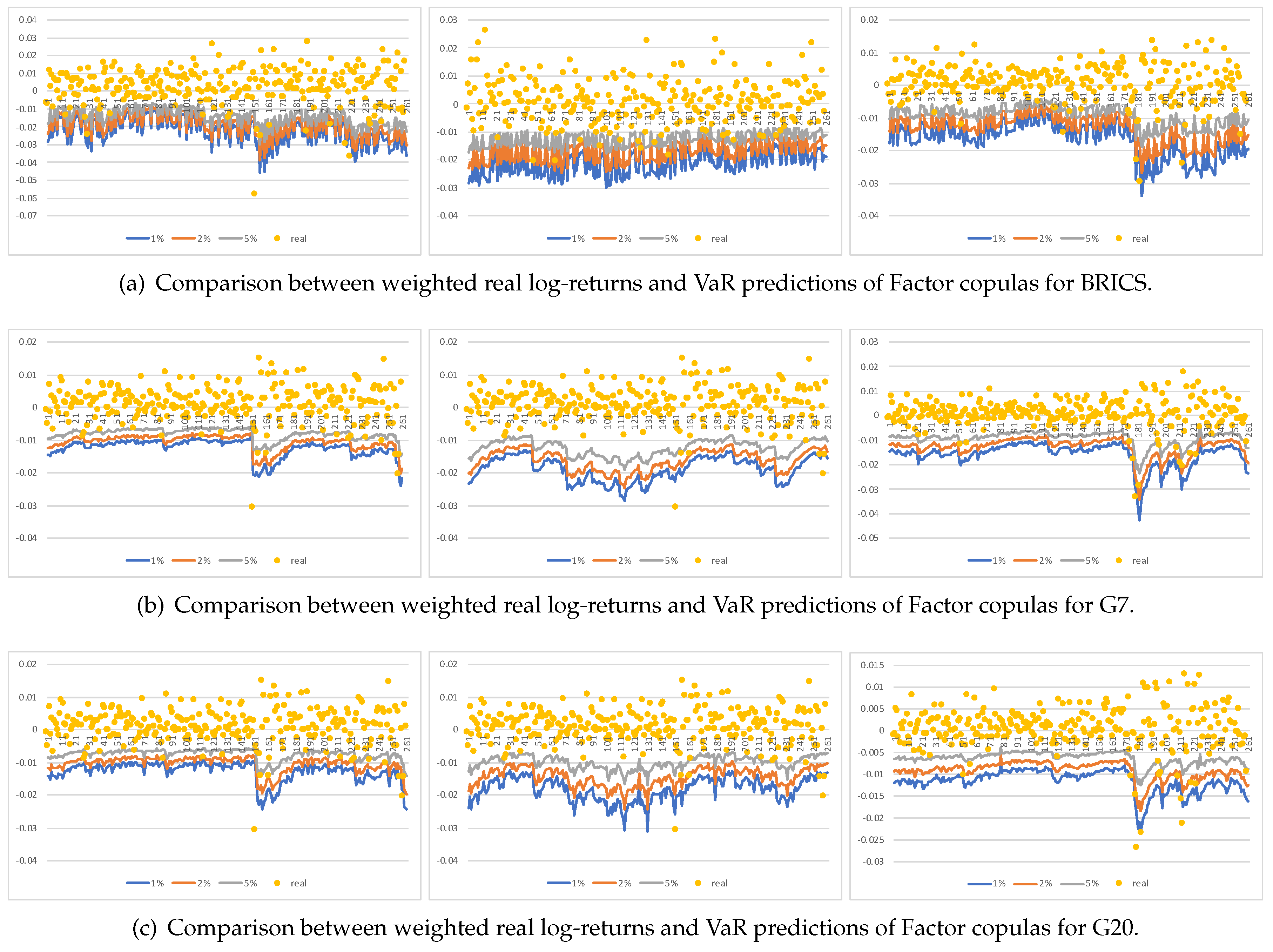
The various VaRs estimated from the Factor copulas are shown in Figure 2 with $\alpha$ = 0.01, 0.02, and 0.05, respectively. We analyzed some obvious violations in the three periods. For BRICS, in the pre-crisis period, at the 152th prediction, there was an extraordinary violation on 27 February 2007. On that day, the Shanghai composite index slumped 8.84%, which was the maximum daily drawdown in the past 10 years. On the same day, many stock indexes of G7 and G20 suffered huge losses, such as SPX (America), which dropped 3.53%, S&P/TSX (Canada) which dropped 2.72%, DAX (Germany) which dropped 2.96%, and UKX (England) which dropped 2.31%, so that day was named “Black Tuesday” in many countries. The Factor copula models captured the sharp downward trend and provided a potential risk alarm for G7 and G20. For the 151th prediction in the crisis period, which refers to 31 July 2012, SPX decreased by 4.33%, and for G7 and G20, especially for G20’s VaR prediction, there were significant downward trends, which also shows the risk to investors who own portfolios that include the SPX index. In the post-crisis period, the 180th and 211th predictions were severe violations, which refer to 28 February and 23 March 2018, respectively. Partially due to a slide in the price of oil, U.S. stocks sank again on 28 February and that February was the worst month for the market in past two years. Affected by the poor performance of U.S. stock markets, 16 of the rest of the 18 countries’ stock markets suffered a drop. Additionally, after U.S. President Donald Trump slapped China with annual tariffs, on 23 March 2018, markets witnessed a steep decline. Our results show that Factor copulas successfully indicated the risk. Noteworthy as well is that, even when the causes of the decline in two cases were not the same (oil price and policy change), Factor copulas still performed well.

4.3. Estimation of ES

In order to determine the best model for prediction, an intuitive method was applied to measure the accuracy of three methods by calculating the average distance square between the real log-returns and ESs corresponding to the violations of VaR:

$$\begin{array}{c}\hfill D=\sum _{i=1}^{261}\left[{({\overline{ES}}_i-R{t}_i)}^2{\mathbb{I}}_i\right]/\sum _{i=1}^{261}{\mathbb{I}}_i\end{array}$$

(16)

$${\mathbb{I}}_i=\left\{\begin{array}{cc}0\hfill & \mathrm{if}Va{R}_i<R_i,\hfill \\ 1\hfill & \mathrm{others}.\hfill \end{array}\right.$$

where ${\overline{ES}}_i$ is the i-th prediction of ES, and R${}_i$ is the real weighted log-return.

The results are shown in

Table 6. Results for the average distance between Estimate Shortfalls (ESs) and real log-returns.

Group	Period	Method	ES 1%	ES 2%	ES 5%
BRICS	pre	factor	1.939 × 10${}^{-4}$	1.450 × 10${}^{-4}$	1.159 × 10${}^{-4}$
		c-vine	2.532 × 10${}^{-4}$	1.756 × 10${}^{-4}$	1.089 × 10${}^{-4}$
	in	factor	7.478 × 10${}^{-6}$	6.572 × 10${}^{-6}$	5.406 × 10${}^{-6}$
		c-vine	1.115 × 10${}^{-8}$	1.257 × 10${}^{-6}$	5.259 × 10${}^{-6}$
		d-vine	5.874 × 10${}^{-9}$	1.182 × 10${}^{-6}$	4.894 × 10${}^{-6}$
	post	factor	9.084 × 10${}^{-6}$	7.530 × 10${}^{-6}$	1.207 × 10${}^{-5}$
		c-vine	1.547 × 10${}^{-5}$	1.734 × 10${}^{-5}$	2.814 × 10${}^{-5}$
		d-vine	1.577 × 10${}^{-5}$	1.742 × 10${}^{-5}$	2.850 × 10${}^{-5}$
G20	pre	factor	1.529 × 10${}^{-4}$	5.750 × 10${}^{-5}$	3.226 × 10${}^{-5}$
		c-vine	1.027 × 10${}^{-4}$	1.241 × 10${}^{-4}$	5.104 × 10${}^{-5}$
		d-vine	1.641 × 10${}^{-4}$	1.310 × 10${}^{-4}$	4.873 × 10${}^{-5}$

Bold indicates the smallest value of the calculation.

.

For BRICS, it is hard to determine which copula is the best for measuring the risk. For G7, only Factor copulas failed to reject the LR${}_{UC}$, LR${}_{IND}$ and LR${}_{CC}$ test, which shows the weak performance of Vine copulas in 7-dimensional data. As for G20, it was only in the pre-crisis period that the C-Vine copula performed a little bit better than the Factor copula, while in other cases, C-Vine and D-Vine copulas were overwhelmed by the Factor copula. It is clear to see that the Factor copula can provide a better prediction.

In order to compare the risk among BRICS, G7, and G20, the ES was adopted to represent the potential risk. Figure 3 shows ES estimation of three groups in three periods by the Factor copula model and all slumps in it appear the same time as Figure 3, which indicates that, for ES and VaR, they share the same reasons for steep fall. As for the figure for ES estimation result, there are three main findings.

Firstly, during the crisis period, potential risk was higher than in the pre-crisis and post-crisis periods, since there was a higher absolute value of ES and huge fluctuations throughout the crisis period. Additionally, because of successful remedial measures, including policy change and deleverage, the potential risk in the post-crisis period was less than in the pre-crisis period.

Secondly, in the pre-crisis period, in terms of both values and fluctuation, BRICS showed higher risk than the other two groups. In more than half of the days in the crisis and post-crisis periods, the absolute value of ES of BRICS was higher than in the other countries, and it had more fluctuation. Generally speaking, in all periods, BRICS countries contain more risk than G7 and G20, because it is more dangerous for the financial stability of banks and rate of return of investors to have frequent extreme fluctuations or sharp declines in a short time than over the long run. The reasons for the fluctuations and declines of BRICS may be immature policy, lax supervision, defective financial sectors, and so on. These drawbacks are common problems for emerging markets.

Thirdly, in the pre-crisis period, the curves of G7 and G20 are nearly overlapping, which indicates that G7 still dominates other countries in G20 group. Additionally, as time passed by, the gap between those two curves increased, and the risk for G20 was less than that of G7, since the strong economic performance of emerging markets like China and India and other developed countries which are not members of G7, like Australia and Korea, diversified the potential risk. Additionally, obviously, in the post-crisis period, the ES curve of G7 was below G20’s, which indicates the fact that G7 is more risky. It also means that other countries are playing more important roles in the global economy.

5. Conclusions

In this paper, for the purpose of risk measurement, combined with ARMA(1,1)-GJR-GARCH(1,1), two new kinds of copula were adopted to fit the data and to predict VaR and ES. In order to differentiate the risk among emerging markets, advanced economies, and the global economy, a comparison among the three groups was discussed. Several findings obtained from the Factor copula model indicate the effectiveness and practicality.

A comparison between Vine and Factor copulas is shown by both simulated data and real data, which reveals the unique advantages for the Factor copula model. Firstly, Factor copulas showed accuracy in their predictions of VaR and ES. Secondly, the stability of the predictions was proved. Thirdly, for high-dimensional data, Factor copulas tended to be better than Vine copulas, due to the overestimation of the risk of Vine copulas. Besides, for policymakers and investors, the dependence between latent variables and stock indexes obtained from Factor copulas models is consistent with common knowledge. Therefore it is recommended to adopt this method to measure the potential risk for stock markets. And the discussion of potential risk order of BRICS, G7, and G20 (BRICS was the highest and G20 was the lowest) suggests that for the purpose of diversification, the portfolio with G20 may be a good choice. Moreover, estimation results for pre-crisis period by Factor copula models implied strong correlations among most of the countries, which may be an early alarm for an upcoming financial crisis.

One-Factor copula models were adopted because of the limitation of the capacity of calculation. In this study, two or more factors were adopted at the first place, but for 19-dimensional data, the total calculation is huge. For further research, multiple-Factor copula models may be a better choice due to their modified code and higher calculation capacity computer. Besides, more detailed analysis, such as dependence between risk and oil prices or change-point analysis of the parameter of the copula, might provide more implications to policymakers.