Convergence Theorems for Common Solutions of Split Variational Inclusion and Systems of Equilibrium Problems

Abstract

In this paper, the split variational inclusion problem (SVIP) and the system of equilibrium problems (EP) are considered in Hilbert spaces. Inspired by the works of Byrne et al., López et al., Moudafi and Thukur, Sobumt and Plubtieng, Sitthithakerngkiet et al. and Eslamian and Fakhri, a new self-adaptive step size algorithm is proposed to find a common element of the solution set of the problems SVIP and EP. Convergence theorems are established under suitable conditions for the algorithm and application to the common solution of the fixed point problem, and the split convex optimization problem is considered. Finally, the performances and computational experiments are presented and a comparison with the related algorithms is provided to illustrate the efficiency and applicability of our new algorithms.

1. Introduction

Let $\varphi :C\times C\to \mathbb{R}$ be a bifunction, where C is a nonempty closed convex subset of a real Hilbert space H and $\mathbb{R}$ is the set of real numbers. The equilibrium problem (EP) for $\varphi$ is as follows:

$$\begin{array}{c}\hfill \mathrm{Find}\mathrm{a}\mathrm{point}{x}^{\ast }\in C\mathrm{such}\mathrm{that}\varphi (x^{\ast },y)\ge 0\mathrm{for}\mathrm{all}y\in C.\end{array}$$

(1)

The problem (EP) (1) represents a very suitable and common format for investigation and solution of various applied problems and involves many other general problems in nonlinear analysis, such as complementarity, fixed point, and variational inequality problems. A wide range of problems in finance, physics, network analysis, economics, and optimizations can be reduced to find the solution of the problem (1) (see, for instance, Blum and Oetti [1], Flam and Antipin [2], Moudafi [3], and Bnouhachem et al. [4]). Moreover, many authors have studied the methods and algorithms to approximate a solution of the problem (1), for instance, descent algorithms in Konnov and Ali [5], Konnov and Pinyagina [6], Charitha [7], and Lorenzo et al. [8]. For more details, refer to Ceng [9], Yao et al. [10,11,12], Qin et al. [13,14], Hung and Muu [15], Quoc et al. [16], Santos et al. [17], Thuy et al. [18], Rockafellar [19], Moudafi [20,21], Muu and Otelli [22], and Dong et al. [23].

On the other hand, many real-world inverse problems can be cast into the framework of the split inverse problem (SIP), which is formulated as follows:

$$\mathrm{Find}\mathrm{a}\mathrm{point}{x}^{\ast }\in X\mathrm{that}\mathrm{solves}\mathrm{the}\mathrm{problem}\mathrm{IP}1$$

and such that the point

$$y^{\ast }=A{x}^{\ast }\in Y\mathrm{solves}\mathrm{the}\mathrm{problem}\mathrm{IP}2,$$

where IP1 and IP2 are two inverse problems, X and Y are two vector spaces and $A:X\to Y$ is a linear operator.

Realistic problems can be represented by making different choices of the spaces X and Y (including the case $X=Y$) and by choosing appropriate inverse problems for the problems IP1 and IP2. In particular, the well-known split convex feasibility problem (SCFP) (Censor and Elfving [24]) is illustrated as follows:

$$\begin{array}{c}\hfill \mathrm{Find}\mathrm{a}\mathrm{point}{x}^{\ast }\mathrm{such}\mathrm{that}{x}^{\ast }\in C\mathrm{and}A{x}^{\ast }\in Q,\end{array}$$

(2)

where C and Q are nonempty closed and convex subsets of real Hilbert spaces $H_1$ and $H_2$, respectively, and A is a bounded and linear operator from $H_1$ to $H_2$. The problem SCFP (2) has received important attention due to its applications in signal processing, image reconstruction, with particular progress in intensity modulated radiation therapy, compressed sensing, approximating theory, and control theory (see, for example, [25,26,27,28,29,30,31,32] and the references therein).

Initiated by the problem SCFP, several split type problems have been investigated and studied, for example, split variational inequality problems, split common fixed point problems, and split null point problems. Especially, Moudafi [33] introduced the split monotone variational inclusion problem (SMVIP) for two operators $f_1:H_1\to H_1$ and $f_2:H_2\to H_2$ and multi-valued maximal monotone mappings $B_1$, $B_2$ as follows:

$$\begin{array}{c}\hfill \mathrm{Find}\mathrm{a}\mathrm{point}{x}^{\ast }\in H_1\mathrm{such}\mathrm{that}0\in f_1\left(x^{\ast }\right)+B_1\left(x^{\ast }\right)\end{array}$$

(3)

and

$$\begin{array}{c}\hfill y^{\ast }=A{x}^{\ast }\in H_2\mathrm{such}\mathrm{that}0\in f_2\left(y^{\ast }\right)+B_2\left(y^{\ast }\right).\end{array}$$

(4)

If $f_1=f_2=0$ in the problem SMVIPs (3) and (4), the problem SMVIP reduces to the following split variational inclusion problem (SVIP):

$$\begin{array}{c}\hfill \mathrm{Find}\mathrm{a}\mathrm{point}{x}^{\ast }\in H_1\mathrm{such}\mathrm{that}0\in B_1\left(x^{\ast }\right)\end{array}$$

(5)

and

$$\begin{array}{c}\hfill y^{\ast }=A{x}^{\ast }\in H_2\mathrm{such}\mathrm{that}0\in B_2\left(y^{\ast }\right).\end{array}$$

(6)

The problem SVIPs (5) and (6) constituted a pair of variational inclusion problems which have to be solved so that the image $y^{\ast }=A{x}^{\ast }$ under a given bounded linear operator A of the solution of the problem SVIP (5) in $H_1$ is the solution of the other SVIP (6) in another Hilbert space $H_2$. Indeed, one can see that $x^{\ast }\in B_1^{-1}\left(0\right)$ and $y^{\ast }=A{x}^{\ast }\in B_2^{-1}\left(0\right)$. The SVIPs (5) and (6) is at the core of modeling many inverse problems arising from phase retrieval and other real-world problems, for instance, in sensor networks in computerized tomography and data compression (see, for example, [34,35,36]).

In the process of studying equilibrium problems and split inverse problems, not only techniques and methods for solving the respective problems have been proposed (see, for example, CQ-algorithm in Byrne [37,38], relaxed CQ-algorithm in Yang [39] and Gibali et al. [40], self-adaptive algorithm in López et al. [41], Moudafi and Thukur [42], and Gibali [43]), but also the common solution of equilibrium problems, split inverse problems, and other problems have been considered in many works (see, for example, Plubtieng and Sombut [44] considered the common solution of equilibrium problems and nonspreading mappings; Sobumt and Plubtieng [45] studied a common solution of equilibrium problems and split feasibility problems in Hilbert spaces; Sitthithakerngkiet et al. [46] investigated a common solution of split monotone variational inclusion problems and fixed points problem of nonlinear operators; Eslamian and Fakhri [47] considered split equality monotone variational inclusion problems and fixed point problem of set-valued operators; Censor and Segal [48], Plubtieng and Sriprad [49] explored split common fixed point problems for directed operators). In particular, some applications to mathematical models for studying a common solution of convex optimizations and compressed sensing whose constraints can be presented as equilibrium problems and split variational inclusion problems, which stimulated our research on this kind of problem.

Motivated by the above works, we consider the following split variational inclusion problem and equilibrium problem:

Let $H_1$ and $H_2$ be real Hilbert spaces, $A:H_1\to H_2$ be a bounded linear operator. Let $B_1:H_1\to 2^{H_1}$ and $B_2:H_2\to 2^{H_2}$ be two set-valued mappings with nonempty values and $\varphi :C\times C\to \mathbb{R}$ be a bifunction, where C is nonempty closed convex subset of $H_1$.

The split monotone variational inclusion and equilibrium problem (SMVIEP) is as follows:

$$\begin{array}{c}\hfill \mathrm{Find}\mathrm{a}\mathrm{point}{x}^{\ast }\in \mathrm{EP}\left(\varphi \right)\cap B_1^{-1}\left(0\right)\end{array}$$

(7)

such that

$$\begin{array}{c}\hfill y^{\ast }=A{x}^{\ast }\in B_2^{-1}\left(0\right),\end{array}$$

(8)

where $\mathrm{EP}\left(\varphi \right)$ denotes the solution set of the problem EP.

Combined with techniques of Byrne et al., López et al., Moudafi and Thukur, Sitthithakerngkiet et al. as well as of Sobumt and Plubtieng and Eslamian and Fakhri, the purpose of this paper is to introduce a new iterative method which is called a new self-adaptive step size algorithm for solving the problem SMVIEPs (7) and (8) in Hilbert spaces.

The outline of the paper is as follows: In Section 2, we collect definitions and results which are needed for our further analysis. In Section 3, our new self-adaptive step size algorithms are introduced and analyzed, the weak and strong convergence theorems for the proposed algorithms are obtained, respectively, under suitable conditions. Moreover, as applications, the existence of a fixed point of a pseudo contractive mapping and a solution of the split convex optimization problem is considered in Section 4. Finally, the numerical examples and a comparison with some related algorithms are presented to illustrate the performances of our new algorithms.

2. Preliminaries

Now, we recall some concepts and results which are needed in the sequel.

Let H be a Hilbert space with the inner product $⟨·,·⟩$ and the induced norm $\parallel ·\parallel$ and I be the identity operator on H. Let $Fix\left(T\right)$ denote the fixed point set of an operator T if T has fixed point. The symbols $‘‘\to "$ and $‘‘\rightharpoonup "$ represent the strong and the weak convergence, respectively. For any sequence $\left\{x_n\right\}\subset H$, $w_w\left(x_n\right)$ denotes the weak w-limit set of $\left\{x_n\right\}$, that is,

$$\begin{array}{c}\hfill w_w\left(x_n\right):=\{x\in H:x_{n_j}\rightharpoonup x\mathrm{for}\mathrm{some}\mathrm{subsequence}\left\{n_j\right\}\mathrm{of}\left\{n\right\}\}.\end{array}$$

(9)

The following properties of the norm in a Hilbert space H are well known:

$$\begin{array}{ccc}\hfill {\parallel \alpha x+\beta y+\gamma z\parallel }^2& =& {\alpha \parallel x\parallel }^2+{\beta \parallel y\parallel }^2+\gamma {\parallel z\parallel }^2\hfill \\ & & {-\alpha \beta \parallel x-y\parallel }^2{-\beta \gamma \parallel y-z\parallel }^2-\gamma \alpha {\parallel x-z\parallel }^2\hfill \end{array}$$

(10)

for all $x,y,z\in H$ and $\alpha ,\beta ,\gamma \ge 0$. Moreover, the following inequality holds: for all $x,y\in H$,

$$\begin{array}{c}\hfill {\parallel x+y\parallel }^2\le {\parallel x\parallel }^2+2⟨y,x+y⟩\end{array}$$

(11)

Let C be a closed convex subset of H. For all $x\in H$, there exists a unique nearest point in C, denote $P_{C}x$, such that

$$\begin{array}{c}\hfill \parallel x-P_{C}x\parallel =min\{\parallel x-y\parallel :y\in C\}.\end{array}$$

(12)

The operator $P_C$ is called the metric projection of H onto C. Some properties of the operator $P_C$ are as follows: for all $x,y\in H$,

$$\begin{array}{c}\hfill ⟨x-y,P_{C}x-P_{C}y⟩\ge {\parallel P_{C}x-P_{C}y\parallel }^2\end{array}$$

(13)

and, for all $x\in H$ and $y\in C$,

$$\begin{array}{c}\hfill ⟨x-P_{C}x,y-P_{C}x⟩\le 0.\end{array}$$

(14)

Definition 1.

Let H be a real Hilbert space and D be a subset of H. For all $x,y\in D$, an operator $h:D\to H$ is said to be:

(1) 

firmly nonexpansive on D if

$$\begin{array}{c}\hfill ⟨h\left(x\right)-h\left(y\right),x-y⟩\ge {\parallel h\left(x\right)-h\left(y\right)\parallel }^2.\end{array}$$

(15)

(2) 

Lipschitz continuous with constant $\kappa >0$ on D if

$$\begin{array}{c}\hfill \parallel h\left(x\right)-h\left(y\right)\parallel \le \kappa \parallel x-y\parallel .\end{array}$$

(16)

(3) 

nonexpansive on D if

$$\begin{array}{c}\hfill \parallel h\left(x\right)-h\left(y\right)\parallel \le \parallel x-y\parallel .\end{array}$$

(17)

(4) 

hemicontinuous if it is continuous along each line segment in D.

(5) 

averaged if there exist a nonexpansive operator $T:D\to H$ and a number $c\in (0,1)$ such that

$$\begin{array}{c}\hfill h=(1-c)I+cT.\end{array}$$

(18)

Remark 1.

The following can be easily obtained:

(1) 

An operator h is firmly nonexpansive if and only if $I-h$ is firmly nonexpansive (see [50], Lemma 2.3), then h is nonexpansive.

(2) 

If $h_1$ and $h_2$ are averaged, then their composition $S=h_1\circ h_2$ is averaged (see [50], Lemma 2.2).

Definition 2.

Let H be a real Hilbert space and $\lambda >0$. The operator $B:H\to 2^H$ is said to be:

(1) 

monotone if, for all $u\in B\left(x\right)$ and $v\in B\left(y\right)$,

$$\begin{array}{c}\hfill ⟨u-v,x-y⟩\ge 0.\end{array}$$

(19)

(2) 

maximal monotone if the graph $Graph\left(B\right)$ of B,

$$\begin{array}{c}\hfill Graph\left(B\right):=\left\{\right(x,u)\in H\times H:u\in B(x\left)\right\},\end{array}$$

(20)

is not properly contained in the graph of any other monotone mapping.

(3) 

The resolvent of B with parameter $\lambda >0$ is denoted by

$$\begin{array}{c}\hfill J_{\lambda }^B:={(I+\lambda B)}^{-1},\end{array}$$

(21)

where I is the identity operator.

Remark 2.

For any $\lambda >0$, the following hold:

(1) 

B is maximal monotone if and only if $J_{\lambda }^B$ is single-valued, firmly nonexpansive, and $dom\left(J_{\lambda }^B\right)=H$, where $dom\left(B\right):=\{x\in H:B(x)\ne \varnothing \}$.

(2) 

$x^{\ast }\in B^{-1}\left(0\right)$ if and only if $x^{\ast }=J_{\lambda }^B{x}^{\ast }$.

(3) 

The solution set Ω of the problem SVIPs (5) and (6) is equivalent to the following:

$$\begin{array}{c}\hfill \mathit{Find}a\mathit{point}{x}^{\ast }\in H_1\mathit{with}{x}^{\ast }=J_{\lambda }^{B_1}{x}^{\ast }\mathit{such}\mathit{that}{y}^{\ast }=A{x}^{\ast }\in H_2\mathit{and}{y}^{\ast }=J_{\lambda }^{B_2}{y}^{\ast }.\end{array}$$

(22)

(4) 

For some more results, refer to [33,36,51].

Assume that an equilibrium bifunction $\varphi :C\times C\to \mathbb{R}$ satisfies the following conditions:

(A1)

$\varphi (x,x)=0$ for all $x\in C$;

(A2)

$\varphi (x,y)+\varphi (y,x)\le 0$ for all $x,y\in C$;

(A3)

For all $x,y,z\in C$, ${lim}_{t\to 0}\varphi (tz+(1-t)x,y)\le \varphi (x,y)$ for all $x\in C$;

(A4)

For all $x\in C$, $y\to \varphi (x,y)$ is convex and lower semi-continuous.

Lemma 1.

(see [2]) Let C be a nonempty closed convex subset of a Hilbert space H and suppose that $\varphi :C\times C\to \mathbb{R}$ satisfies the conditions $\left(\mathbf{A}\mathbf{1}\right)$–$\left(\mathbf{A}\mathbf{4}\right)$. For all $r>0$ and $x\in H$, define a mapping $T_r:H\to C$ by

$$\begin{array}{c}\hfill T_r\left(x\right)=\{z\in C:\varphi (z,y)+\frac{1}{r}⟨y-z,z-x⟩\ge 0\}.\end{array}$$

(23)

Then the following hold:

(1) 

$T_r$ is nonempty single-valued.

(2) 

$T_r$ is firmly nonexpansive, that is, for all $x,y\in C$,

$$\begin{array}{c}\hfill ⟨T_{r}x-T_{r}y,x-y⟩\ge {\parallel T_{r}x-T_{r}y\parallel }^2\end{array}$$

and, further, $T_r$ is nonexpansive.

(3) 

$\mathrm{EP}\left(\varphi \right)=Fix\left(T_r\right)$ is closed and convex.

Lemma 2.

(see [26,52]) Assume that $\left\{a_n\right\}$ is a sequence of nonnegative real numbers such that, for each $n\ge 0$,

$$\begin{array}{c}\hfill a_{n+1}\le (1-{\theta }_n)a_n+{\delta }_n,\end{array}$$

(24)

where $\left\{{\theta }_n\right\}$ is a sequence in $(0,1)$ and $\left\{{\delta }_n\right\}$ is a sequence such that

(a) 

${lim}_{n\to \infty }{\theta }_n=0$ and ${\mathsf{\Sigma }}_{n=1}^{\infty }{\theta }_n=\infty$;

(b) 

$lim{sup}_{n\to \infty }\frac{{\delta }_n}{{\theta }_n}\le 0$ or ${\mathsf{\Sigma }}_{n=1}^{\infty }\left|{\delta }_n\right|<\infty$.

Then the limit of the sequence $\left\{a_n\right\}$ exists and ${lim}_{n\to \infty }{a}_n=0$.

Lemma 3.

(see [53]) Assume that $\left\{a_n\right\}$ and $\left\{{\delta }_n\right\}$ are the sequences of nonnegative numbers such that, for each $n\ge 0$,

$$\begin{array}{c}\hfill a_{n+1}\le a_n+{\delta }_n.\end{array}$$

(25)

If $lim{sup}_{n\to \infty }{\delta }_n\le \infty$ and $\left\{a_n\right\}$ has a subsequence converging to zero, then ${lim}_{n\to \infty }{a}_n=0$.

Lemma 4.

(see [52]) Let $\left\{{\mathsf{\Gamma }}_n\right\}$ be a sequence of real numbers that does not decrease at infinity, in the sense that there exists a subsequence $\left\{{\mathsf{\Gamma }}_{n_j}\right\}$ of $\left\{{\mathsf{\Gamma }}_n\right\}$ such that ${\mathsf{\Gamma }}_{n_j}<{\mathsf{\Gamma }}_{n_{j+1}}$ for each $j\ge 0$. Also, consider the sequence ${\left\{\sigma \left(n\right)\right\}}_{n\ge n_0}$ of integers defined by

$$\begin{array}{c}\hfill \sigma \left(n\right)=max\{k\le n:{\mathsf{\Gamma }}_k\le {\mathsf{\Gamma }}_{k+1}\}.\end{array}$$

(26)

Then ${\left\{\sigma \left(n\right)\right\}}_{n\ge n_0}$ is a nondecreasing sequence satisfying ${lim}_{n\to \infty }\sigma \left(n\right)=\infty$ and, for each $n\ge n_0$,

$$\begin{array}{c}\hfill max\{{\mathsf{\Gamma }}_{\sigma \left(n\right)},{\mathsf{\Gamma }}_n\}\le {\mathsf{\Gamma }}_{\sigma \left(n\right)+1}.\end{array}$$

(27)

Lemma 5.

(see [54]) Let C be a nonempty closed convex subset of a real Hilbert space H. If $T:C\to C$ is nonexpansive and $Fix\left(T\right)\ne \varnothing$, then the mapping $I-T$ is demiclosed at 0, that is, if $\left\{x_n\right\}$ is a sequence in C converges weakly to $x^{\ast }$ and $\parallel x_n-T{x}_n\parallel \to 0$, then $x^{\ast }=T{x}^{\ast }$.

3. The Main Results

In this section, we introduce our algorithms and state our main results.

Throughout this paper, we always assume that $H_1$ and $H_2$ are Hilbert spaces, C is a nonempty closed convex subset of $H_1$, the bifunction $\varphi :C\times C\to \mathbb{R}$ satisfies the conditions $\left(\mathbf{A}\mathbf{1}\right)$–$\left(\mathbf{A}\mathbf{4}\right)$, $A:H_1\to H_2$ is a bounded linear operator, $A^{\ast }$ denotes the conjugate transpose of A (in finite dimensional spaces, $A^{\ast }=A^T$). Let $B_1:H_1\to 2^{H_1}$ and $B_2:H_2\to 2^{H_2}$ be two maximal monotone operators.

Now, we define the functions by

$$\begin{array}{c}\hfill f\left(x\right)=\frac{1}{2}\parallel (I-J_{\lambda }^{B_2}){Ax\parallel }^2,g\left(x\right)=\frac{1}{2}{\parallel (I-J_{\lambda }^{B_1})x\parallel }^2,\end{array}$$

(28)

and

$$\begin{array}{c}\hfill F\left(x\right)=A^{\ast }(I-J_{\lambda }^{B_2})Ax,G\left(x\right)=(I-J_{\lambda }^{B_1})x,\end{array}$$

(29)

where $J_{\lambda }^B={(I+\lambda B)}^{-1}$ for any $\lambda >0$.

From Aubin [55], one can see that f and g are weakly lower semi-continuous and convex differentiable. Moreover, it is known that the functions F and G are Lipschitz continuous according to Beryne et al. [36]. Denote the solution of the problem SVIPs (5) and (6) by

$$\begin{array}{c}\hfill \mathsf{\Omega }=\{x^{\ast }\in H_1:0\in B_1\left(x^{\ast }\right),0\in B_2\left(A{x}^{\ast }\right)\}.\end{array}$$

(30)

3.1. Iterative Algorithms

Now, we introduce the following 3 algorithms for our main results:

Algorithm 1.Choose a positive sequence $\left\{{\rho }_n\right\}$ satisfying $\epsilon <{\rho }_n<4-\epsilon$ for some $\epsilon >0$ small enough. Select arbitrary starting point $x_0$, set $n=0$ and let $r>0$, $\lambda >0$.

Iterative Step: For any iterate $x_n$ for each $n\ge 0$, compute $$\varphi (z_n,y)+\frac{1}{r}⟨y-z_n,z_n-x_n⟩\ge 0,$$ $$y_n={\beta }_n{x}_n+(1-{\beta }_n)z_n,$$ $$\begin{array}{c}\hfill {\gamma }_n=\left\{\begin{array}{cc}\frac{{\rho }_n(f\left(y_n\right)+g\left(y_n\right))}{\parallel F\left(y_n\right){\parallel }^2+{\parallel G\left(y_n\right)\parallel }^2},\hfill & \parallel F\left(y_n\right){\parallel }^2+{\parallel G\left(y_n\right)\parallel }^2\ne 0,\hfill \\ 0,\hfill & otherwise,\hfill \end{array}\right.\end{array}$$ and calculate the next iterate as $$\begin{array}{c}\hfill x_{n+1}={\alpha }_n{x}_n+(1-{\alpha }_n)J_{\lambda }^{B_1}(I-{\gamma }_n{A}^{\ast }(I-J_{\lambda }^{B_2})A)y_n,\end{array}$$ (31) where $\left\{{\alpha }_n\right\}$ and $\left\{{\beta }_n\right\}$ are the sequences in $(0,1)$.  Stop Criterion: If $x_{n+1}=x_n=y_n$, then stop. Otherwise, set $n:=n+1$ and return to Iterative Step.

Algorithm 2.Choose a positive sequence $\left\{{\rho }_n\right\}$ satisfying $\epsilon <{\rho }_n<4-\epsilon$ (for some $\epsilon >0$ small enough). Select arbitrary starting point $x_0$, set $n=0$ and let $r>0$, $\lambda >0$.

Iterative Step: For any iterate $x_n$ for each $n\ge 0$, compute $$\varphi (z_n,y)+\frac{1}{r}⟨y-z_n,z_n-x_n⟩\ge 0,$$ $$y_n={\beta }_n{x}_n+(1-{\beta }_n)z_n,$$ $$\begin{array}{c}\hfill {\gamma }_n=\left\{\begin{array}{cc}\frac{{\rho }_n(f\left(y_n\right)+g\left(y_n\right))}{\parallel F\left(y_n\right){\parallel }^2+{\parallel G\left(y_n\right)\parallel }^2},\hfill & \parallel F\left(y_n\right){\parallel }^2+{\parallel G\left(y_n\right)\parallel }^2\ne 0,\hfill \\ 0,\hfill & otherwise,\hfill \end{array}\right.\end{array}$$ and calculate the next iterate as $$\begin{array}{c}\hfill x_{n+1}={\alpha }_n{x}_0+(1-{\alpha }_n)J_{\lambda }^{B_1}(I-{\gamma }_n{A}^{\ast }(I-J_{\lambda }^{B_2})A)y_n,\end{array}$$ (32) where $\left\{{\alpha }_n\right\}$ and $\left\{{\beta }_n\right\}$ are the sequences in $(0,1)$.  Stop Criterion: If $x_{n+1}=x_n=y_n$, then stop. Otherwise, set $n:=n+1$ and return to Iterative Step.

Algorithm 3.Choose a positive sequence $\left\{{\rho }_n\right\}$ satisfying $\epsilon <{\rho }_n<4-\epsilon$ (for some $\epsilon >0$ small enough). Select arbitrary starting point $x_0$, set $n=0$ and let $r>0$, $\lambda >0$.

Iterative Step: For any iterate $x_n$ for each $n\ge 0$, compute $$\varphi (z_n,y)+\frac{1}{r}⟨y-z_n,z_n-x_n⟩\ge 0,$$ $$y_n={\beta }_n{x}_n+(1-{\beta }_n)z_n,$$ $$\begin{array}{c}\hfill {\gamma }_n=\left\{\begin{array}{cc}\frac{{\rho }_n(f\left(y_n\right)+g\left(y_n\right))}{\parallel F\left(y_n\right){\parallel }^2+{\parallel G\left(y_n\right)\parallel }^2},\hfill & \parallel F\left(y_n\right){\parallel }^2+{\parallel G\left(y_n\right)\parallel }^2\ne 0,\hfill \\ 0,\hfill & otherwise,\hfill \end{array}\right.\end{array}$$ and calculate the next iterate as $$\begin{array}{c}\hfill x_{n+1}=(1-{\alpha }_n-{\tau }_n)x_n+{\alpha }_n{J}_{\lambda }^{B_1}(I-{\gamma }_n{A}^{\ast }(I-J_{\lambda }^{B_2})A)y_n,\end{array}$$ (33) where $\left\{{\alpha }_n\right\}$, $\left\{{\beta }_n\right\}$ and ${\tau }_n$ are the sequences in $(0,1)$ with ${\alpha }_n+{\tau }_n\le 1$.  Stop Criterion: If $x_{n+1}=x_n=y_n$, then stop. Otherwise, set $n:=n+1$ and return to Iterative Step.

3.2. Weak Convergence Analysis for Algorithm 1

First, we give one lemma for our main result.

Lemma 6.

Suppose that $\mathrm{EP}\left(\varphi \right)\cap \mathsf{\Omega }\ne \varnothing$. If $x_{n+1}=y_n=x_n$ in Algorithm 1, then $x_n\in \mathrm{EP}\left(\varphi \right)\cap \mathsf{\Omega }$.

Proof. 

Denote $T_r\left(x_n\right)=\{z_n\in C,\varphi (z_n,y)+\frac{1}{r}⟨y-z_n,z_n-x_n⟩\ge 0\}$. Then we can see $z_n=T_r{x}_n$.

If $x_n=y_n$, then it follows from the construction of $y_n$ that $x_n=z_n$ and hence $x_n\in Fix\left(T_r\right)$, that is, $x_n\in \mathrm{EP}\left(\varphi \right)$ from Lemma 1.

On the other hand, the operator $J_{\lambda }^{B_1}$ and $I-{\gamma }_n{A}^{\ast }(I-J_{\lambda }^{B_2})A$ are averaged from Remark 1. Since $\mathsf{\Omega }\ne \varnothing$, it follows from Lemma 2.1 of [51], with the averaged operators $J_{\lambda }^{B_1}$ and $I-{\gamma }_n{A}^{\ast }(I-J_{\lambda }^{B_2})A$, that

$$\begin{array}{ccc}\hfill Fix\left(J_{\lambda }^{B_1}\right)\bigcap Fix(I-{\gamma }_n{A}^{\ast }(I-J_{\lambda }^{B_2})A)& =& Fix\left(J_{\lambda }^{B_1}(I-{\gamma }_n{A}^{\ast }(I-J_{\lambda }^{B_2})A)\right)\hfill \\ & =& Fix\left((I-{\gamma }_n{A}^{\ast }(I-J_{\lambda }^{B_2})A)J_{\lambda }^{B_1}\right).\hfill \end{array}$$

(34)

If $x_{n+1}=y_n=x_n$, then we can see $x_n=J_{\lambda }^{B_1}(I-{\gamma }_n{A}^{\ast }(I-J_{\lambda }^{B_2})A)x_n$ from the recursion (31) and hence $x_n\in Fix\left(J_{\lambda }^{B_1}\right)$ and $x_n\in Fix(I-{\gamma }_n{A}^{\ast }(I-J_{\lambda }^{B_2})A)$, that is, $x_n\in B_1^{-1}\left(0\right)$ and

$$\begin{array}{c}\hfill (I-{\gamma }_n{A}^{\ast }(I-J_{\lambda }^{B_2})A)x_n=x_n⟹A^{\ast }(I-J_{\lambda }^{B_2})A{x}_n=0.\end{array}$$

(35)

It can be written as $J_{\lambda }^{B_2}A{x}_n=A{x}_n+w$, where $A^{\ast }w=0$. Without loss generality, if we take $z\in \mathsf{\Omega }$, then $J_{\lambda }^{B_2}Az=Az$ and $J_{\lambda }^{B_2}A{x}_n-J_{\lambda }^{B_2}Az=A{x}_n+w-Az$ and so

$$\begin{array}{ccc}\hfill \parallel A{x}_n{-Az\parallel }^2& \ge & \parallel J_{\lambda }^{B_2}\left(A{x}_n\right)-J_{\lambda }^{B_2}\left(Az\right){\parallel }^2\hfill \\ \hfill & =& \parallel A{x}_n{+w-Az\parallel }^2\hfill \\ \hfill & =& \parallel A{x}_n{-Az\parallel }^2+2⟨A{x}_n-Az,w⟩+{\parallel w\parallel }^2\hfill \\ \hfill & =& \parallel A{x}_n{-Az\parallel }^2+2⟨x_n-z,A^{\ast }w⟩+{\parallel w\parallel }^2\hfill \\ & =& \parallel A{x}_n{-Az\parallel }^2+{\parallel w\parallel }^2,\hfill \end{array}$$

(36)

which means that $\parallel w\parallel =0$ and so $J_{\lambda }^{B_2}A{x}_n=A{x}_n$, that is, $A{x}_n\in B_2^{-1}\left(0\right)$. Hence $x_n\in \mathsf{\Omega }$ and, furthermore, $x_n\in \mathrm{EP}\left(\varphi \right)\bigcap \mathsf{\Omega }$. This completes the proof. □

Theorem 1.

Let $H_1$, $H_2$ be two real Hilbert spaces and $A:H_1\to H_2$ be a bounded linear operator. Let ϕ be a bifunction satisfying the conditions $\left(\mathbf{A}\mathbf{1}\right)$–$\left(\mathbf{A}\mathbf{4}\right)$. Assume that $B_1:H_1\to 2^{H_1}$ and $B_2:H_2\to 2^{H_2}$ are maximal monotone mappings with $\mathrm{EP}\left(\varphi \right)\bigcap \mathsf{\Omega }\ne \varnothing$. Then the sequence $\left\{x_n\right\}$ generated by Algorithm 1 converges weakly to an element of $\mathrm{EP}\left(\varphi \right)\bigcap \mathsf{\Omega }$, where the parameters $\left\{{\alpha }_n\right\}$, $\left\{{\beta }_n\right\}$ are in $(0,1)$ and satisfy the following conditions:

$$\underset{n\to \infty }{lim}{\alpha }_n=0,{\mathsf{\Sigma }}_{n=1}^{\infty }|{\beta }_n-{\beta }_{n-1}|<\infty ,{\mathsf{\Sigma }}_{n=1}^{\infty }|{\alpha }_n-{\alpha }_{n-1}|<\infty .$$

Proof. 

Denote $T_n=I-{\gamma }_n{A}^{\ast }(I-J_{\lambda }^{B_2})A$. Since $J_{\lambda }^{B_2}$ is firmly nonexpansive according to Remark 2, $T_n$ is averaged from (1), (2) of Remark 1 and $J_{\lambda }^{B_1}(I-{\gamma }_n{A}^{\ast }(I-J_{\lambda }^{B_2})A)$ is averaged and nonexpansive.

First, we show that the sequences $\left\{x_n\right\}$ and $\left\{y_n\right\}$ are bounded. Since $\mathrm{EP}\left(\varphi \right)\bigcap \mathsf{\Omega }\ne \varnothing$, we take $z\in \mathrm{EP}\left(\varphi \right)\bigcap \mathsf{\Omega }$ and then $z=T_r\left(z\right)$, $z=J_{\lambda }^{B_1}z$ and $Az=J_{\lambda }^{B_2}Az$. At the same time, it follows that $z_n=T_r{x}_n$ and $T_r$ is nonexpansive according to Lemma 1 and so

$$\begin{array}{ccc}\hfill \parallel y_n-z\parallel & \le & {\beta }_n\parallel x_n-z\parallel +(1-{\beta }_n)\parallel z_n-z\parallel \hfill \\ & \le & \parallel x_n-z\parallel \hfill \end{array}$$

(37)

and

$$\begin{array}{ccc}\hfill \parallel x_{n+1}-z\parallel & =& \parallel {\alpha }_n{x}_n+(1-{\alpha }_n)J_{\lambda }^{B_1}(I-{\gamma }_n{A}^{\ast }(I-J_{\lambda }^{B_2})A)y_n-z\parallel \hfill \\ \hfill & \le & {\alpha }_n\parallel x_n-z\parallel +(1-{\alpha }_n)\parallel y_n-z\parallel \hfill \\ & \le & \parallel x_n-z\parallel ,\hfill \end{array}$$

(38)

which means that the sequence $\left\{x_n\right\}$ is bounded and so are $\left\{y_n\right\}$, $\left\{z_n\right\}$ and $\left\{u_n\right\}$, where $z_n=T_r{x}_n$ and $u_n=T_n{y}_n$.

Next, we show $\parallel x_{n+1}-x_n\parallel \to 0.$ Since $z_n=T_r{x}_n$, we have $z_{n-1}=T_r{x}_{n-1}$ and, for all $y\in C$,

$$\begin{array}{c}\hfill \varphi (z_n,y)+\frac{1}{r}⟨y-z_n,z_n-x_n⟩\ge 0\end{array}$$

(39)

and

$$\begin{array}{c}\hfill \varphi (z_{n-1},y)+\frac{1}{r}⟨y-z_{n-1},z_{n-1}-x_{n-1}⟩\ge 0.\end{array}$$

(40)

Putting $y=z_{n-1}$ in (39) and $y=z_n$ in (40), we have

$$\begin{array}{c}\hfill \varphi (z_n,z_{n-1})+\frac{1}{r}⟨z_{n-1}-z_n,z_n-x_n⟩\ge 0\end{array}$$

(41)

and

$$\begin{array}{c}\hfill \varphi (z_{n-1},z_n)+\frac{1}{r}⟨z_n-z_{n-1},z_{n-1}-x_{n-1}⟩\ge 0.\end{array}$$

(42)

Adding the inequalities (41) and (42), since $\varphi$ is monotone from $\left(\mathbf{A}\mathbf{2}\right)$, we have

$$\begin{array}{c}\hfill \varphi (z_n,z_{n-1})+\varphi (z_{n-1},z_n)\le 0\Rightarrow ⟨z_n-z_{n-1},z_{n-1}-x_{n-1}-(z_n-x_n)⟩\ge 0,\end{array}$$

(43)

which implies that

$$\begin{array}{c}\hfill ⟨z_n-z_{n-1},z_{n-1}-z_n⟩+⟨z_n-z_{n-1},x_n-x_{n-1}⟩\ge 0,\end{array}$$

(44)

that is,

$$⟨z_n-z_{n-1},x_n-x_{n-1}⟩\ge {\parallel z_n-z_{n-1}\parallel }^2.$$

Furthermore, we have $\parallel z_n-z_{n-1}\parallel \le \parallel x_n-x_{n-1}\parallel$. According to the definition of the iterative sequence $\left\{y_n\right\}$, we have

$$\begin{array}{ccc}\hfill \parallel y_n-y_{n-1}\parallel & =& \parallel {\beta }_n{x}_n+(1-{\beta }_n)z_n-{\beta }_{n-1}{x}_{n-1}+(1-{\beta }_{n-1})z_{n-1}\parallel \hfill \\ \hfill & =& \parallel {\beta }_n(x_n-x_{n-1})+(1-{\beta }_n)(z_n-z_{n-1})+({\beta }_n-{\beta }_{n-1})(x_{n-1}-z_{n-1})\parallel \hfill \\ \hfill & \le & {\beta }_n\parallel x_n-x_{n-1}\parallel +(1-{\beta }_n)\parallel z_n-z_{n-1}\parallel +|{\beta }_n-{\beta }_{n-1}\left|\right\{\parallel x_{n-1}\parallel +\parallel z_{n-1}\parallel \}\hfill \\ & \le & \parallel x_n-x_{n-1}\parallel +|{\beta }_n-{\beta }_{n-1}\left|\right\{\parallel x_{n-1}\parallel +\parallel z_{n-1}\parallel \}\hfill \end{array}$$

(45)

and, since $u_n=T_n{y}_n$, we have

$$\begin{array}{ccc}\hfill \parallel u_n-u_{n-1}\parallel & =& \parallel y_n-{\gamma }_{n}F\left(y_n\right)-y_{n-1}+{\gamma }_{n-1}F\left(y_{n-1}\right)\parallel \hfill \\ & =& \parallel y_n-y_{n-1}\parallel +{\gamma }_n\parallel F\left(y_n\right)\parallel +{\gamma }_{n-1}\parallel F\left(y_{n-1}\right)\parallel \hfill \\ & \le & \parallel x_n-x_{n-1}\parallel +|{\beta }_n-{\beta }_{n-1}\left|\right\{\parallel x_{n-1}\parallel +\parallel z_{n-1}\parallel \}\hfill \\ & & +{\gamma }_n\parallel F\left(y_n\right)\parallel +{\gamma }_{n-1}\parallel F\left(y_{n-1}\right)\parallel .\hfill \end{array}$$

(46)

On the other hand, we have

$$\begin{array}{ccc}\hfill ⟨F\left(y_n\right),y_n-z⟩& =& ⟨A^{\ast }(I-J_{\lambda }^{B_2})A{y}_n,y_n-z⟩\hfill \\ \hfill & =& ⟨(I-J_{\lambda }^{B_2})A{y}_n-(I-J_{\lambda }^{B_2})Az,A{y}_n-Az⟩\hfill \\ \hfill & \ge & \parallel (I-J_{\lambda }^{B_2})A{y}_n{\parallel }^2\hfill \\ & =& 2f\left(y_n\right).\hfill \end{array}$$

(47)

Since $J_{\lambda }^{B_1}$ is nonexpansive, we have

$$\begin{array}{ccc}\hfill \parallel x_{n+1}{-z\parallel }^2& =& \parallel {\alpha }_n(x_n-z)+(1-{\alpha }_n)(J_{\lambda }^{B_1}(I-{\gamma }_n{A}^{\ast }(I-J_{\lambda }^{B_2})A)y_n-z){\parallel }^2\hfill \\ \hfill & \le & {\alpha }_n\parallel x_n{-z\parallel }^2+(1-{\alpha }_n)[\parallel y_n{-z\parallel }^2+{\gamma }_n^2\parallel F\left(y_n\right){\parallel }^2-2{\gamma }_n⟨F\left(y_n\right),y_n-z⟩]\hfill \\ \hfill & \le & {\alpha }_n\parallel x_n{-z\parallel }^2+(1-{\alpha }_n)[\parallel y_n{-z\parallel }^2+{\gamma }_n^2\parallel F\left(y_n\right){\parallel }^2-4{\gamma }_{n}f\left(y_n\right)]\hfill \\ & \le & \parallel x_n{-z\parallel }^2-{\rho }_n\left(\frac{4f\left(y_n\right)}{f\left(y_n\right)+g\left(y_n\right)}-{\rho }_n\right)\frac{{(f\left(y_n\right)+g\left(y_n\right))}^2}{\parallel F\left(y_n\right){\parallel }^2+{\parallel G\left(y_n\right)\parallel }^2}.\hfill \end{array}$$

(48)

For any $\epsilon >0$ small enough, the sequence $\left\{x_n\right\}$ is Fejer monotone with respect to $\mathrm{EP}\left(\varphi \right)\cap \mathsf{\Omega }$, which ensures the existence of the limit of $\{\parallel x_n-z\parallel \}$ and so we can denote $l\left(z\right)={lim}_{n\to \infty }\parallel x_n-z\parallel$. Thus it follows from (48) that

$$\begin{array}{c}\hfill {\rho }_n\left(\frac{4f\left(y_n\right)}{f\left(y_n\right)+g\left(y_n\right)}-{\rho }_n\right)\frac{{(h\left(y_n\right)+g\left(y_n\right))}^2}{\parallel F\left(y_n\right){\parallel }^2+{\parallel G\left(y_n\right)\parallel }^2}\le \parallel x_n{-z\parallel }^2-{\parallel x_{n+1}-z\parallel }^2\to 0\end{array}$$

(49)

since F and G are Lipschitz continuous from Byrne [36] and so $F\left(y_n\right)$ and $G\left(y_n\right)$ are bounded.

In addition, it also follows (48) that

$$\begin{array}{c}\hfill {\mathsf{\Sigma }}_{n=1}^{\infty }\frac{{(f\left(y_n\right)+g\left(y_n\right))}^2}{\parallel F\left(y_n\right){\parallel }^2+{\parallel G\left(y_n\right)\parallel }^2}<\infty ,\end{array}$$

(50)

which means that

$$\begin{array}{c}\hfill {\mathsf{\Sigma }}_{n=1}^{\infty }{\gamma }_n<\infty \end{array}$$

(51)

and hence it follows that $f\left(y_n\right)\to 0$ and $g\left(y_n\right)\to 0$ if and only if $f\left(y_n\right)+g\left(y_n\right)\to 0$ as $n\to \infty$.

Thus it follows from the above inequalities that

$$\begin{array}{ccc}\hfill \parallel x_{n+1}-x_n\parallel & \le & {\alpha }_n\parallel x_n-x_{n-1}\parallel +(1-{\alpha }_n)\parallel u_n-u_{n-1}\parallel +|{\alpha }_n-{\alpha }_{n-1}|\parallel x_{n-1}-u_{n-1}\parallel \hfill \\ \hfill & \le & {\alpha }_n\parallel x_n-x_{n-1}\parallel +(1-{\alpha }_n)(\parallel x_n-x_{n-1}\parallel +{\theta }_n)+|{\alpha }_n-{\alpha }_{n-1}|\parallel x_{n-1}-u_{n-1}\parallel \hfill \\ & \le & \parallel x_n-x_{n-1}\parallel +(1-{\alpha }_n){\theta }_n+|{\alpha }_n-{\alpha }_{n-1}|\parallel x_{n-1}-u_{n-1}\parallel ,\hfill \end{array}$$

(52)

where ${\theta }_n=|{\beta }_n-{\beta }_{n-1}\left|\right\{\parallel x_{n-1}\parallel +\parallel z_{n-1}\parallel \}+{\gamma }_n\parallel F\left(y_n\right)\parallel +{\gamma }_{n-1}\parallel F\left(y_{n-1}\right)\parallel$ and ${\mathsf{\Sigma }}_{n=1}^{\infty }{\theta }_n<\infty$. Note that it follows from the conditions of ${\alpha }_n$ and ${\beta }_n$, combining the formula (51), that the limit of $\parallel x_{n+1}-x_n\parallel$ exists from Lemma 3. Since the limit of $\parallel x_n-z\parallel$ exists, there exists a subsequence $\{x_{nk}-z\}$ of the sequence $\{x_n-z\}$ converges to a point and $x_{nk+1}-x_{nk}\to 0$. Thus it follows that $\parallel x_{n+1}-x_n\parallel \to 0$ from Lemma 3. Further, $\parallel z_n-x_n\parallel \to 0$ because of $x_{n+1}-x_n=(1-{\alpha }_n)(1-{\beta }_n)(z_n-x_n)$ and $\parallel x_n-y_n\parallel =(1-{\beta }_n)\parallel x_n-z_n\parallel \to 0$.

Next, we show $x^{\ast }\in \mathrm{EP}\left(\varphi \right)\bigcap \mathsf{\Omega }$, where $x^{\ast }$ is a weak cluster of the sequence $\left\{x_n\right\}$. Note that $\left\{x_n\right\}$ is bounded and so there exists a point $x^{\ast }\in C$ such that $x_n\rightharpoonup x^{\ast }$ and so $y_n\rightharpoonup x^{\ast }$ and $z_n\rightharpoonup x^{\ast }$. Also, since $z_n=T_r{x}_n$ and $\parallel z_n-x_n\parallel =\parallel T_r{x}_n-x_n\parallel \to 0$, we can see that $x^{\ast }\in Fix\left(T_r\right)$ from Lemma 5, which implies that $x^{\ast }\in \mathrm{EP}\left(\varphi \right)$ according to Lemma 1.

On the other hand, according to the lower semi-continuity of f and g, it follows from the formula (48) and the lower semi-continuities of f and g that

$$\begin{array}{c}\hfill 0\le f\left(x^{\ast }\right)\le \underset{k\to \infty }{lim}inff\left(y_{n_k}\right)=\underset{n\to \infty }{lim}f\left(y_n\right)=0\end{array}$$

(53)

and

$$\begin{array}{c}\hfill 0\le g\left(x^{\ast }\right)\le \underset{k\to \infty }{lim}infg\left(y_{n_l}\right)=\underset{n\to \infty }{lim}g\left(y_n\right)=0,\end{array}$$

(54)

that is,

$$\begin{array}{c}\hfill f\left(x^{\ast }\right)=\frac{1}{2}\parallel (I-J_{\lambda }^{B_2})A{x}^{\ast }\parallel =0,g\left(x^{\ast }\right)=\frac{1}{2}\parallel (I-J_{\lambda }^{B_1})x^{\ast }\parallel =0\end{array}$$

(55)

and so we can have $A{x}^{\ast }\in B_2^{-1}\left(0\right)$ and $x^{\ast }\in B_1^{-1}\left(0\right)$ from Remark 2. Therefore, $x^{\ast }\in \mathrm{EP}\left(\varphi \right)\bigcap \mathsf{\Omega }$. This completes the proof. □

Remark 3.

If the operators $B_1$ and $B_2$ are set-valued, odd and maximal monotone mappings, then the operator $J_{\lambda }^{B_1}(I-{\gamma }_n(I-J_{\lambda }^{B_2})A)$ is asymptotically regular (see Theorem 4.1 in [56] and Theorem 5 in [57]) and odd. Consequently, the strong convergence of Algorithm 1 is obtained (for the similar proof, see Theorem 1.1 in [58], Theorem 4.3 in [36]).

Remark 4.

If we take ${\gamma }_n\equiv \gamma$, where $\gamma \in \left(0,\frac{2}{L}\right)$ is a constant which depends on the norm of the operator A, then the conclusion of Theorem 1 also holds.

3.3. Strong Convergence Analysis for Algorithms 2 and 3

Theorem 2.

Let $H_1$, $H_2$ be two real Hilbert spaces and $A:H_1\to H_2$ be a bounded linear operator. Let ϕ be a bifunction satisfying the conditions $\left(\mathbf{A}\mathbf{1}\right)$–$\left(\mathbf{A}\mathbf{4}\right)$. Assume that $B_1:H_1\to 2^{H_1}$ and $B_2:H_2\to 2^{H_2}$ are maximal monotone mappings with $\mathrm{EP}\left(\varphi \right)\bigcap \mathsf{\Omega }\ne \varnothing$. If the sequence $\left\{{\alpha }_n\right\}$ in $(0,1)$ satisfies the following conditions:

$$\underset{n\to \infty }{lim}{\alpha }_n=0,{\mathsf{\Sigma }}_{n=1}^{\infty }{\alpha }_n=\infty ,$$

then the sequence $\left\{x_n\right\}$ generated by Algorithm 2 converges strongly to a point $z=P_{\mathrm{EP}\left(\varphi \right)\bigcap \mathsf{\Omega }}{x}_0$.

Proof. 

First, we show that the sequence $\left\{x_n\right\}$ and $\left\{y_n\right\}$ are bounded. Denote

$$u_n=J_{\lambda }^{B_1}(I-{\gamma }_n{A}^{\ast }(I-J_{\lambda }^{B_2})A)y_n$$

and take $p\in \mathrm{EP}\left(\varphi \right)\bigcap \mathsf{\Omega }$, as in the proof of Theorem 1, we can see $\parallel y_n-p\parallel \le \parallel x_n-p\parallel$ and

$$\begin{array}{ccc}\hfill \parallel x_{n+1}-p\parallel & =& \parallel {\alpha }_n{x}_0+(1-{\alpha }_n)u_n-p\parallel \hfill \\ \hfill & \le & {\alpha }_n\parallel x_0-p\parallel +(1-{\alpha }_n)\parallel x_n-p\parallel \hfill \\ & \le & max\{\parallel x_0-p\parallel ,\parallel x_n-p\parallel \},\hfill \end{array}$$

(56)

which implies that the sequence $\left\{x_n\right\}$ is bounded and so is the sequence $\left\{y_n\right\}$.

Next, we show ${lim}_{n\to \infty }sup⟨x_0-z,x_n-z⟩\le 0$, where $z=P_{\mathrm{EP}\left(\varphi \right)\cap \mathsf{\Omega }}{x}_0$. Indeed, there exists a subsequence $\left\{x_{nk}\right\}$ of $\left\{x_n\right\}$ such that

$$\begin{array}{c}\hfill \underset{n\to \infty }{lim}sup⟨x_0-z,x_n-z⟩=\underset{k\to \infty }{lim}⟨x_0-z,x_{nk}-z⟩.\end{array}$$

(57)

Since $\left\{x_{nk}\right\}$ converges weakly to $x^{\ast }$ because $\left\{x_n\right\}$ is bounded, according to (11), we can see that

$$\begin{array}{c}\hfill \underset{n\to \infty }{lim}sup⟨x_0-z,x_n-z⟩=\underset{k\to \infty }{lim}⟨x_0-z,x_{nk}-z⟩=⟨x_0-z,x^{\ast }-z⟩\le 0.\end{array}$$

(58)

Now, we show $x_n\to z$. As in the proof of Theorem 1, the operator $J_{\lambda }^{B_1}(I-{\gamma }_n{A}^{\ast }(I-J_{\lambda }^{B_2})A)$ is averaged and then nonexpansive. Thus it follows from (2) that

$$\begin{array}{ccc}\hfill \parallel x_{n+1}{-z\parallel }^2& =& \parallel {\alpha }_n(x_0-z)+(1-{\alpha }_n)(u_n-z){\parallel }^2\hfill \\ \hfill & \le & {(1-{\alpha }_n)}^2{\parallel u_n-z\parallel }^2+2{\alpha }_n⟨x_0-z,x_{n+1}-z⟩\hfill \\ \hfill & \le & (1-2{\alpha }_n)\parallel u_n{-z\parallel }^2+2{\alpha }_n⟨x_0-z,x_{n+1}-z⟩+{\alpha }_n^2{\parallel u_n-z\parallel }^2\hfill \\ & \le & (1-2{\alpha }_n){\parallel x_n-z\parallel }^2+{\theta }_n,\hfill \end{array}$$

(59)

where ${\theta }_n=2{\alpha }_n⟨x_0-z,x_{n+1}-z⟩+{\alpha }_n^2{\parallel u_n-z\parallel }^2$. It is easy to see that ${lim}_{n\to \infty }\frac{{\theta }_n}{{\alpha }_n}\le 0$ and hence we have $\parallel x_n-z\parallel \to 0$ from Lemma 2 and (59), which means that the sequence $\left\{x_n\right\}$ converges strongly to z. This completes the proof. □

For the following strong convergence theorem of Algorithm 3, now, we recall the minimum-norm element of $\mathrm{EP}\left(\varphi \right)\bigcap \mathsf{\Omega }$, which is a solution of the following problem:

$$\begin{array}{c}\hfill \mathrm{argmin}\{\parallel x\parallel :x\mathrm{solves}\mathrm{the}\mathrm{problem}\mathrm{EP}(1\left)\mathrm{and}\mathrm{the}\mathrm{problem}\mathrm{SVIPs}\right(5\left)\mathrm{and}\right(6\left)\right\}\end{array}$$

(60)

Theorem 3.

Let $H_1$ and $H_2$ be two real Hilbert spaces and $A:H_1\to H_2$ be a bounded linear operator. Let ϕ be a bifunction satisfying the conditions $\left(\mathbf{A}\mathbf{1}\right)$–$\left(\mathbf{A}\mathbf{4}\right)$. Assume that $B_1:H_1\to 2^{H_1}$ and $B_2:H_2\to 2^{H_2}$ are maximal monotone mappings with $EP\left(\varphi \right)\bigcap \mathsf{\Omega }\ne \varnothing$. If the sequences $\left\{{\alpha }_n\right\}$, $\left\{{\beta }_n\right\}$, $\left\{{\tau }_n\right\}$ in $(0,1)$ with ${\alpha }_n+{\tau }_n\le 1$ satisfy the following conditions:

$$\underset{n\to \infty }{lim}{\tau }_n=0,inf(1-{\alpha }_n-{\tau }_n){\alpha }_n>0,{\mathsf{\Sigma }}_{n=1}^{\infty }{\tau }_n=\infty ,$$

then the sequences $\left\{x_n\right\}$ and $\left\{y_n\right\}$ generated by Algorithm 3 converge strongly to a point $z=P_{\mathrm{EP}\left(\varphi \right)\cap \mathsf{\Omega }}\left(0\right)$, the minimum-norm element of $EP\left(\varphi \right)\bigcap \mathsf{\Omega }$.

Proof. 

We show several steps to prove the result.

Step 1. We show that the sequences $\left\{x_n\right\}$ and $\left\{y_n\right\}$ are bounded. Since $\mathrm{EP}\left(\varphi \right)\bigcap \mathsf{\Omega }$ is not empty, take a point $p\in \mathrm{EP}\left(\varphi \right)\bigcap \mathsf{\Omega }$. Since the operator $J_{\lambda }^{B_1}(I-{\gamma }_n{A}^{\ast }(I-J_{\lambda }^{B_2})A)$ is nonexpansive and $\parallel y_n-p\parallel \le \parallel x_n-p\parallel$, we have

$$\begin{array}{ccc}\hfill \parallel x_{n+1}-p\parallel & =& \parallel (1-{\alpha }_n-{\tau }_n)x_n+{\alpha }_n{J}_{\lambda }^{B_1}(I-{\gamma }_n{A}^{\ast }(I-J_{\lambda }^{B_2})A)y_n-p\parallel \hfill \\ \hfill & \le & (1-{\alpha }_n-{\tau }_n)\parallel x_n-p\parallel +{\alpha }_n\parallel y_n-p\parallel +{\tau }_n\parallel p\parallel \hfill \\ \hfill & \le & (1-{\tau }_n)\parallel y_n-p\parallel +{\tau }_n\parallel p\parallel \hfill \\ \hfill & \le & (1-{\tau }_n)\parallel x_n-p\parallel +{\tau }_n\parallel p\parallel \hfill \\ & \le & max\{\parallel x_n-p\parallel ,\parallel p\parallel \},\hfill \end{array}$$

(61)

which implies that $\left\{x_n\right\}$ is bounded and so is $\left\{y_n\right\}$.

Step 2. We show that $\parallel x_{n+1}-x_n\parallel \to 0$ and $x_n\to z$, where $z=P_{\mathrm{EP}\left(\varphi \right)\bigcap \mathsf{\Omega }}\left(0\right)$, the minimum-norm element of $\mathrm{EP}\left(\varphi \right)\bigcap \mathsf{\Omega }$. To this end, we denote

$$u_n=J_{\lambda }^{B_1}(I-{\gamma }_n{A}^{\ast }(I-J_{\lambda }^{B_2})A)y_n.$$

For a point $z=P_{\mathrm{EP}\left(\varphi \right)\cap \mathsf{\Omega }}\left(0\right)$, similarly as in the proof of Theorem 1, we have

$$\begin{array}{c}\hfill \parallel u_n{-z\parallel }^2\le {\parallel y_n-z\parallel }^2-{\rho }_n\left(\frac{4f\left(y_n\right)}{f\left(y_n\right)+g\left(y_n\right)}-{\rho }_n\right)\frac{{(f\left(y_n\right)+g\left(y_n\right))}^2}{\parallel F\left(y_n\right){\parallel }^2+{\parallel G\left(y_n\right)\parallel }^2},\end{array}$$

(62)

which means, for any $\epsilon >0$ small enough, that

$$\begin{array}{c}\hfill \parallel u_n-z\parallel \le \parallel y_n-z\parallel .\end{array}$$

(63)

Setting $v_n=(1-{\alpha }_n)x_n+{\alpha }_n{u}_n$, we have $x_n-v_n={\alpha }_n(x_n-u_n)$ and so $x_{n+1}=(1-{\tau }_n)v_n-{\tau }_n{\alpha }_n(x_n-u_n)$,

$$\begin{array}{ccc}\hfill \parallel v_n-z\parallel & =& \parallel (1-{\alpha }_n)x_n+{\alpha }_n{u}_n-z\parallel \hfill \\ \hfill & \le & (1-{\alpha }_n)\parallel x_n-z\parallel +{\alpha }_n\parallel u_n-z\parallel \hfill \\ & \le & \parallel x_n-z\parallel \hfill \end{array}$$

(64)

and

$$\begin{array}{ccc}\hfill \parallel x_{n+1}-x_n\parallel & =& \parallel (1-{\alpha }_n-{\tau }_n)x_n+{\alpha }_n{u}_n-x_n\parallel \hfill \\ \hfill & =& \parallel {\alpha }_n(u_n-x_n)-{\tau }_n{x}_n\parallel \hfill \\ & \le & {\alpha }_n\parallel u_n-x_n\parallel +{\tau }_n\parallel x_n\parallel .\hfill \end{array}$$

(65)

Moreover, it follows from (64) that

$$\begin{array}{ccc}\hfill \parallel x_{n+1}{-z\parallel }^2& =& \parallel (1-{\tau }_n)v_n-{\tau }_n{\alpha }_n(x_n-u_n){-z\parallel }^2\hfill \\ \hfill & =& \parallel (1-{\tau }_n)(v_n-z)-{\tau }_n{\alpha }_n(x_n-u_n)-{\tau }_n{z\parallel }^2\hfill \\ \hfill & \le & {(1-{\tau }_n)}^2{\parallel v_n-z\parallel }^2-2⟨{\tau }_n{\alpha }_n(x_n-u_n)+{\tau }_{n}z,x_{n+1}-z⟩\hfill \\ & \le & {(1-{\tau }_n)}^2{\parallel x_n-z\parallel }^2-2{\tau }_n{\alpha }_n⟨x_n-u_n,x_{n+1}-z⟩+2{\tau }_n⟨-z,x_{n+1}-z⟩.\hfill \end{array}$$

(66)

On the other hand, since $\parallel y_n-z\parallel \le \parallel x_n-z\parallel$, it follows from (10), (33), and (59) that

$$\begin{array}{cc}\hfill & \parallel x_{n+1}{-z\parallel }^2\hfill \\ =& \parallel (1-{\alpha }_n-{\tau }_n)x_n+{\alpha }_n{u}_n{-z\parallel }^2\hfill \\ =& \parallel (1-{\alpha }_n-{\tau }_n)(x_n-z)+{\alpha }_n(u_n-z)+{\tau }_n(-z){\parallel }^2\hfill \\ \le & (1-{\alpha }_n-{\tau }_n)\parallel x_n{-z\parallel }^2+{\alpha }_n\parallel u_n{-z\parallel }^2+{\tau }_n{\parallel z\parallel }^2-(1-{\alpha }_n-{\tau }_n){\alpha }_n{\parallel u_n-x_n\parallel }^2\hfill \\ \le & (1-{\alpha }_n-{\tau }_n){\parallel x_n-z\parallel }^2+{\alpha }_n\left[\parallel y_n{-z\parallel }^2-{\rho }_n\left(\frac{4f\left(y_n\right)}{f\left(y_n\right)+g\left(y_n\right)}-{\rho }_n\right)\frac{{(f\left(y_n\right)+g\left(y_n\right))}^2}{\parallel F\left(y_n\right){\parallel }^2+{\parallel G\left(y_n\right)\parallel }^2}\right]\hfill \\ \hfill & +{\tau }_n{\parallel z\parallel }^2-(1-{\alpha }_n-{\tau }_n){\alpha }_n{\parallel u_n-x_n\parallel }^2\hfill \\ \le & (1-{\tau }_n)\parallel x_n{-z\parallel }^2-{\rho }_n\left(\frac{4f\left(y_n\right)}{f\left(y_n\right)+g\left(y_n\right)}-{\rho }_n\right)\frac{{\alpha }_n{(f\left(y_n\right)+g\left(y_n\right))}^2}{\parallel F\left(y_n\right){\parallel }^2+{\parallel G\left(y_n\right)\parallel }^2}+{\tau }_n{\parallel z\parallel }^2\hfill \\ \hfill & -(1-{\alpha }_n-{\tau }_n){\alpha }_n{\parallel u_n-x_n\parallel }^2\hfill \\ =& \parallel x_n{-z\parallel }^2+{\tau }_n{(\parallel z\parallel }^2-\parallel x_n-z{\parallel }^2)-{\rho }_n\left(\frac{4f\left(y_n\right)}{f\left(y_n\right)+g\left(y_n\right)}-{\rho }_n\right)\frac{{\alpha }_n{(f\left(y_n\right)+g\left(y_n\right))}^2}{\parallel F\left(y_n\right){\parallel }^2+{\parallel G\left(y_n\right)\parallel }^2}\hfill \\ & -(1-{\alpha }_n-{\tau }_n){\alpha }_n{\parallel u_n-x_n\parallel }^2,\hfill \end{array}$$

(67)

which implies that

$$\begin{array}{cc}\hfill {\rho }_n\left(\frac{4f\left(y_n\right)}{f\left(y_n\right)+g\left(y_n\right)}-{\rho }_n\right)& \frac{{\alpha }_n{(f\left(y_n\right)+g\left(y_n\right))}^2}{\parallel F\left(y_n\right){\parallel }^2+{\parallel G\left(y_n\right)\parallel }^2}+(1-{\alpha }_n-{\tau }_n){\alpha }_n{\parallel u_n-x_n\parallel }^2\\ & \le \parallel x_n{-z\parallel }^2-\parallel x_{n+1}{-z\parallel }^2+{\tau }_n{(\parallel z\parallel }^2-\parallel x_n-z{\parallel }^2).\hfill \end{array}$$

(68)

Now, we consider two possible cases for the convergence of the sequence $\{\parallel x_n-z{\parallel }^2)\}$.

Case I. Assume that $\{\parallel x_n-z\parallel \}$ is not increasing, that is, there exists $n_0\ge 0$ such that, for each $n\ge n_0$, $\parallel x_{n+1}-z\parallel \le \parallel x_n-z\parallel$. Therefore, the limit of ${lim}_{n\to \infty }\parallel x_n-z\parallel$ exists and

$$\underset{n\to \infty }{lim}(\parallel x_{n+1}-z\parallel -\parallel x_n-z\parallel )=0.$$

Since ${lim}_{n\to \infty }{\tau }_n=0$, it follows from (68) that

$$\begin{array}{c}\hfill {\rho }_n(\frac{4f\left(y_n\right)}{f\left(y_n\right)+g\left(y_n\right)}-{\rho }_n)\frac{{\alpha }_n{(f\left(y_n\right)+g\left(y_n\right))}^2}{\parallel F\left(y_n\right){\parallel }^2+{\parallel G\left(y_n\right)\parallel }^2}\to 0,(1-{\alpha }_n-{\gamma }_n){\alpha }_n{\parallel u_n-x_n\parallel }^2\to 0.\end{array}$$

Note that

$$lim\underset{n\to \infty }{inf}(1-{\alpha }_n-{\tau }_n){\alpha }_n>0$$

and F and G are Lipschitz continuous and, for any $\epsilon >0$ small enough, we obtain

$$\begin{array}{c}\hfill \underset{n\to \infty }{lim}{(f\left(y_n\right)+g\left(y_n\right))}^2=0,\underset{n\to \infty }{lim}{\parallel u_n-x_n\parallel }^2=0\end{array}$$

(69)

and so $f\left(y_n\right)\to 0$, $g\left(y_n\right)\to 0$ and $\parallel u_n-x_n\parallel \to 0$ as $n\to \infty$. Therefore, it follows from (65) that $\parallel x_{n+1}-x_n\parallel \to 0$. From (11) and (33), (66), we have

$$\begin{array}{ccc}\hfill \parallel x_{n+1}{-z\parallel }^2& =& \parallel (1-{\alpha }_n-{\tau }_n)x_n+{\alpha }_n{u}_n{-z\parallel }^2\hfill \\ \hfill & =& \parallel (1-{\tau }_n)(x_n-z)+{\alpha }_n(x_n-u_n)-{\tau }_n{z\parallel }^2\hfill \\ \hfill & \le & {(1-{\tau }_n)}^2{\parallel x_n-z\parallel }^2+2{\tau }_n{\alpha }_n⟨x_n-u_n,x_{n+1}-z⟩+2{\tau }_n⟨-z,x_{n+1}-z⟩\hfill \\ & \le & (1-{\tau }_n){\parallel x_n-z\parallel }^2+2{\tau }_n[{\alpha }_n⟨x_n-u_n,x_{n+1}-z⟩+⟨-z,x_{n+1}-z⟩].\hfill \end{array}$$

(70)

Since $\left\{x_n\right\}$ is bounded, as in the proof of Theorem 1, the sequence $\left\{x_n\right\}$ converges weakly to a point $x^{\ast }\in \mathrm{EP}\left(\varphi \right)\bigcap \mathsf{\Omega }$ and the following inequality holds from the property (12):

$$\begin{array}{c}\hfill \underset{n\to \infty }{lim}sup⟨x_{n+1}-z,-z⟩=\underset{x^{\ast }\in w_w\left(x_n\right)}{max}⟨x^{\ast }-z,-z⟩\le 0.\end{array}$$

(71)

Since ${\tau }_n\to 0$, ${\mathsf{\Sigma }}_{n=1}^{\infty }{\tau }_n=\infty$ by using Lemma 2 to the formula (70) and so we can deduce that $\parallel x_n-z\parallel \to 0$, that is, the sequence $\left\{x_n\right\}$ converges strongly to z. Furthermore, it follows from the property of the metric projection that, for all $p\in \mathrm{EP}\left(\varphi \right)\bigcap \mathsf{\Omega }$,

$$\begin{array}{c}\hfill ⟨p-z,-z⟩\le 0⟺{\parallel z\parallel }^2\le \parallel z\parallel \parallel p\parallel ⟹\parallel z\parallel \le \parallel p\parallel ,\end{array}$$

(72)

which implies that z is the minimum-norm solution of the system of the problem EP (1) and the problem SVIPs (5) and (6).

Case II. If the sequence $\{\parallel x_n-z{\parallel }^2\}$ is increasing, then it is easy to see that $\parallel u_n-x_n\parallel \to 0$ from (68) because of ${\tau }_n\to 0$ and so, from (65), we can get $\parallel x_{n+1}-x_n\parallel \to 0$.

Without loss generality, we assume that there exists a subsequence $\{\parallel x_{nk}-z\parallel \}$ of the sequence $\{\parallel x_n-z\parallel \}$ such that $\parallel x_{nk}-z\parallel \le \parallel x_{nk+1}-z\parallel$ for each $k\ge 1$. In this case, if we define an indicator

$$\begin{array}{c}\hfill \sigma \left(n\right)=max\{m\le n:\parallel x_m-z\parallel \le \parallel x_{m+1}-z\parallel \},\end{array}$$

(73)

then $\sigma \left(n\right)\to \infty$ as $n\to \infty$ and $\parallel x_{\sigma \left(n\right)}{-z\parallel }^2\le {\parallel x_{\sigma \left(n\right)+1}-z\parallel }^2$ and so, from (68), it follows that

$$\begin{array}{cc}\hfill & {\tau }_{\sigma \left(n\right)}{(\parallel z\parallel }^2-\parallel x_{\sigma \left(n\right)}-z{\parallel }^2)\hfill \\ \ge & \parallel x_{\sigma \left(n\right)}{-z\parallel }^2-\parallel x_{\sigma \left(n\right)+1}{-z\parallel }^2+{\tau }_{\sigma \left(n\right)}{(\parallel z\parallel }^2-\parallel x_{\sigma \left(n\right)}-z{\parallel }^2)\hfill \\ \ge & {\rho }_{\sigma \left(n\right)}\left(\frac{4f\left(y_{\sigma \left(n\right)}\right)}{f\left(y_{\sigma \left(n\right)}\right)+g\left(y_{\sigma \left(n\right)}\right)}-{\rho }_{\sigma \left(n\right)}\right)\frac{{\alpha }_{\sigma \left(n\right)}(f\left(y_{\sigma \left(n\right)}\right)+g\left(y_{\sigma \left(n\right)}\right)){)}^2}{\parallel F\left(y_{\sigma \left(n\right)}\right){\parallel }^2+\parallel G(y_{\sigma \left(n\right)}{\parallel }^2}\hfill \\ & +(1-{\alpha }_{\sigma \left(n\right)}-{\tau }_{\sigma \left(n\right)}){\alpha }_{\sigma \left(n\right)}{\parallel u_{\sigma \left(n\right)}-y_{\sigma \left(n\right)}\parallel }^2.\hfill \end{array}$$

(74)

Since ${\tau }_{\sigma \left(n\right)}\to 0$ as $n\to \infty$, similarly as in the proof in Case I, we get

$$\begin{array}{c}\hfill \underset{n\to \infty }{lim}{(f\left(y_{\sigma \left(n\right)}\right)+g\left(y_{\sigma \left(n\right)}\right))}^2=0,\\ \hfill \underset{n\to \infty }{lim}{\alpha }_{\sigma \left(n\right)}{\parallel u_{\sigma \left(n\right)}-x_{\sigma \left(n\right)}\parallel }^2=0,\end{array}$$

(75)

$$\begin{array}{c}\hfill \underset{n\to \infty }{lim}sup⟨x_{\sigma \left(n\right)+1}-z,-z⟩=\underset{\tilde{z}\in w_w\left(x_{\sigma \left(n\right)}\right)}{max}⟨\tilde{z}-z,-z⟩\le 0\end{array}$$

(76)

and

$$\begin{array}{ccc}\hfill \parallel x_{\sigma \left(n\right)+1}{-z\parallel }^2& \le & (1-{\tau }_{\sigma \left(n\right)}){\parallel x_{\sigma \left(n\right)}-z\parallel }^2\hfill \\ & & +2{\tau }_{\sigma \left(n\right)}[{\alpha }_{\sigma \left(n\right)}⟨x_{\sigma \left(n\right)}-u_{\sigma \left(n\right)},x_{\sigma \left(n\right)+1}-z⟩+⟨-z,x_{\sigma \left(n\right)+1}-z⟩]\hfill \end{array}$$

(77)

and so

$$\begin{array}{c}\hfill \parallel x_{\sigma \left(n\right)}{-z\parallel }^2\le 2{\alpha }_{\sigma \left(n\right)}⟨x_{\sigma \left(n\right)}-u_{\sigma \left(n\right)},x_{\sigma \left(n\right)+1}-z⟩+2⟨-z,x_{\sigma \left(n\right)+1}-z⟩.\end{array}$$

(78)

Combining (75) and (76) yields

$$\begin{array}{c}\hfill \underset{n\to \infty }{lim}sup{\parallel x_{\sigma \left(n\right)}-z\parallel }^2=0\end{array}$$

(79)

and hence

$$\begin{array}{c}\hfill \underset{n\to \infty }{lim}{\parallel x_{\sigma \left(n\right)}-z\parallel }^2=0.\end{array}$$

(80)

From (77), we can see that

$$\begin{array}{c}\hfill \underset{n\to \infty }{lim}sup\parallel x_{\sigma \left(n\right)+1}{-z\parallel }^2=\underset{n\to \infty }{lim}sup{\parallel x_{\sigma \left(n\right)}-z\parallel }^2=0.\end{array}$$

(81)

Thus ${lim}_{n\to \infty }{\parallel x_{\sigma \left(n\right)+1}-z\parallel }^2=0$. Therefore, according to Lemma 4, we have

$$\begin{array}{c}\hfill 0\le \parallel x_n{-z\parallel }^2\le max\{\parallel x_{\sigma \left(n\right)}{-z\parallel }^2,\parallel x_n{-z\parallel }^2\}\le \parallel x_{\sigma \left(n\right)+1}{-z\parallel }^2\to 0,\end{array}$$

(82)

which implies that the sequence $\left\{x_n\right\}$ converges strongly to z, the minimum-norm element of $\mathrm{EP}\left(\varphi \right)\bigcap \mathsf{\Omega }$. This completes the proof. □

Corollary 1.

Let $H_1$, $H_2$ be two real Hilbert spaces and $A:H_1\to H_2$ be a bounded linear operator. Let ϕ be a bifunction satisfying the conditions $\left(\mathbf{A}\mathbf{1}\right)$–$\left(\mathbf{A}\mathbf{4}\right)$. Assume that $B_1:H_1\to 2^{H_1}$ and $B_2:H_2\to 2^{H_2}$ are maximal monotone mappings with $\mathrm{EP}\left(\varphi \right)\bigcap \mathsf{\Omega }\ne \varnothing$. If the sequence $\left\{{\alpha }_n\right\}$ in $(0,1)$ satisfies the following conditions:

$$\underset{n\to \infty }{lim}{\alpha }_n=0,{\mathsf{\Sigma }}_{n=1}^{\infty }{\alpha }_n=\infty$$

and, for any $u\in H_1$, the sequence $\left\{x_n\right\}$ is generated by the following iterations:

$$\begin{array}{c}\hfill \left\{\begin{array}{c}\varphi (z_n,y)+\frac{1}{r}⟨y-z_n,z_n-x_n⟩\ge 0,\hfill \\ y_n={\beta }_n{x}_n+(1-{\beta }_n)z_n,\hfill \\ x_{n+1}={\alpha }_{n}u+(1-{\alpha }_n)J_{\lambda }^{B_1}(I-{\gamma }_n{A}^{\ast }(I-J_{\lambda }^{B_2})A)y_n,\hfill \end{array}\right.\end{array}$$

where ${\gamma }_n$ is defined as the above algorithms, then the sequence $\left\{x_n\right\}$ converges strongly to a point $z=P_{\mathrm{EP}\left(\varphi \right)\cap \mathsf{\Omega }}u$.

Remark 5.

If the bifunction $\varphi (x,y)=⟨Bx,y-x⟩\ge 0$, then the problem EP (1) is equivalent to the following problem:

$$\mathit{Find}a\mathit{point}{x}^{\ast }\in C\mathit{such}\mathit{that}⟨B{x}^{\ast },y-x^{\ast }⟩\ge 0\mathit{for}\mathit{all}y\in C,$$

where $B:C\to H$ is a nonlinear operator. It is a well-known classical variational inequality problem and, clearly, we can obtain a common solution of the variational inequality problem and the split variational inclusion problem via the above algorithms.

Remark 6.

If the bifunction $\varphi (x,y)=0$, $B_1=I-U$, $B_2=I-T$, C and Q are N-dimensional and M-dimensional Euclidean spaces, respectively, then the proposed problem in this present paper reduces to the split common fixed point problem of Censor and Segal [48], where U and T are direct operators.

4. Applications to Fixed Points and Split Convex Optimization Problems

In this section, we consider the fixed point problem and the split convex optimization problem.

A mapping $T:D\left(T\right)\to H$ is called pseudo-contractive if the following inequality holds: for any $x,y\in D\left(T\right)\subset H$,

$$\begin{array}{c}\hfill ⟨Tx-Ty,x-y⟩\le {\parallel x-y\parallel }^2.\end{array}$$

(83)

It is well known that pseudo-contraction mappings includes nonexpansive mappings and $B=I-T$ is monotone mapping. The following lemma is very useful for obtaining the fixed point of the pseudo-contractive mapping.

Lemma 7.

(see [2]) Let C be a nonempty closed convex subset of a real Hilbert space H. Let $T:C\to C$ be a continuous pseudo-contractive mapping and define a mapping $T_r$ as follows: for any $x\in H$ and $r\in (0,\infty )$,

$$\begin{array}{c}\hfill T_r\left(x\right)=\left\{z\in C:⟨y-z,Tz⟩-\frac{1}{r}⟨y-z,(1+r)z-x⟩\le 0,\forall y\in C\right\}.\end{array}$$

(84)

Then the following hold:

(1) 

$T_r$ is a single-valued mapping.

(2) 

$T_r$ is a nonexpansive mapping.

(3) 

$Fix\left(T_r\right)=Fix\left(T\right)$ is closed and convex.

If h and l are two proper, convex and lower semi-continuous functions, define $\partial h\subset C\times C$ (: the subdifferential mapping of h) as follows:

$$\begin{array}{c}\hfill \partial h\left(x\right)=\{z\in C:h(x)+⟨y-x,z⟩\le h(y),\forall y\in C\}.\end{array}$$

(85)

From Rockafellar [59], $\partial h$ is a maximal monotone mapping. The split convex optimization problem is illustrated as follows:

$$\mathrm{Find}\mathrm{a}\mathrm{point}{x}^{\ast }\in H_1\mathrm{such}\mathrm{that}0\in \partial h\left(x^{\ast }\right)\mathrm{and}0\in \partial l\left(A{x}^{\ast }\right).$$

Denote the solution set of the split convex optimization problem by

$$\mathsf{\Omega }=\{x^{\ast }\in H_1:0\in \partial h\left(x^{\ast }\right),0\in \partial l\left(A{x}^{\ast }\right)\}.$$

Now, we show the existence of a common element of the fixed point set of a pseudo-contractive mapping and the solution set of the split convex minimization problem as follows:

Theorem 4.

Let $H_1$, $H_2$ be two real Hilbert spaces and $A:H_1\to H_2$ be a bounded linear operator. Let T be a pseudo-contractive mapping. Assume that $h:H_1\to \mathbb{R}$ and $l:H_2\to \mathbb{R}$ are two proper, convex and lower semi-continuous functions such that $\partial h$ and $\partial l$ are maximal monotone mappings with $Fix\left(T\right)\bigcap \mathsf{\Omega }\ne \varnothing$. If the sequences $\left\{{\alpha }_n\right\}$, $\left\{{\beta }_n\right\}$ in $(0,1)$ satisfy the following conditions:

$$\underset{n\to \infty }{lim}{\alpha }_n=0,{\mathsf{\Sigma }}_{n=1}^{\infty }|{\beta }_n-{\beta }_{n-1}|<\infty ,{\mathsf{\Sigma }}_{n=1}^{\infty }|{\alpha }_n-{\alpha }_{n-1}|<\infty$$

and, for any $\lambda >0$ and $r>0$, the sequence $\left\{x_n\right\}$ is generated by the following iterations:

$$\begin{array}{c}\hfill \left\{\begin{array}{c}⟨y-z_n,T{z}_n⟩-\frac{1}{r}⟨y-z_n,(1+r)z_n-x_n⟩\le 0,\hfill \\ y_n={\beta }_n{x}_n+(1-{\beta }_n)z_n,\hfill \\ x_{n+1}={\alpha }_n{x}_n+(1-{\alpha }_n)J_{\lambda }^{B_1}(I-{\gamma }_n{A}^{\ast }(I-J_{\lambda }^{B_2})A)y_n,\hfill \end{array}\right.\end{array}$$

where ${\gamma }_n$ is defined as in Algorithm 1, then the sequence $\left\{x_n\right\}$ converges weakly to an element of $Fix\left(T\right)\bigcap \mathsf{\Omega }$.

Proof. 

Take $\varphi (x,y)=⟨(I-T)x,y-x⟩$, then $⟨y-z_n,T{z}_n⟩-\frac{1}{r}⟨y-z_n,(1+r)z_n-x_n⟩\le 0$ is equivalent to $\varphi (z_n,y)+\frac{1}{r}⟨y-z_n,z_n-x_n⟩\ge 0$. Thus, according to Theorem 1, the conclusion follows. □

Theorem 5.

Let $H_1$, $H_2$ be two real Hilbert spaces and $A:H_1\to H_2$ be a bounded linear operator. Let T be a pseudo-contractive mapping. Assume that $h:H_1\to \mathbb{R}$ and $l:H_2\to \mathbb{R}$ are two proper, convex and lower semi-continuous functions such that $\partial h$ and $\partial l$ are maximal monotone mappings with $Fix\left(T\right)\bigcap \mathsf{\Omega }\ne \varnothing$. If the sequence $\left\{{\alpha }_n\right\}$ in $(0,1)$ satisfies the following conditions:

$$\underset{n\to \infty }{lim}{\alpha }_n=0,{\mathsf{\Sigma }}_{n=1}^{\infty }{\alpha }_n=\infty$$

and, for any $x_0\in H_1$, the sequence $\left\{x_n\right\}$ is generated by the following iterations:

$$\begin{array}{c}\hfill \left\{\begin{array}{c}⟨y-z_n,T{z}_n⟩-\frac{1}{r}⟨y-z_n,(1+r)z_n-x_n⟩\le 0,\hfill \\ y_n={\beta }_n{x}_n+(1-{\beta }_n)z_n,\hfill \\ x_{n+1}={\alpha }_n{x}_0+(1-{\alpha }_n)J_{\lambda }^{B_1}(I-{\gamma }_n{A}^{\ast }(I-J_{\lambda }^{B_2})A)y_n,\hfill \end{array}\right.\end{array}$$

where ${\gamma }_n$ is defined as in Algorithm 2, then the sequence $\left\{x_n\right\}$ converges strongly to a point $z=P_{Fix\left(T\right)\cap \mathsf{\Omega }}{x}_0$.

Theorem 6.

Let $H_1$, $H_2$ be two real Hilbert spaces and $A:H_1\to H_2$ be a bounded linear operator. Let T be a pseudo-contractive mapping. Assume that $h:H_1\to \mathbb{R}$ and $l:H_2\to \mathbb{R}$ are two proper, convex and lower semi-continuous functions such that $\partial h$ and $\partial l$ are maximal monotone mappings with $Fix\left(T\right)\bigcap \mathsf{\Omega }\ne \varnothing$. If the sequence $\left\{{\alpha }_n\right\}$ in $(0,1)$ satisfies the following conditions:

$$\begin{array}{c}\hfill \underset{n\to \infty }{lim}{\tau }_n=0,inf(1-{\alpha }_n-{\tau }_n){\alpha }_n>0,{\mathsf{\Sigma }}_{n=1}^{\infty }{\tau }_n=\infty \end{array}$$

(86)

and, for any $\lambda >0$ and $r>0$, the sequence $\left\{x_n\right\}$ is generated by the following iterations:

$$\begin{array}{c}\hfill \left\{\begin{array}{c}⟨y-z_n,T{z}_n⟩-\frac{1}{r}⟨y-z_n,(1+r)z_n-x_n⟩\le 0,\hfill \\ y_n={\beta }_n{x}_n+(1-{\beta }_n)z_n,\hfill \\ x_{n+1}=(1-{\alpha }_n-{\tau }_n)x_n+{\alpha }_n{J}_{\lambda }^{B_1}(I-{\gamma }_n{A}^{\ast }(I-J_{\lambda }^{B_2})A)y_n,\hfill \end{array}\right.\end{array}$$

where ${\gamma }_n$ is defined as in Algorithm 3, then the sequence $\left\{x_n\right\}$ converges strongly to a point $z=P_{Fix\left(T\right)\cap \mathsf{\Omega }}\left(0\right)$.

5. Numerical Examples

In this section, we present some examples to illustrate the applicability, efficiency and stability of our self-adaptive step size iterative algorithms. We have written all the codes in Matlab R2016b (MathWorks, Natick, MA, USA) and are preformed on a LG dual core personal computer (LG Display, Seoul, Korea).

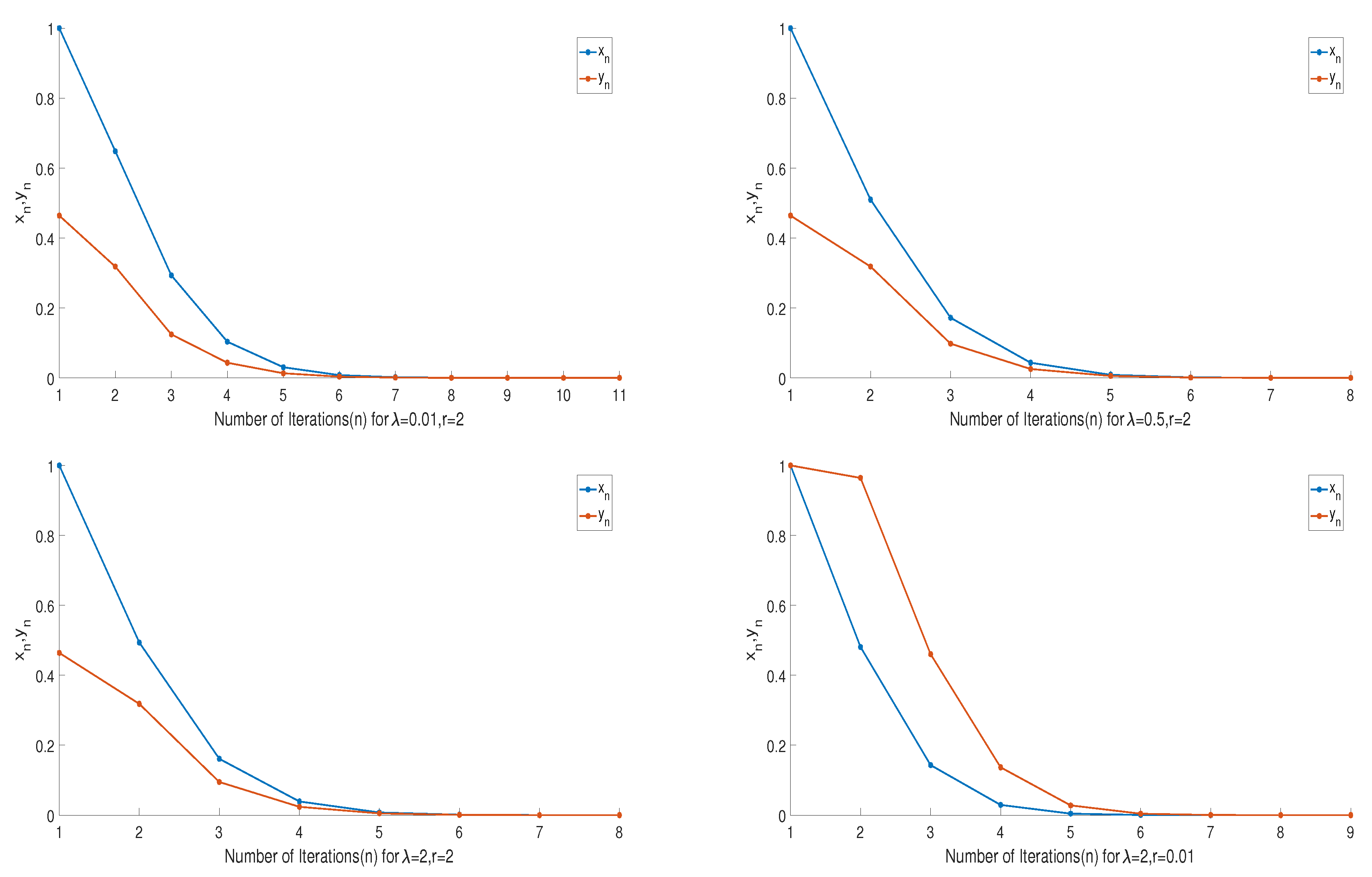
5.1. Numerical Behavior of Algorithm 1

Example 1.

Let $H_1=H_2=\mathbb{R}$ and define the operators $A,B_1$, and $B_2$ on real line $\mathbb{R}$ by $Ax=3x,B_{1}x=2x,B_{2}x=4x$ for all $x\in \mathbb{R}$, the bifunction ϕ by $\varphi (x,y)=-3x^2+xy+2y^2$ and set the parameters on Algorithm 1 by ${\rho }_n=3-\frac{1}{n+1}$, ${\alpha }_n=\frac{1}{n+1}$, ${\beta }_n=\frac{1}{{(n+1)}^2}$ for each $n\ge 1$. It is clear that

$${\mathsf{\Sigma }}_{n=1}^{\infty }|{\alpha }_n-{\alpha }_{n-1}|<\infty ,{\mathsf{\Sigma }}_{n=1}^{\infty }|{\beta }_n-{\beta }_{n-1}|<\infty ,\mathrm{EP}\left(\varphi \right)\bigcap \mathsf{\Omega }=\left\{0\right\}.$$

From the definition of ϕ, we have

$$\begin{array}{ccc}\hfill 0& \le & \varphi (z_n,y)+\frac{1}{r}⟨y-z_n,z_n-x_n⟩\hfill \\ & =& -3z_n^2+y{z}_n+2y^2+\frac{1}{r}(y-z_n)(z_n-x_n)\hfill \end{array}$$

(87)

and then

$$\begin{array}{ccc}\hfill 0& \le & r(-3z_n^2+y{z}_n+2y^2)+z_{n}y-z_n^2-x_{n}y+x_n{z}_n.\hfill \end{array}$$

(88)

For the quadratic function of y, if it has at most one solution in $\mathbb{R}$, then the discriminant of this function $\mathsf{\Delta }={(z_n+5z_{n}r-x_n)}^2=0$, that is, $z_n=\frac{x_n}{1+5r}$. According to Algorithm 1, if $\parallel G\left(y_n\right){\parallel }^2+{\parallel H\left(y_n\right)\parallel }^2\ne 0$, then we compute the new iteration $\left\{x_{n+1}\right\}$ and the iterative progress is written as

$$\begin{array}{c}\hfill \left\{\begin{array}{c}{z}_n=\frac{x_n}{1+5r},\hfill \\ y_n={\beta }_n{x}_n+(1-{\beta }_n)z_n,\hfill \\ x_{n+1}={\alpha }_n{x}_n+(1-{\alpha }_n)J_{\lambda }^{B_1}(I-{\gamma }_n{A}^{\ast }(I-J_{\lambda }^{B_2}A))y_n,\hfill \end{array}\right.\end{array}$$

In this way, the step size ${\gamma }_n$ is self-adaptive and not given beforehand.

First, we test three cases of $\lambda =0.01,0.5,2$ and $r=0.01,0.5,2$ for initial point $x_0=1$, and then test three initial points $x_0$ randomly generated by Matlab for λ and r. The values of $\left\{y_n\right\}$ and $\left\{x_n\right\}$ are reported in Figure 1 and Figure 2 and Table 1. In these figures, x-axes represent for the number of iterations while y-axes represent the value of $x_n$ and $y_n$, the stopping criterion of Figure 1 is $\parallel x_{n+1}-y_n\parallel ={10}^{-6}$. These figures imply that the behavior of $x_n$ for Algorithm 1 that converges to the same solution, i.e., $0\in \mathrm{EP}\left(\varphi \right)\bigcap \mathsf{\Omega }$ as a solution of this example.

Figure 1. Values of $x_n$ and $y_n$ for different $\lambda$ and r.

Figure 2. Values of $\parallel x_{n+1}-y_n\parallel$ and $x_n$.

Table 1. The convergence of Algorithm 1.

	${\mathit{x}}_0=-40$			${\mathit{x}}_0=50$
$\mathit{n}$	${\mathit{z}}_{\mathit{n}}$	${\mathit{y}}_{\mathit{n}}$	${\mathit{x}}_{\mathit{n}}$	${\mathit{z}}_{\mathit{n}}$	${\mathit{y}}_{\mathit{n}}$	${\mathit{x}}_{\mathit{n}}$
0	$-11.4286$	$-18.5714$	$-40$	14.2857	23.2143	50
1	$-5.6086$	$-7.1666$	$-19.6302$	7.0108	8.9582	24.5378
2	$-1.7934$	$-2.0736$	$-6.2767$	2.2417	2.5920	7.8459
3	$-0.4200$	$-0.620$	$-1.4700$	0.5250	0.5775	1.8374
4	$-0.0821$	$-0.0768$	$-0.2686$	0.0959	0.1026	0.3358
5	$-0.0114$	$-0.0120$	$-0.0399$	0.0142	0.0150	0.0498
6	$-0.0015$	$-0.0014$	$-0.0049$	0.0018	0.0018	0.0062
7	$-1.4847\times {10}^{-4}$	$-1.5305\times {10}^{-4}$	$-5.1964\times {10}^{-4}$	$1.8559\times {10}^{-4}$	$1.9131\times {10}^{-4}$	$6.4955\times {10}^{-4}$
8	$-1.3498\times {10}^{-5}$	$-1.3836\times {10}^{-5}$	$-4.7245\times {10}^{-5}$	$1.6873\times {10}^{-5}$	$1.7295\times {10}^{-5}$	$5.9056\times {10}^{-5}$
9	$-1.0716\times {10}^{-6}$	$-1.0938\times {10}^{-6}$	$-3.7507\times {10}^{-6}$	$1.3396\times {10}^{-6}$	$1.3672\times {10}^{-6}$	$4.6884\times {10}^{-6}$

We can summarize the following observations from these Figure 1 and Figure 2 and Table 1:

(1)

The results presented in Figure 1 and Figure 2 and Table 1 imply that Algorithm 1 converges to the same solution;

(2)

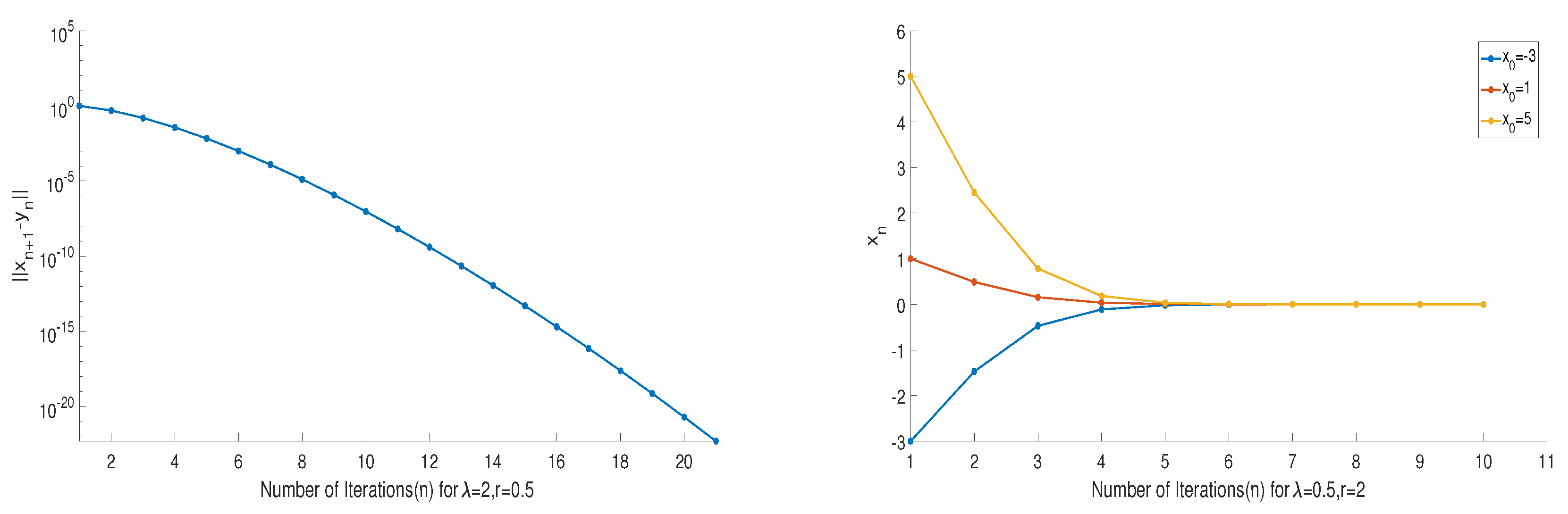
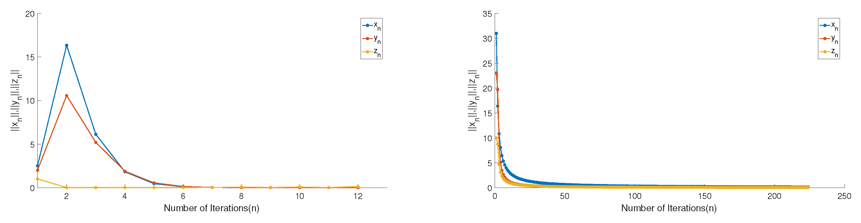
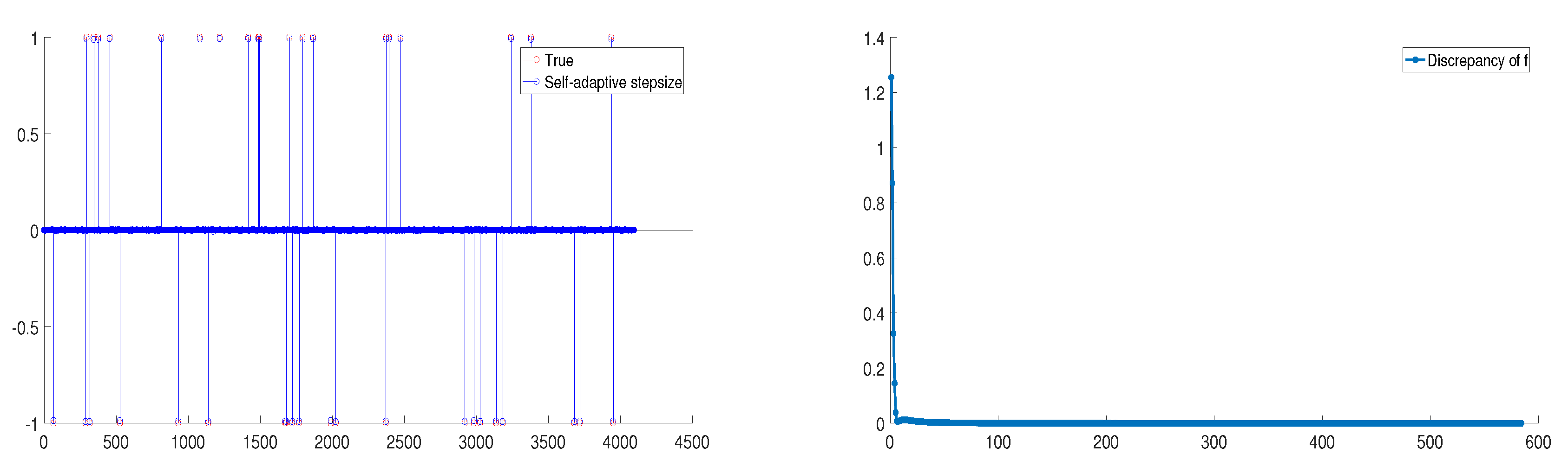
The convergence rate of Algorithm 1 is fast, efficient, stable and simple to implement. The number of iterations remains almost consistent irrespective of the initial point $x_0$ and parameters $\lambda ,r$.

(3)

The error of $\parallel x_{n+1}-y_n\parallel$ can be obtain approximately equal to ${10}^{-15}$ even smaller in 20 iterations.

5.2. Numerical Behaviours of Algorithms 2 and 3

Example 2.

Let $H_1=H_2={\mathbb{R}}^3$ and define the operators $A,B_1$, and $B_2$ as the following:

$$A=\left(\begin{array}{ccc}6& 3& 1\\ 8& 7& 5\\ 3& 6& 2\end{array}\right),B_1=\left(\begin{array}{ccc}6& 0& 0\\ 0& 4& 0\\ 0& 0& 3\end{array}\right),B_2=\left(\begin{array}{ccc}7& 0& 0\\ 0& 5& 0\\ 0& 0& 2\end{array}\right),$$

the bifunction ϕ by $\varphi (x,y)=-3x^2+⟨x,y⟩+2y^2$. In this example, we set the parameters in Algorithm 2 and Algorithm 3 by ${\alpha }_n=\frac{n}{n+1}$, ${\rho }_n=3-\frac{1}{n+1}$, ${\tau }_n=\frac{1}{{(n+1)}^2}$, and ${\beta }_n=\frac{1}{(n+1)}$ for each $n\ge 1$.

First, we take an initial point $x_0=(13,-12,25)$, then the test results are reported in Figure 3.

Figure 3. Values of $\parallel x_n\parallel ,\parallel y_n\parallel ,\parallel z_n\parallel$ for Algorithms 2 and 3.

Next, we present the test results for initial point $x_0=(1,-1,-2)$ in Table 2.

Table 2. The convergence of Algorithm 3.

n	${\mathit{x}}_{\mathit{n}}$	${\mathit{y}}_{\mathit{n}}$	$\parallel {\mathit{x}}_{\mathit{n}}\parallel$	$\parallel {\mathit{y}}_{\mathit{n}}\parallel$
0	$(1,-1,2)$	$(0.6429,-0.6429,1.2857)$	2.4490	1.5747
1	$(0.2561,-0.3074,0.5742)$	$(0.1341,-0.1610,0.3008)$	0.6998	0.3666
2	$(0.0582,-0.0866,0.1509)$	$(0.0270,-0.0402,0.0701)$	0.1835	0.0852
3	$(0.0111,-0.0211,0.0345)$	$(0.0048,-0.0090,0.0148)$	0.0419	0.0180
4	$(0.0018,-0.0045,0.0069)$	$(0.0007,-0.0018,0.0028)$	0.0084	0.0034
5	$(0.0002,-0.0008,0.0012)$	$(9.17\times {10}^{-4},-3.274\times {10}^{-4},4.805\times {10}^{-4})$	0.0015	$5.8868\times {10}^{-4}$
6	$(1.93\times {10}^{-5},-1.443\times {10}^{-4},1.936\times {10}^{-4})$	$(7.25\times {10}^{-6},-5.413\times {10}^{-5},7.261\times {10}^{-5})$	$2.4229\times {10}^{-4}$	$9.0860\times {10}^{-5}$
7	$(4.21\times {10}^{-6},-1.672\times {10}^{-5},3.119\times {10}^{-5})$	$(1.54\times {10}^{-6},-6.10\times {10}^{-6},1.139\times {10}^{-5})$	$3.5640\times {10}^{-5}$	$1.3011\times {10}^{-5}$
8	$(2.98\times {10}^{-7},-2.483\times {10}^{-6},4.284\times {10}^{-6})$	$(1.07\times {10}^{-7},-8.87\times {10}^{-7},1.530\times {10}^{-6})$	$4.9606\times {10}^{-6}$	$1.7716\times {10}^{-6}$
9	$(-2.33\times {10}^{-8},-3.472\times {10}^{-7},5.032\times {10}^{-7})$	$(-8.2\times {10}^{-9},-1.217\times {10}^{-7},1.764\times {10}^{-7})$	$6.1179\times {10}^{-7}$	$2.1458\times {10}^{-7}$

From Table 2 and Figure 3, one can see the convergence rate of Algorithm 3 is faster than Algorithm 2 and $(0,0,0)\in \mathrm{EP}\left(\varphi \right)\bigcap \mathsf{\Omega }$ is the minimum-norm solution of the experiment.

5.3. Comparisons with Other Algorithms

In this part, we present several experiments in comparison our Algorithms 1 and 3 with the other algorithms. Two methods used to compare are the algorithm in Byrne et al. [36] and the algorithm in Sitthithakerngkiet et al. [46]. The step size $\gamma \equiv 0.001$ for the algorithm in Byrne et al. [36] and the algorithm in Sitthithakerngkiet et al. [46] which depends on the norm of operator A. In addition, let the mapping $S_n:{\mathbb{R}}^3\to {\mathbb{R}}^3$ be an infinite family of nonexpansive mappings $S_n\left(x\right)=\left\{\frac{x}{2^n}\right\}$ and a nonnegative real sequence ${\zeta }_n=1$. Then the W-mapping $W_n$ is generated by $S_n$ and ${\zeta }_n$ and $W_n=\frac{1}{2^{\frac{n(n+1)}{2}}}$, the bounded linear operator $D=I$ in Sitthithakerngkiet et al. [46]. We choose the stopping criterion for our algorithm is $\parallel x_{n+1}-y_n\parallel \le \mathrm{DOL}$, for Byrne et al. [36] is $\parallel x_{n+1}-x_n\parallel \le \mathrm{DOL}$ and for Sitthithakerngkiet et al. [46] is $\parallel x_{n+1}-y_n\parallel \le \mathrm{DOL}$. For the three algorithms, the operators $A,B_1,B_2$ are defined as Example 2, the parameters ${\alpha }_n=\frac{{10}^{-3}}{n}$ and ${\beta }_n=0.5-\frac{1}{10n+2}$, $u=(0,0,1)$ in Sitthithakerngkiet et al. [46], ${\rho }_n=3-\frac{1}{n+1}$, ${\alpha }_n=\frac{1}{n+1}$ and ${\beta }_n=\frac{1}{10n+2}$ in our Algorithm 1, ${\rho }_n=3-\frac{1}{n+1}$, ${\alpha }_n=\frac{n}{n+1}$ and ${\beta }_n=\frac{1}{10n+2}$ in our Algorithm 3. We take $\lambda =1$, $x_0=(13,-12,25)$ for all these algorithms and compare the iterations and computer times. The experiment results are reported in Table 3.

Table 3. Comparison Algorithms 1 and 3 with other algorithms.

DOL	Method	Step Size	Iteration (n)	CPU Time (s)	$\frac{\parallel \mathit{z}-{\mathit{x}}_{\mathit{n}}\parallel }{\parallel {\mathit{x}}_0-{\mathit{x}}_{\mathit{n}+1}\parallel }$
${10}^{-4}$	Algorithm 1	${\gamma }_n=\frac{{\rho }_n(f\left(y_n\right)+g\left(y_n\right))}{\parallel F\left(y_n\right){\parallel }^2+{\parallel G\left(y_n\right)\parallel }^2}$	9	0.10002	$1.1393\times {10}^{-4}$
	Algorithm 3	${\gamma }_n=\frac{{\rho }_n(f\left(y_n\right)+g\left(y_n\right))}{\parallel F\left(y_n\right){\parallel }^2+{\parallel G\left(y_n\right)\parallel }^2}$	8	0.0898	$1.2675\times {10}^{-4}$
	Sitthithakerngkiet et al. [46]	$\gamma =0.001$	23	0.086643	$5.4438\times {10}^{-6}$
	Byrne et al. [36]	$\gamma =0.001$	10	0.087847	$1.8355\times {10}^{-6}$
${10}^{-5}$	Algorithm 1	${\gamma }_n=\frac{{\rho }_n(f\left(y_n\right)+g\left(y_n\right))}{\parallel F\left(y_n\right){\parallel }^2+{\parallel G\left(y_n\right)\parallel }^2}$	11	0.11003	$2.9283\times {10}^{-6}$
	Algorithm 3	${\gamma }_n=\frac{{\rho }_n(f\left(y_n\right)+g\left(y_n\right))}{\parallel F\left(y_n\right){\parallel }^2+{\parallel G\left(y_n\right)\parallel }^2}$	10	0.109419	$3.2668\times {10}^{-6}$
	Sitthithakerngkietet et al. [46]	$\gamma =0.001$	218	0.104271	$5.2318\times {10}^{-7}$
	Byrne et al. [36]	$\gamma =0.001$	12	0.092779	$1.0173\times {10}^{-7}$
${10}^{-6}$	Algorithm 1	${\gamma }_n=\frac{{\rho }_n(f\left(y_n\right)+g\left(y_n\right))}{\parallel F\left(y_n\right){\parallel }^2+{\parallel G\left(y_n\right)\parallel }^2}$	12	0.116322	$4.4459\times {10}^{-7}$
	Algorithm 3	${\gamma }_n=\frac{{\rho }_n(f\left(y_n\right)+g\left(y_n\right))}{\parallel F\left(y_n\right){\parallel }^2+{\parallel G\left(y_n\right)\parallel }^2}$	11	0.119499	$4.4445\times {10}^{-7}$
	Sitthithakerngkietet et al. [46]	$\gamma =0.001$	2171	0.768808	$5.2142\times {10}^{-8}$
	Byrne et al. [36]	$\gamma =0.001$	13	0.084488	$2.3954\times {10}^{-8}$

From all the above figures and tables, one can see the behavior of the sequences $\left\{x_n\right\}$ and $\left\{y_n\right\}$, which concludes that $\left\{x_n\right\}$ and $\left\{y_n\right\}$ converge to a solution and our algorithms are fast, efficient, and stable and simple to implement (it takes average of 10 iterations to converge). Especially, one can see that our Algorithms 1 and 3 seem to have a competitive advantage. However, as mentioned in the previous sections, the main advantage of these our algorithms is that the step size is self-adaptive without the prior knowledge of operator norms.

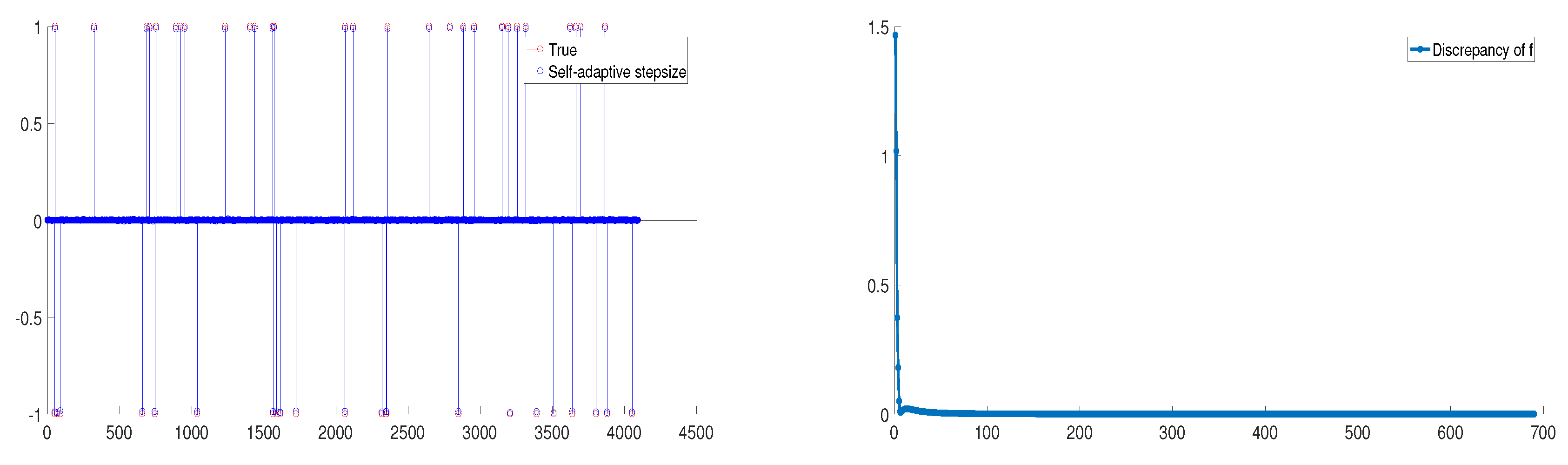
5.4. Compressed Sensing

In the last example, we choose a problem from the field of compressed sensing according to the review comments, that is the recovery of a sparse and noisy signal from a limited number of sampling. Let $x_0\in {\mathbb{R}}^n$ be K-sparse signal, $K<<n$. The sampling matrix $A\in R^{m\times n},m<n$ is stimulated by standard Gaussian distribution and vector $b=Ax+ϵ$, where $ϵ$ is additive noise. When $ϵ=0$, it means that there is no noise to the observed data. Our task is to recover the signal $x_0$ from the data b. For further details, one can consult with Nguyen and Shin [34].

For solving the problem, we recall the LASSO (Least Absolute Shrink Select Operator) problem Tibshirani [60] as follows:

$$\begin{array}{c}\underset{x\in R^n}{min}\frac{1}{2}{\parallel Ax-b\parallel }_2^2\\ {\mathrm{s}.\mathrm{t}.\parallel x\parallel }_1\le t,\end{array}$$

where $t>0$ is a given constant. So, in the relation with the problem SVIPs (5) and (6), we consider $B_1^{-1}\left(0\right)={\left\{x\right|\parallel x\parallel }_1\le t\}$, $B_2^{-1}\left(0\right)=\left\{b\right\}$ and define

$$\begin{array}{c}\hfill B_1\left(x\right)=\left\{\begin{array}{cc}\{u|{sup}_{{\parallel y\parallel }_1\le t}⟨y-x,u⟩\le 0\},\hfill & x\in C,\hfill \\ \varnothing ,\hfill & \mathrm{otherwise}.\hfill \end{array}\right.\end{array}$$

and define

$$\begin{array}{c}\hfill B_2\left(y\right)=\left\{\begin{array}{cc}{H}_2,\hfill & y=b,\hfill \\ \varnothing ,\hfill & \mathrm{otherwise}.\hfill \end{array}\right.\end{array}$$

In this example, we take $h\left(x\right)=\frac{1}{2}{\parallel Ax-b\parallel }^2$, $\varphi (x,y)=h\left(y\right)-h\left(x\right)$, then the problem EP (1) is equivalent to the following problem:

$$\underset{x\in R^n}{min}\frac{1}{2}{\parallel Ax-b\parallel }_2^2.$$

For the experiment setting, we choose the following parameters in our Algorithm 3: ${\alpha }_i=\frac{i-1}{i+1}$, ${\gamma }_i=\frac{1}{i+1}$, ${\beta }_i=\frac{2i-1}{2i+1}$, ${\rho }_i=3-\frac{1}{i+1}$, $A\in {\mathbb{R}}^{m\times n}$ is generated randomly with $m=2^{10}$, $n=2^{12}$, $x_0\in {\mathbb{R}}^n$ is K-spikes with amplitude $\pm 1$ distributed in whole domain randomly. In addition, for simplicity, we take $t=K$ and the stopping criterion $\parallel x_{i+1}-x_i\parallel \le \mathrm{DOL}$ with $\mathrm{DOL}={10}^{-6}$. All the numerical results are presented in Figure 4 and Figure 5.

Figure 4. Numerical result for $K=50$.

Figure 5. Numerical result for $K=40$.

6. Conclusions

A series of some problems in finance, physics, network analysis, signal processing, image reconstruction, economics, and optimizations are reduced to find a common solution of the split inverse and equilibrium problems, which implies numerous possible applications to mathematical models whose constraints can be presented as the problem EP (1) and the split inverse problem.

This motivated the study of a common solution set of split variational inclusion problems and equilibrium problems.

The main result of this paper is to introduce a new self-adaptive step size algorithm without prior knowledge of the operator norms in Hilbert spaces to solve the split variational inclusion and equilibrium problems. The convergence theorems are obtained under suitable assumptions and the numerical examples and comparisons are presented to illustrate the efficiency and reliability of the algorithms. In one sense, the algorithms and theorems in this paper complement, extend, and unify some related results in the split variational inclusion and equilibrium problems.

References

- Blum, E.; Oettli, W. From optimization and variational inequalities to equilibrium problems. Math. Stud. 1994, 63, 123–145. [Google Scholar]
- Flam, D.S.; Antipin, A.S. Equilibrium programming using proximal-like algorithms. Math. Program. 1997, 78, 29–41. [Google Scholar] [CrossRef]
- Moudafi, A. Second-order differential proximal methods for equilibrium problems. J. Inequal. Pure Appl. Math. 2003, 4, 18. [Google Scholar]
- Bnouhachem, A.; Suliman, A.H.; Ansari, Q.H. An iterative method for common solution of equilibrium problems and hierarchical fixed point problems. Fixed Point Theory Appl. 2014, 2014, 194. [Google Scholar] [CrossRef]
- Konnov, I.V.; Ali, M.S.S. Descent methods for monotone equilibrium problems inBanach spaces. J. Comput. Appl. Math. 2006, 188, 165–179. [Google Scholar] [CrossRef]
- Konnov, I.V.; Pinyagina, O.V. D-gap functions and descent methods for a class of monotone equilibrium problems. Lobachevskii J. Math. 2003, 13, 57–65. [Google Scholar]
- Charitha, C. A Note on D-gap functions for equilibrium problems. Optimization 2013, 62, 211–226. [Google Scholar] [CrossRef]
- Lorenzo, D.D.; Passacantando, M.; Sciandrone, M. A convergent inexact solution method for equilibrium problems. Optim. Methods Softw. 2014, 29, 979–991. [Google Scholar] [CrossRef]
- Ceng, L.C.; Ansari, Q.H.; Yao, J.C. Some iterative methods for finding fixed point and for solving constrained convex minimization problems. Nonlinear Anal. 2011, 74, 5286–5302. [Google Scholar] [CrossRef]
- Yao, Y.; Cho, Y.J.; Liou, Y.C. Iterative algorithm for hierarchical fixed points problems and variational inequalities. Math. Comput. Model. 2010, 52, 1697–1705. [Google Scholar] [CrossRef]
- Yao, Y.; Cho, Y.J.; Liou, Y.C. Algorithms of common solutions for variational inclusions, mixed equilibrium problems and fixed point problems. Eur. J. Oper. Res. 2011, 212, 242–250. [Google Scholar] [CrossRef]
- Yao, Y.H.; Liou, Y.C.; Yao, J.C. New relaxed hybrid-extragradient method for fixed point problems, a general system of variational inequality problems and generalized mixed equilibrium problems. Optimization 2011, 60, 395–412. [Google Scholar] [CrossRef]
- Qin, X.; Chang, S.S.; Cho, Y.J. Iterative methods for generalized equilibrium problems and fixed point problems with applications. Nonlinear Anal. Real World Appl. 2010, 11, 2963–2972. [Google Scholar] [CrossRef]
- Qin, X.; Cho, Y.J.; Kang, S.M. Viscosity approximation methods for generalized equilibrium problems and fixed point problems with applications. Nonlinear Anal. 2010, 72, 99–112. [Google Scholar] [CrossRef]
- Hung, P.G.; Muu, L.D. For an inexact proximal point algorithm to equilibrium problem. Vietnam J. Math. 2012, 40, 255–274. [Google Scholar]
- Quoc, T.D.; Muu, L.D.; Nguyen, V.H. Extragradient algorithms extended to equilibrium problems. Optimization 2008, 57, 749–776. [Google Scholar] [CrossRef]
- Santos, P.; Scheimberg, S. An inexact subgradient algorithm for equilibrium problems. Comput. Appl. Math. 2011, 30, 91–107. [Google Scholar]
- Thuy, L.Q.; Anh, P.K.; Muu, L.D.; Hai, T.N. Novel hybrid methods for pseudomonotone equilibrium problems and common fixed point problems. Numer. Funct. Anal. Optim. 2017, 38, 443–465. [Google Scholar] [CrossRef]
- Rockafellar, R.T. Monotone operators and proximal point algorithm. SAIM J. Control Optim. 1976, 14, 877–898. [Google Scholar] [CrossRef]
- Moudafi, A. From alternating minimization algorithms and systems of variational inequalities to equilibrium problems. Commun. Appl. Nonlinear Anal. 2019, 16, 31–35. [Google Scholar]
- Moudafi, A. Proximal point algorithm extended to equilibrium problem. J. Nat. Geometry 1999, 15, 91–100. [Google Scholar]
- Muu, L.D.; Otelli, W. Convergence of an adaptive penalty scheme for finding constrained equilibria. Nonlinear Anal. 1992, 18, 1159–1166. [Google Scholar] [CrossRef]
- Dong, Q.L.; Tang, Y.C.; Cho, Y.J.; Rassias, T.M. “Optimal” choice of the step length of the projection and contraction methods for solving the split feasibility problem. J. Glob. Optim. 2018, 71, 341–360. [Google Scholar] [CrossRef]
- Censor, Y.; Elfving, T. A multiprojection algorithm using Bregman projections in a product space. Numer. Algorithms 1994, 8, 221–239. [Google Scholar] [CrossRef]
- Ansari, Q.H.; Rehan, A. Split feasibility and fixed point problems. In Nonlinear Analysis, Approximation Theory, Optimization and Applications; Springer: Berlin/Heidelberg, Germany, 2014; pp. 281–322. [Google Scholar]
- Xu, H.K. Iterative algorithms for nonliear operators. J. Lond. Math. Soc. 2002, 66, 240–256. [Google Scholar] [CrossRef]
- Qin, X.; Shang, M.; Su, Y. A general iterative method for equilibrium problems and fixed point problems in Hilbert spaces. Nonlinear Anal. 2008, 69, 3897–3909. [Google Scholar] [CrossRef]
- Ceng, L.C.; Ansari, Q.H.; Yao, J.C. An extragradient method for solving split feasibility and fixed point problems. Comput. Math. Appl. 2012, 64, 633–642. [Google Scholar] [CrossRef]
- Censor, Y.; Bortfeld, T.; Martin, B.; Trofimov, A. A unified approach for inversion problems in intensity modulated radiation therapy. Phys. Med. Biol. 2003, 51, 2353–2365. [Google Scholar] [CrossRef]
- Kazmi, K.R.; Rizvi, S.H. An iterative method for split variational inclusion problem and fixed point problem for a nonexpansive mapping. Optim. Lett. 2014, 8, 1113–1124. [Google Scholar] [CrossRef]
- Censor, Y.; Gibali, A.; Reich, S. Algorithms for the split variational inequality problem. Numer. Algorithms 2012, 59, 301–323. [Google Scholar] [CrossRef]
- Moudafi, A. The split common fixed point problem for demicontractive mappings. Inverse Probl. 2010, 26, 587–600. [Google Scholar] [CrossRef]
- Moudafi, A. Split monotone variational inclusions. J. Optim. Theory Appl. 2011, 150, 275–283. [Google Scholar] [CrossRef]
- Nguyen, T.L.; NShin, Y. Deterministic sensing matrices in compressive sensing: A survey. Sci. World J. 2013, 2013, 1–6. [Google Scholar] [CrossRef]
- Dang, Y.; Gao, Y. The strong convergence of a KM-CQ-like algorithm for a split feasibility problem. Inverse Probl. 2011, 27, 015007. [Google Scholar] [CrossRef]
- Byrne, C.; Censor, Y.; Gibali, A.; Reich, S. Weak and strong convergence of algorithms for the split common null point problem. J. Nonlinear Convex Anal. 2012, 13, 759–775. [Google Scholar]
- Byrne, C. Iterative oblique projection onto convex sets and the split feasibility problem. Inverse Probl. 2002, 18, 441–453. [Google Scholar] [CrossRef]
- Byrne, C. A unified treatment of some iterative algorithms in signal processing and image reconstruction. Inverse Probl. 2004, 20, 103–120. [Google Scholar] [CrossRef]
- Yang, Q. The relaxed CQ algorithm for solving the split feasibility problem. Inverse Probl. 2004, 20, 1261–1266. [Google Scholar] [CrossRef]
- Gibali, A.; Mai, D.T.; Nguyen, T.V. A new relaxed CQ algorithm for solving split feasibility problems in Hilbert spaces and its applications. J. Ind. Manag. Optim. 2018, 2018, 1–25. [Google Scholar]
- López, G.; Martin-Marquez, V.; Xu, H.K. Solving the split feasibility problem without prior knowledge of matrix norms. Inverse Probl. 2012, 28, 085004. [Google Scholar] [CrossRef]
- Moudafi, A.; Thukur, B.S. Solving proximal split feasibility problem without prior knowledge of matrix norms. Optim. Lett. 2013, 8. [Google Scholar] [CrossRef]
- Gibali, A. A new split inverse problem and application to least intensity feasible solutions. Pure Appl. Funct. Anal. 2017, 2, 243–258. [Google Scholar]
- Plubtieng, S.; Sombut, K. Weak convergence theorems for a system of mixed equilibrium problems and nonspreading mappings in a Hilbert space. J. Inequal. Appl. 2010, 2010, 246237. [Google Scholar] [CrossRef]
- Sombut, K.; Plubtieng, S. Weak convergence theorem for finding fixed points and solution of split feasibility and systems of equilibrium problems. Abstr. Appl. Anal. 2013, 2013, 430409. [Google Scholar] [CrossRef]
- Sitthithakerngkiet, K.; Deepho, J.; Martinez-Moreno, J.; Kuman, P. Convergence analysis of a general iterative algorithm for finding a common solution of split variational inclusion and optimization problems. Numer. Algorithms 2018, 79, 801–824. [Google Scholar] [CrossRef]
- Eslamian, M.; Fakhri, A. Split equality monotone variational inclusions and fixed point problem of set-valued operator. Acta Univ. Sapientiaemath. 2017, 9, 94–121. [Google Scholar] [CrossRef]
- Censor, Y.; Segal, A. The split common fixed point problem for directed operators. J. Convex Anal. 2019, 16, 587–600. [Google Scholar]
- Plubtieng, S.; Sriprad, W. A viscosity approximation method for finding common solutions of variational inclusions, equilibrium problems, and fixed point problems in Hilbert spaces. Fixed Point Theory Appl. 2009, 2009, 567147. [Google Scholar] [CrossRef]
- Mainge, P.E. Strong convergence of projected subgradient methods for nonsmooth and nonstrictly convex minimization. Set-Valued Anal. 2008, 16, 899–912. [Google Scholar] [CrossRef]
- Bruck, R.E.; Reich, S. Nonexpansive projections and resolvents of accretive operators in Banach spaces. Houst. J. Math. 1977, 3, 459–470. [Google Scholar]
- Mainge, P.E. Approximation methods for common fixed points of nonexpansive mappings in Hilbert spaces. J. Math. Anal. Appl. 2007, 325, 469–479. [Google Scholar] [CrossRef]
- Osilike, M.O.; Aniagbosor, S.C.; Akuchu, G.B. Fixed point of asymptotically demicontractive mappings in arbitrary Banach spaces. PanAm. Math. J. 2002, 12, 77–88. [Google Scholar]
- Goebel, K.; Kirk, W.A. Topics in Metric Fixed Point Theory; Cambridge University Press: Cambridge, UK, 1990. [Google Scholar]
- Aubin, J.P. Optima and Equilibria: An Introduction to Nonlinear Analysis; Springer: Berlin/Heidelberg, Germany, 1993. [Google Scholar]
- Ishikawa, S. Fixed points and iteration of a nonexpansive mapping in Banach space. Proc. Am. Math. Soc. 1976, 59, 65–71. [Google Scholar] [CrossRef]
- Browder, F.E.; Petryshyn, W.V. The solution by iteration of nonlinear functional equations in Banach spaces. Bull. Am. Math. Soc. 1966, 72, 571–575. [Google Scholar] [CrossRef]
- Baillon, J.B.; Bruck, R.E.; Reich, S. On the asymptotic behavior of nonexpansive mappings and semigroups in Banach spaces. Houst. J. Math. 1978, 4, 1–9. [Google Scholar]
- Rockafellar, R.T. On the maximal monotonicity of subdifferential mappings. Pac. J. Math. 1970, 33, 209–216. [Google Scholar] [CrossRef]
- Tibshirani, R. Regression shrinkage and selection via the Lasso. J. R. Stat. Soc. 1996, 58, 267–288. [Google Scholar] [CrossRef]
© 2019 by the authors. Licensee MDPI, Basel, Switzerland. This article is an open access article distributed under the terms and conditions of the Creative Commons Attribution (CC BY) license (http://creativecommons.org/licenses/by/4.0/).