Discussion of “Accurate and Efficient Explicit Approximations of the Colebrook Flow Friction Equation Based on the Wright ω-Function” by DejanBrkić; and Pavel Praks, Mathematics 2019, 7, 34; doi:10.3390/math7010034

Abstract

The Colebrook-White equation is often used for calculation of the friction factor in turbulent regimes; it has succeeded in attracting a great deal of attention from researchers. The Colebrook–White equation is a complex equation where the computation of the friction factor is not direct, and there is a need for trial-error methods or graphical solutions; on the other hand, several researchers have attempted to alter the Colebrook-White equation by explicit formulas with the hope of achieving zero-percent (0%) maximum deviation, among them Dejan Brkić and Pavel Praks. The goal of this paper is to discuss the results proposed by the authors in their paper:” Accurate and Efficient Explicit Approximations of the Colebrook Flow Friction Equation Based on the Wright ω-Function” and to propose more accurate formulas.

1. Introduction

In the discussed paper, Dejan Brkić and Pavel Praks [1] presented a new formula, where they claim that the error recorded is about 0.0096% for the entire range of the relative roughness, and the Reynolds number is given by the following ranges: $0\le \left(\epsilon /D\right)\le 0.05$ and $4000\le R_e\le {10}^8$.

The discussion in this paper adds a number of comments about the results of the authors and proposes exact formulas.

2. Comments about the Results

The Colebrook-White equation is an empirical formula; it is given by Equation (1) [2]:

$$f={\left[-2\log \left(\frac{\epsilon /D}{3.71}+\frac{2.51}{R_e\sqrt{f}}\right)\right]}^{-2}$$

(1)

where

• ε is the average roughness height (or the equivalent Nikuradse sand-grain roughness),
• D is the inner pipe diameter,
• f is the friction factor,
• and Re is the Reynolds number.

Equation (1) implicitly needs iterative methods or a graphical solution such as the Moody diagram. The iterative methods require a great deal of time, and the graphical solutions are not accurate and are limited. To alter the implicit Colebrook-White equation, several authors have proposed an explicit solution to avoid such difficulties and weaknesses in the above methods [3].

The authors have proposed a new explicit solution using the Wright ω-function which is more numerically stable compared to the lumber function [4,5].

Firstly, the authors have proposed Equation (2) as follows:

$$\frac{1}{\sqrt{f}}\approx 0.8686\left[B-C+\frac{C}{B+A}\right]$$

(2)

$$A\approx \frac{R{\epsilon }^{*}}{8.0878}$$

$$B\approx ln\left(R\right)-0.779397488$$

$$C=ln\left(B+A\right)$$

For more accuracy, Equations (3) and (4) are proposed:

$$\frac{1}{\sqrt{f}}\approx 0.8686\left[B-C+\frac{1.038.C}{0.332+B+A}\right]$$

(3)

$$\frac{1}{\sqrt{f}}\approx 0.8686\left[B-C+\frac{1.0119.C}{B+A}+\frac{C-2.3849}{{\left(B+A\right)}^2}\right]$$

(4)

where parameters A, B and C are the same as in Equation (2).

The authors claimed that the maximum deviations recorded using Equation (2) is about only 0.13% and 0.009% for Equation (4).

The authors recommend the use of A7 for the approximation of B to get a negligible relative error of 0.007% compared with calculating B using Equation (2).

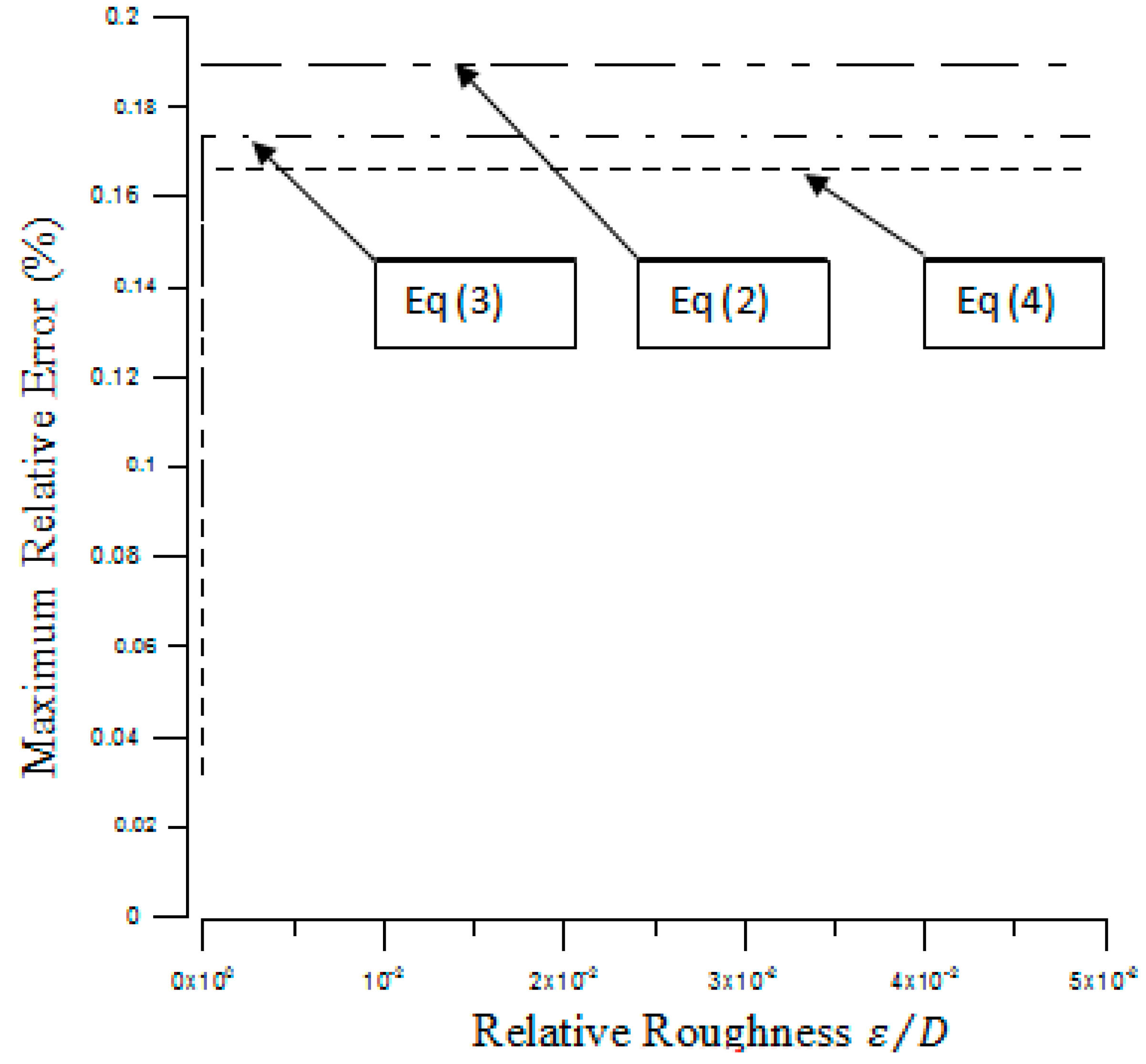
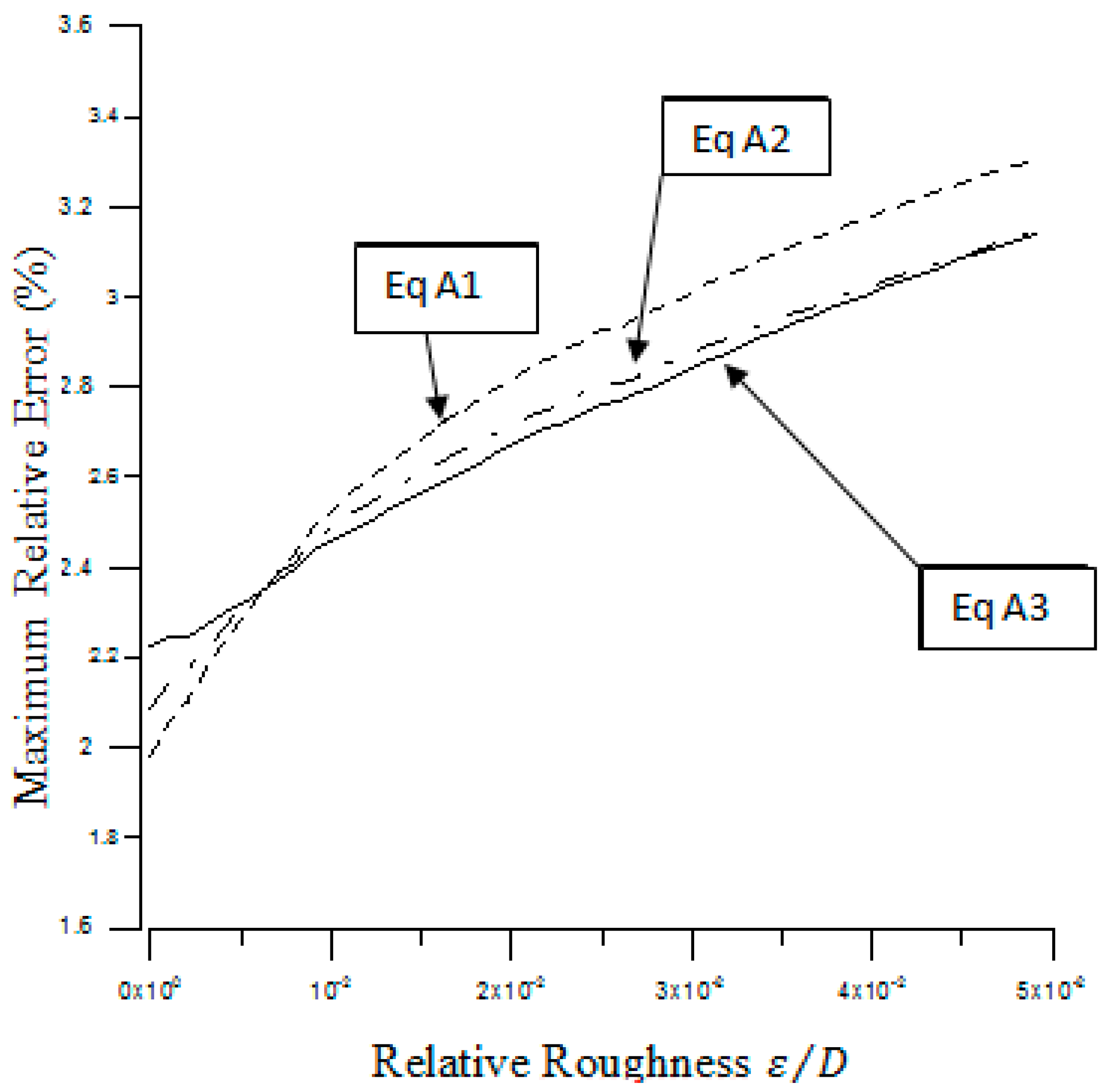
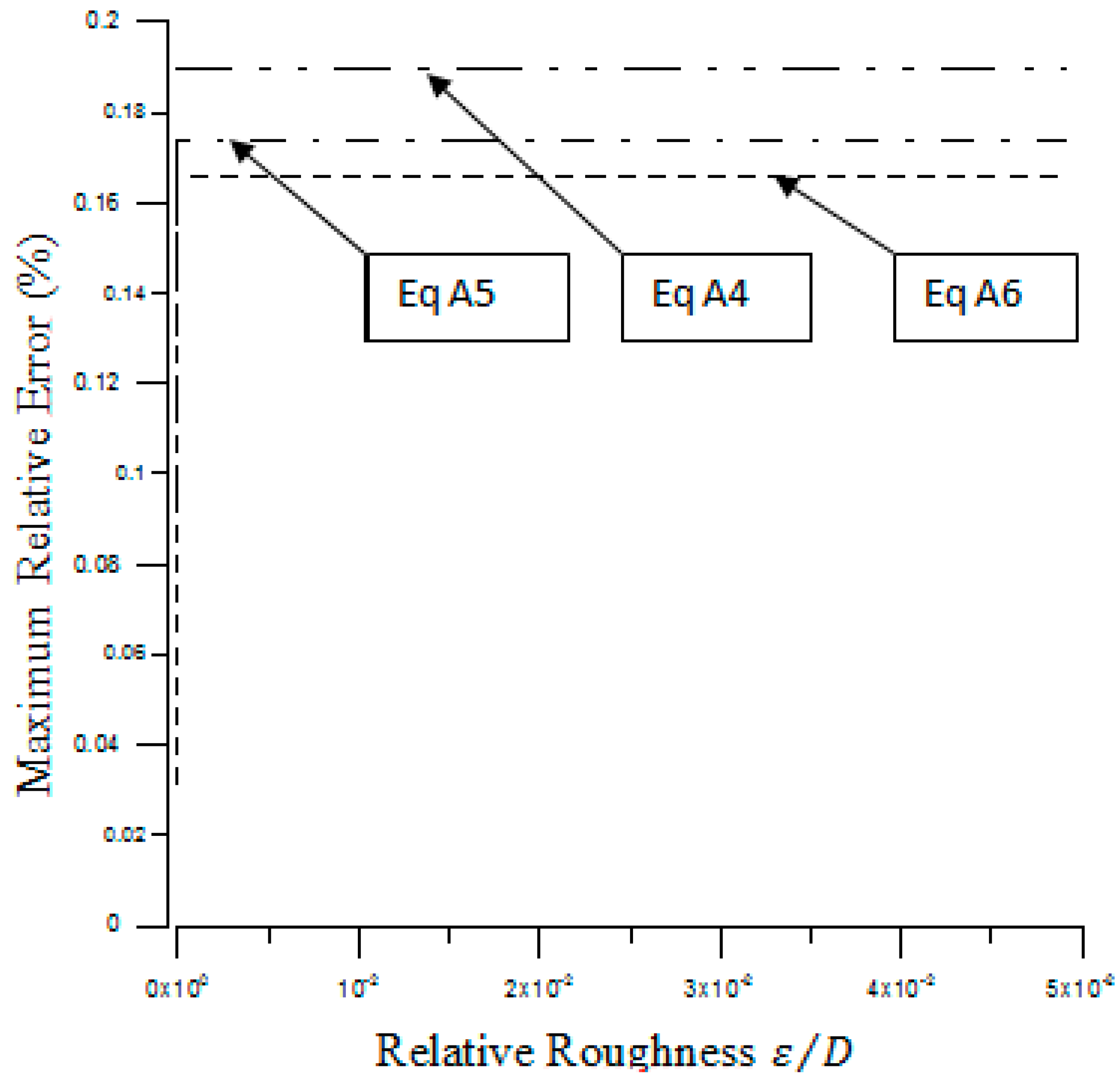
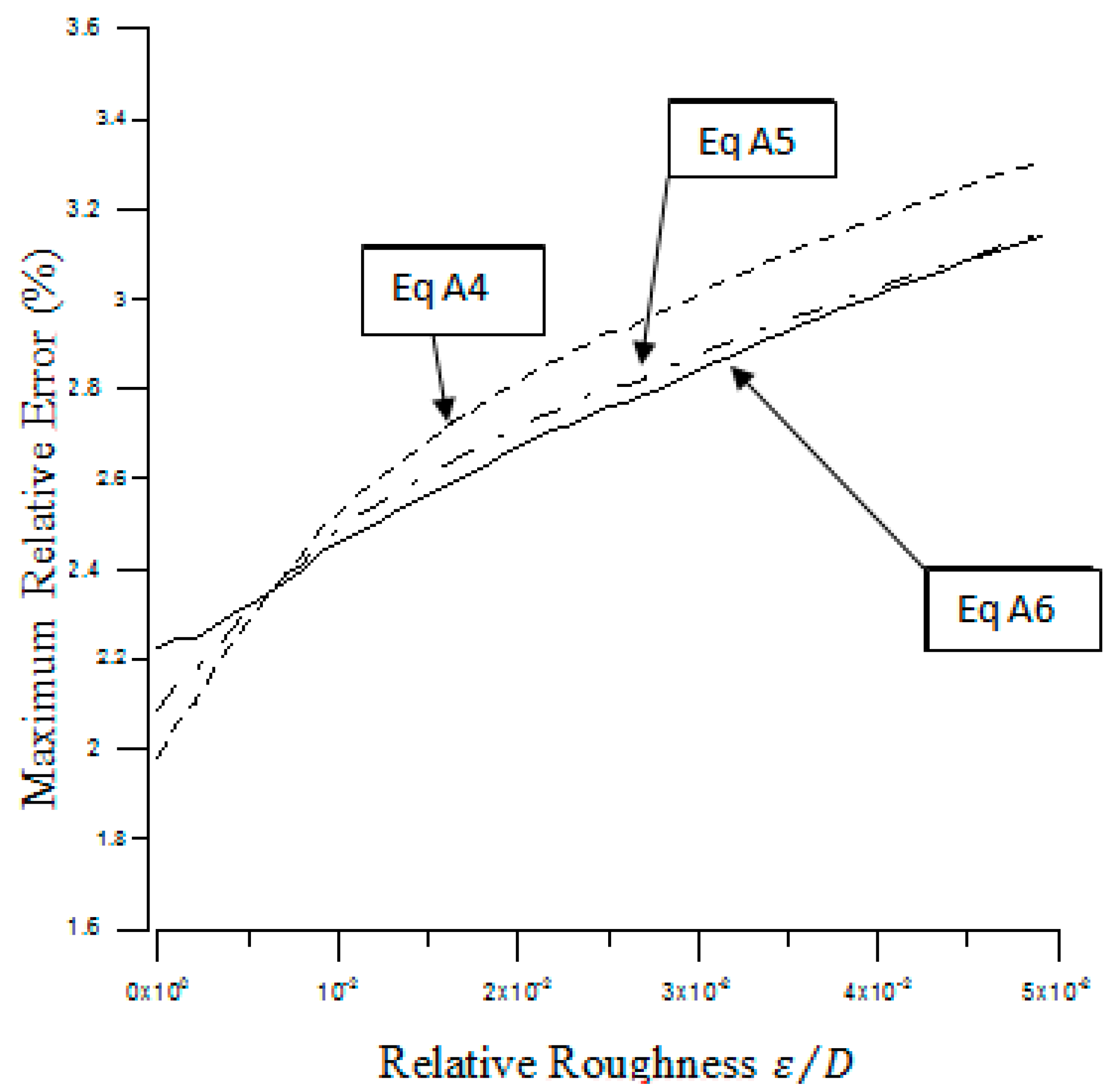
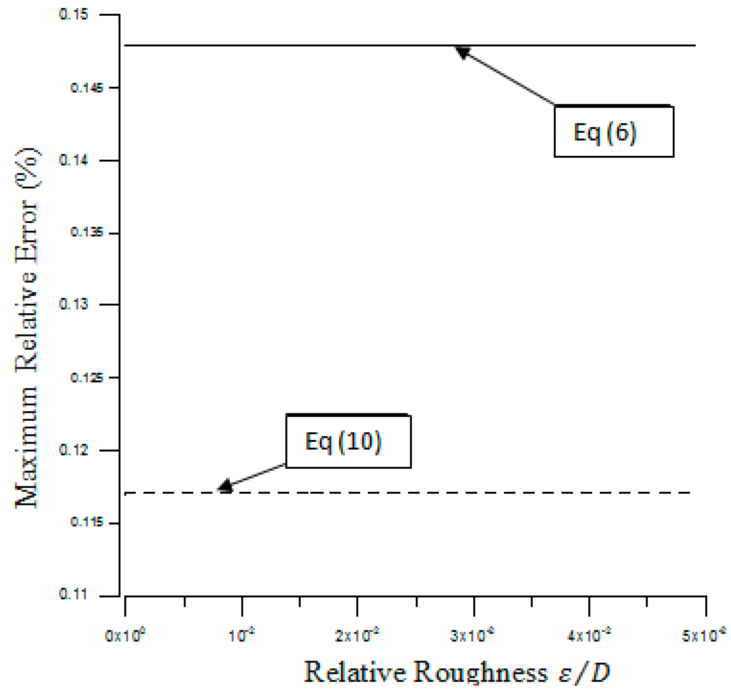
3. Accuracy Assessment

Three criteria were proposed by Zeghadnia et al. (2019) [3] to assess the accuracy of the explicit solutions for the turbulent flow friction factor, where many steps must be followed:

• The random value of relative roughness is selected from the range

  $$0\le \frac{\epsilon }{D}\le 0.05;$$
• The Reynolds number is within the entire range proposed by the authors,

  $$4000\le R_e\le {10}^8;$$
• Each value of the relative roughness of the friction factor is calculated using the Colebrook-White formula iteratively for all values of the Reynolds number;
• The friction factor for each approximation cited above will be calculated using the appropriate proposed equation;
• The relative error $\left(\Delta f/f\right)$ in (%) between the friction factors $f_{\mathrm{proposed}}$ and $f_{\mathrm{CW}}$, which respectively mean the proposed formula and Colebrook–White equation, is easily computed using the following formula:

  $$\frac{\Delta f}{f}=100\%\left(\frac{f_{\mathrm{proposed}}-f_{\mathrm{CW}}}{f_{\mathrm{CW}}}\right);$$

  (5)
• Equations (2)–(4) and (A4)–(A6) will be tested using the formulas of B, which are:

  ✔

  Formula of B in Equations 2(A1–A3),

  ✔

  Formula of B in Equations (A4–A6),

  ✔

  Formula of B using Equation (A7).

More than five hundred thousand values were computed to assess deeply each test. Using the proposed steps cited above, the following results were obtained:

The Figure 1, Figure 2, Figure 3 and Figure 4 show that the claimed accuracy of the proposed formulas seems wrong, where for case one, i.e. when the formulas of B in Equation (2) was used, the maximum errors recorded were (see Figure 1): 0.189% for Equation (2) or (A1) (as reported in appendix section), 0.174% was pick up for Equation (3) or (A2) and 0.166% for Equation (4) or (A3).

Hence, for the case two and for Equations (A4)–(A6), the enhancement of the formula B has not ameliorated the results where as shown in the Figure 3 the maximum deviations were: 0.189% for Equation (A4), 0.174% for Equation (A5) and 0.166% for Equation (A6). The values of the constant “a” should be within the following range:

$${10}^7\le a\le {10}^{11}$$

Equation (A7) was developed using the approximation of Padé; Equation (A7) is not the same as reported by the author in Equation 11 (see authors’ paper). Unfortunately, the results were not accuracy as indicated in the Figure 2 and Figure 4, where the following maximum deviations recorded were: 3.307% for Equation (A1), 3.144% for Equation (A2), 3.144% for Equation (A3), 3.08% for Equation (A4), 3.144% for Equation (A5), and 3.141% for Equation (A6).

In all cases the number of tested points is not enough, the authors reported that: “The developed models were successfully tested using 2048 quasi-random points”; which cannot help to investigate sufficiently the maximum deviation of the proposed equations, we propose for such computations to use at least five hundred thousand random values.

4. Results Improvements

In this section the discussers would like to propose an improvement of the results proposed by the authors to reach a very accuracy results compared to best explicit formulas obtained by Vatankhah AR (2014) [3,6], where the maximum error is 0.146%.

Using Equation (6) instead of Equation (A1) gives a more accurate solution, the maximum deviation for the entire range of Moody diagrams ($0\le \left(\epsilon /D\right)\le 0.05$ and $4000\le R_e\le {10}^8$) was: 0.147% which is very close to Vatankhah AR (2014) [6] accuracy:

$$\frac{1}{\sqrt{f}}=0.8686\left[B+c\left(\frac{1}{B+A}-1\right)\right]$$

(6)

where:

$$A=\frac{4992}{40432}R{\epsilon }^{*}$$

(7)

$$B=ln\left(R\right)-\frac{780700}{999985}$$

(8)

$$C=ln\left(B+A\right)$$

(9)

The results can be improved if the following Equation (10) is used as follows:

$$\frac{1}{\sqrt{f}}=\left(4343/5000\right)\left[B-C+\left(\frac{1.0119.C}{B+A}\right)+\left(\frac{C-2.385}{{\left(B+A\right)}^2}\right)\right]$$

(10)

where:

$$A=\frac{4955}{39990}R{\epsilon }^{*}$$

(11)

$$B=ln\left(R\right)-\frac{779920}{997240}$$

(12)

$$C=ln\left(B+A\right)$$

(13)

Using Equation (10) the results are more accuracy, the maximum deviation recorded for the entire range of moody diagram ($0\le \left(\epsilon /D\right)\le 0.05$ and $4000\le R_e\le {10}^8$) was: 0.117%, this result is the best compared to other existent explicit equations such as Vatankhah AR (2014) [6] as shown in Figure 5.

5. Conclusions

Several researchers tried to propose an exact solution of the Colebrook-White equation (which is relevant only for turbulent flow [1,7])with the hope of achieving zero-percent (0%) maximum deviation as proposed in similar research [8,9,10], however simple formulas are always be preferred for highly computationally efficient [1,3]. The authors have presented an interesting work where the Right ω-function and the Padé approximation were used. The results were very accepted for the Equations (2 or A1), (3 or A2) and (4 or A3), however the maximum deviation recorded for the rest was not accurate. Improved formulas have been proposed by the discussers, the Equation (6) has the smallest maximum error 0.147% compared to the best formula of his owner Ali Vatankhah (2014). Equation (10) by its maximum deviation 0.117% became without doubt the best existent formula and deserves to alter the Colebrook-White equation.

References

1. Brkić, D.; Praks, P. Accurate and Efficient Explicit Approximations of the Colebrook Flow Friction Equation Based on the Wright ω-Function. Mathematics 2019, 7, 34. [Google Scholar] [CrossRef]
2. Colebrook, C.F.; White, C.M. Experiments with fluid friction in roughened pipes. Proc. R. Soc. A Mat. 1937, 161, 367–381. [Google Scholar] [Green Version]
3. Zeghadnia, L.; Robert, J.L.; Achour, B. Explicit Solutions for Turbulent Flow Friction Factor: A Review, Assessment and Approaches Classification. Ain. Shams. Eng. J. 2019. [Google Scholar] [CrossRef]
4. Lawrence, P.W.; Corless, R.M.; Jeffrey, D.J. Algorithm 917: Complex double-precision evaluation of the Wright ω function. ACM Trans. Math. Softw. (TOMS) 2012, 38, 1–17. [Google Scholar] [CrossRef]
5. Wright, E.M. Solution of the equation z • ez = a. Bull. Am. Math Soc. 1959, 65, 89–93. [Google Scholar] [CrossRef]
6. Vatankhah, A.R. Comment on “Gene expression programming analysis of implicit Colebrook-White equation in turbulent flow friction factor calculation”. J. Petroleum Sci. Eng. 2014, 124, 402–405. [Google Scholar] [CrossRef]
7. Chandrasekhar, S.V.M.; Sharma, V.M. Brownian heat transfer enhancement in the turbulent regime. FU. Mech. Eng. 2016, 14, 169–177. [Google Scholar] [CrossRef]
8. Zeghadnia, L.; Djemili, L.; Houichi, L. Analytic solution for the computation of flow velocity and water surface angle for drainage and sewer networks: Case of pipes arranged in series. Int. J. Hydrol. Sci. Tech. 2014, 4, 58–67. [Google Scholar] [CrossRef]
9. Zeghadnia, L.; Djemili, L.; Rezgui, N.; Houichi, L. New equation for the computation of flow velocity in partially filled pipes arranged in parallel. J. Water Sci. Tech. 2014, 70, 160–166. [Google Scholar] [CrossRef] [PubMed]
10. Zeghadnia, L.; Robert, J.L. New Approach for the computation of the water surface angle in partially filled Pipe: Case of Pipes Arranged in Parallel. J. Pipeline Syst. Eng. Pract. 2017, 8, 1–4. [Google Scholar] [CrossRef]
Figure 1. The maximum deviation (in percent) for versus different relative roughness. Values of Equations: 2, 3 and 4 (A1–A3) using B of Equation (2).
Mathematics 07 00253 g001
Figure 2. The maximum deviation (in percent) for versus different relative roughness. Values of Equations: 2, 3 and 4 (A1–A3) using B of Equation (A7).
Mathematics 07 00253 g002
Figure 3. The maximum deviation (in percent) for versus different relative roughness. Values of Equations: A4–A6 using B of Equations A4–A6.
Mathematics 07 00253 g003
Figure 4. The maximum deviation (in percent) for versus different relative roughness. Values of Equations: A4–A6 using B of Equation (A7).
Mathematics 07 00253 g004
Figure 5. The maximum deviation (in percent) for versus different relative roughness. Values of the improved Equations: 6 and 10.
Mathematics 07 00253 g005