A Mathematical Model and Numerical Solution of a Boundary Value Problem for a Multi-Structure Plate

Abstract

This study examined the deformation problem of a plate system (formed side-by-side) composed of multi-structure plates. It obtained numerical approaches of the transmission conditions on the common border of plates that composed the system. Numerical examples were solved in different boundary and transmission conditions.

1. Introduction

Plates are often used in engineering fields, such as in manufacturing of electronic, optical, and mechanical devices, as well as the military, ship, aerospace, civil, and automotive industries. The mathematical model of the deformation problem of elastoplastic plates is defined by a boundary value problem for biharmonic equations. In the literature, researchers have developed various approaches and methods for the purpose of finding an exact or a numerical solution of these biharmonic equations with certain boundary conditions. In the deformation problem of rectangular elastic plates, boundary conditions may generally be given in a total 21 different possible combinations of simply supported, clamped, or free boundary conditions along each plate edge [1]. Several studies have been carried out to obtain the plate equation from the equilibrium equation of a deformed three-dimensional rigid body. The general three-dimensional elasticity solutions for the deformation problem of elastic plates were studied in detail by various researchers [2,3,4,5]. The problem of bending of a rectangular plate given by symmetrical boundary conditions along its edges under a load was also investigated [6,7,8]. Using the monotone potential operator theory, Hasanov developed the variational approach theory for nonlinear biharmonic equations related to bending of elastoplastic plates [9,10]. There are various research results on multilayered (sandwich) plates based on different fields of application areas. The plate theory for multilayered and the sandwich plates was developed in different studies [11,12,13,14,15], and the capacity and deficiencies of the theory were investigated. Most publications deal with composite materials. There are a limited number of studies related to plates with internal hinges [16,17,18,19,20].

This study examined the deformation problem of a plate system (formed side-by-side) composed of inhomogeneous elastoplastic plates with different properties. In order to find a numerical solution of the problem, the transmission conditions on the common border and their numerical expressions were obtained.

In Section 2, the problem formulation was given. In Section 3, the transmission conditions were obtained at the common boundary in order that plates in the system composed of inhomogeneous elasto-plastic plates with different properties move together. The finite difference equations of both the equilibrium equation of the plates and transmission conditions were obtained by using the functional approximation method in Section 4. In Section 5, the test functions were defined to check the accuracy of the prepared computer program, and then error analyses of the numerical solutions were given. In Section 6, the bending of the plates system was examined when different boundary conditions were given on the boundaries of the system by using the prepared computer program. According to the change of $\mathsf{\alpha }$ and $\mathsf{\beta }$ in the plate system, the effect of elasticity modulus $\mathrm{E}$ on maximal bending was analyzed.

2. Problem Formulation

Let us consider a plate system (formed side-by-side) composed of inhomogeneous elastoplastic plates with different properties that filled $\underset{\mathrm{k}=1}{\overset{{\mathrm{k}}_0}{\cup }}{\mathrm{\Omega }}_{\mathrm{k}}=\mathrm{\Omega }\subset {\mathrm{R}}^2$ regions, where ${\mathrm{k}}_0$ is the number of plates that formed the system and ${\mathrm{\Omega }}_{\mathrm{k}}=\left\{\mathrm{x}=\left({\mathrm{x}}_1,{\mathrm{x}}_2\right)|{\ell }_{{\mathrm{x}}_1}^{\mathrm{k}-1}\le {\mathrm{x}}_1\le {\ell }_{{\mathrm{x}}_1}^{\mathrm{k}},0\le {\mathrm{x}}_2\le {\ell }_{{\mathrm{x}}_2}^{}, {\ell }_{{\mathrm{x}}_1}^0=0,\mathrm{k}=\overline{1,{\mathrm{k}}_0}\right\}$. The problem of bending of the system may be written mathematically with the discontinuous coefficient von Karman equation, as follows [21]:

$$\frac{{\partial }^2}{\partial {\mathrm{x}}_1^2}\left[{\mathrm{D}}_{\mathrm{k}}\left(\frac{{\partial }^2\mathsf{\omega }}{\partial {\mathrm{x}}_1^2}+{\mathsf{\nu }}_{\mathrm{k}}\frac{{\partial }^2\mathsf{\omega }}{\partial {\mathrm{x}}_2^2}\right)\right]+\frac{{\partial }^2}{\partial {\mathrm{x}}_2^2}\left[{\mathrm{D}}_{\mathrm{k}}\left(\frac{{\partial }^2\mathsf{\omega }}{\partial {\mathrm{x}}_2^2}+{\mathsf{\nu }}_{\mathrm{k}}\frac{{\partial }^2\mathsf{\omega }}{\partial {\mathrm{x}}_1^2}\right)\right]+2\frac{{\partial }^2}{\partial {\mathrm{x}}_1\partial {\mathrm{x}}_2}\left[{\mathrm{D}}_{\mathrm{k}}\left(1-{\mathsf{\nu }}_{\mathrm{k}}\right)\frac{{\partial }^2\mathsf{\omega }}{\partial {\mathrm{x}}_1\partial {\mathrm{x}}_2}\right]={\mathrm{q} (\mathrm{x}}_1{,\mathrm{x}}_2),$$

(1)

where $\mathsf{\omega }$ is the bending of the system corresponding to $\mathrm{q}({\mathrm{x}}_1,{\mathrm{x}}_2)$ forces applied vertically onto the plate, and ${\mathrm{D}}_{\mathrm{k}}={\mathrm{E}}_{\mathrm{k}}{\mathrm{h}}^3/\left(12(1-{\mathsf{\nu }}_{\mathrm{k}}^2)\right)$ values are the cylindrical stiffness coefficients of the plates of the system. Moreover, ${\mathrm{E}}_{\mathrm{k}}$ and ${\mathsf{\nu }}_{\mathrm{k}}$ values are the Young’s modulus and Poisson constants of the plates, respectively. The thicknesses of all plates composed of the system are the same and equal to $\mathrm{h}$.

Based on the case of plate boundaries, the boundary conditions depending on the physical meanings for the equilibrium equation are generally classified in two manners: clamped boundary condition $\mathsf{\omega }\left(\mathrm{x}\right)=\partial \mathsf{\omega }\left(\mathrm{x}\right)/\partial \mathrm{n}=0$ and simply supported boundary condition $\mathsf{\omega }\left(\mathrm{x}\right)={\partial }^2\mathsf{\omega }\left(\mathrm{x}\right)/\partial {\mathrm{n}}^2=0$, where $\mathrm{n}$ is the unit outward normal to the boundary $\partial \mathrm{\Omega }$. Since the plates in the system have different ${\mathrm{D}}_{\mathrm{k}}$ cylindrical stiffness coefficients, the coefficients of Equation (1) lead to discontinuity at the common boundaries of the system. When such problems are solved based on fields of application, it is necessary to show the transmission conditions which depend on the shape of the junction on the common boundaries of the plates ${\mathrm{\Omega }}_{\mathrm{k}}$, as well as specific boundary conditions that correspond to the problem.

3. Obtaining the Transmission Conditions

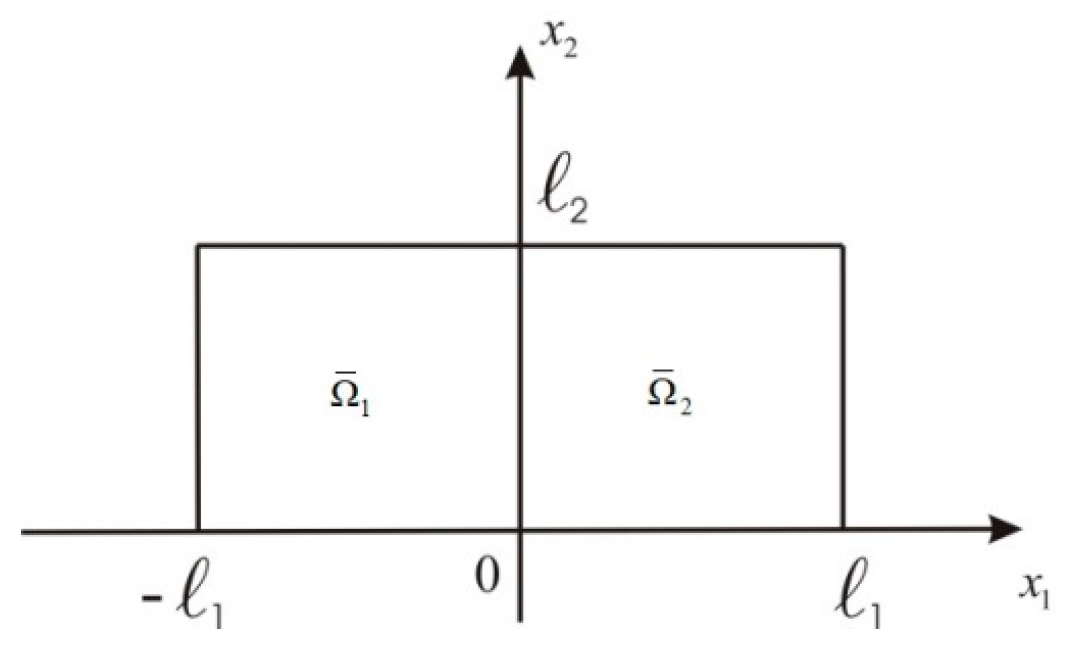
For instance, let us consider ${\mathrm{k}}_0=2$, i.e., two plates with different properties occupying the rectangular region $\overline{\mathrm{\Omega }}={\overline{\mathrm{\Omega }}}_1\cup {\overline{\mathrm{\Omega }}}_2=\left\{\mathrm{x}=\left({\mathrm{x}}_1,{\mathrm{x}}_2\right)| -{\ell }_1\le {\mathrm{x}}_1\le {\ell }_1, 0\le {\mathrm{x}}_2\le {\ell }_2\right\}$ (Figure 1).

In the case that the plates are connected through with a beam whose bending stiffness coefficients are ${\mathrm{B}}_{\mathrm{k}}$ and torsional stiffness coefficients are ${\mathrm{C}}_{\mathrm{k}}$ on the common boundary ${\mathrm{x}}_1=0$, the potential energy of the plate system is [21]

$$\begin{array}{l}\mathrm{I}\left(\mathsf{\omega }\right)=\frac{1}{2}{\displaystyle \sum _{\mathrm{k}=1}^2\{{\left(-1\right)}^{\mathrm{k}}{\displaystyle \underset{0}{\overset{{\ell }_1}{\int }}{\displaystyle \underset{0}{\overset{{\ell }_2}{\int }}{\mathrm{D}}_{\mathrm{k}}\left[{\left(\frac{{\partial }^2\mathsf{\omega }}{\partial {\mathrm{x}}_1^2}\right)}^2+{\left(\frac{{\partial }^2\mathsf{\omega }}{\partial {\mathrm{x}}_2^2}\right)}^2+2{\mathsf{\nu }}_{\mathrm{k}}\frac{{\partial }^2\mathsf{\omega }}{\partial {\mathrm{x}}_1^2}\frac{{\partial }^2\mathsf{\omega }}{\partial {\mathrm{x}}_2^2}+2\left(1-{\mathsf{\nu }}_{\mathrm{k}}\right){\left(\frac{{\partial }^2\mathsf{\omega }}{\partial {\mathrm{x}}_1\partial {\mathrm{x}}_2}\right)}^2\right]\mathrm{d}{\mathrm{x}}_2\mathrm{d}{\mathrm{x}}_1}}}\\ +{\displaystyle \underset{0}{\overset{{\mathrm{l}}_2}{\int }}{\left[{\mathrm{B}}_{\mathrm{k}}{\left(\frac{{\partial }^2\mathsf{\omega }}{\partial {\mathrm{x}}_2^2}\right)}^2+{\mathrm{C}}_{\mathrm{k}}{\left(\frac{{\partial }^2\mathsf{\omega }}{\partial {\mathrm{x}}_1^{}\partial {\mathrm{x}}_2^{}}\right)}^2\right]}_{{\mathrm{x}}_1=0}}\mathrm{d}{\mathrm{x}}_2\}+\frac{1}{2}{\displaystyle \underset{0}{\overset{{\mathrm{l}}_2}{\int }}{\left[\mathsf{\alpha }{\left(\frac{{\partial }^2\mathsf{\omega }}{\partial {\mathrm{x}}_1^2}\right)}^2+\mathsf{\beta } {\mathsf{\omega }}^2\right]}_{{\mathrm{x}}_1=0}}\mathrm{d}{\mathrm{x}}_2-\underset{0}{\overset{{\ell }_2}{\int }}\underset{-{\ell }_1}{\overset{{\ell }_1}{\int }}{\mathrm{q} (\mathrm{x}}_1{,\mathrm{x}}_2)\mathsf{\omega }{\mathrm{dx}}_1{\mathrm{dx}}_2.\end{array}$$

(2)

Here, $\mathsf{\alpha }$ is the stiffness coefficient of the hinge of the connected plates, while $\mathsf{\beta }$ is the stiffness coefficient of support (anchorage provided by the hinge). For the loaded elastic body to reach equilibrium, the Gateaux derivative of the full potential energy of the plates must be equal to zero.

$$\begin{array}{l}\mathsf{\delta }\mathrm{I}\left(\mathsf{\omega }\right)={\frac{\mathrm{d}}{\mathrm{dt}}\left[\mathrm{I}\left(\mathsf{\omega }+\mathrm{t}\mathsf{\vartheta }\right)\right]|}_{\mathrm{t}=0}\\ =\frac{\mathrm{d}}{\mathrm{dt}}\{{\displaystyle \sum _{\mathrm{k}=1}^2{\left(-1\right)}^{\mathrm{k}}\{\frac{1}{2}\underset{0}{\overset{{\ell }_2}{\int }}\underset{0}{\overset{{\ell }_1}{\int }}{\mathrm{D}}_{\mathrm{k}}\left\{{\left(\mathsf{\Delta }\left(\mathsf{\omega }+\mathrm{t}\mathsf{\vartheta }\right)\right)}^2-2\left(1-{\mathsf{\nu }}_{\mathrm{k}}\right)\left[\frac{{\partial }^2\left(\mathsf{\omega }+\mathrm{t}\mathsf{\vartheta }\right)}{\partial {\mathrm{x}}_1^2}\frac{{\partial }^2\left(\mathsf{\omega }+\mathrm{t}\mathsf{\vartheta }\right)}{\partial {\mathrm{x}}_2^2}-\frac{{\partial }^2\left(\mathsf{\omega }+\mathrm{t}\mathsf{\vartheta }\right)}{\partial {\mathrm{x}}_1\partial {\mathrm{x}}_2}\right]\right\}{\mathrm{dx}}_1{\mathrm{dx}}_2}\\ +\frac{1}{2}\underset{0}{\overset{{\ell }_2}{\int }}{\left[{\mathrm{B}}_{\mathrm{k}}{\left(\frac{{\partial }^2\left(\mathsf{\omega }+\mathrm{t}\mathsf{\vartheta }\right)}{\partial {\mathrm{x}}_2^2}\right)}^2+{\mathrm{C}}_{\mathrm{k}}{\left(\frac{{\partial }^2\left(\mathsf{\omega }+\mathrm{t}\mathsf{\vartheta }\right)}{\partial {\mathrm{x}}_1\partial {\mathrm{x}}_2}\right)}^2\right]}_{{\mathrm{x}}_1=0}{\mathrm{dx}}_2\}\\ {+\frac{1}{2}\underset{0}{\overset{{\ell }_2}{\int }}{\left\{\mathsf{\alpha }\left[{\left(\frac{{\partial }^2\left(\mathsf{\omega }+\mathrm{t}\mathsf{\vartheta }\right)}{\partial {\mathrm{x}}_1^2}\right)}^2+\mathsf{\beta }{\left(\mathsf{\omega }+\mathrm{t}\mathsf{\vartheta }\right)}^2\right]\right\}}_{{\mathrm{x}}_1=0}{\mathrm{dx}}_2-\underset{0}{\overset{{\ell }_2}{\int }}\underset{-{\ell }_1}{\overset{{\ell }_1}{\int }}\mathrm{q}\left(\mathrm{x}\right){\mathsf{\omega }\mathrm{dx}}_1{\mathrm{dx}}_2\}}_{\mathrm{t}=0}\\ =\{{\displaystyle \sum _{\mathrm{k}=1}^2{\left(-1\right)}^{\mathrm{k}}\{\frac{1}{2}\underset{0}{\overset{{\ell }_2}{\int }}\underset{0}{\overset{{\ell }_1}{\int }}{\mathrm{D}}_{\mathrm{k}}\{2\left(\frac{{\partial }^2\left(\mathsf{\omega }+\mathrm{t}\mathsf{\vartheta }\right)}{\partial {\mathrm{x}}_1^2}+\frac{{\partial }^2\left(\mathsf{\omega }+\mathrm{t}\mathsf{\vartheta }\right)}{\partial {\mathrm{x}}_2^2}\right)\left(\frac{{\partial }^2\mathsf{\vartheta }}{\partial {\mathrm{x}}_1^2}+\frac{{\partial }^2\mathsf{\vartheta }}{\partial {\mathrm{x}}_2^2}\right)}\\ -2\left(1-{\mathsf{\nu }}_{\mathrm{k}}\right)\left[\frac{{\partial }^2\mathsf{\vartheta }}{\partial {\mathrm{x}}_1^2}\frac{{\partial }^2\left(\mathsf{\omega }+\mathrm{t}\mathsf{\vartheta }\right)}{\partial {\mathrm{x}}_2^2}+\frac{{\partial }^2\left(\mathsf{\omega }+\mathrm{t}\mathsf{\vartheta }\right)}{\partial {\mathrm{x}}_1^2}\frac{{\partial }^2\mathsf{\vartheta }}{\partial {\mathrm{x}}_2^2}-2\frac{{\partial }^2\left(\mathsf{\omega }+\mathrm{t}\mathsf{\vartheta }\right)}{\partial {\mathrm{x}}_1\partial {\mathrm{x}}_2}\frac{{\partial }^2\mathsf{\vartheta }}{\partial {\mathrm{x}}_1\partial {\mathrm{x}}_2}\right]\}{\mathrm{dx}}_1{\mathrm{dx}}_2\\ +\frac{1}{2}\underset{0}{\overset{{\ell }_2}{\int }}{\left[2{\mathrm{B}}_{\mathrm{k}}\frac{{\partial }^2\left(\mathsf{\omega }+\mathrm{t}\mathsf{\vartheta }\right)}{\partial {\mathrm{x}}_2^2}\frac{{\partial }^2\mathsf{\vartheta }}{\partial {\mathrm{x}}_2^2}+2{\mathrm{C}}_{\mathrm{k}}\frac{{\partial }^2\left(\mathsf{\omega }+\mathrm{t}\mathsf{\vartheta }\right)}{\partial {\mathrm{x}}_1\partial {\mathrm{x}}_2}\frac{{\partial }^2\mathsf{\vartheta }}{\partial {\mathrm{x}}_1\partial {\mathrm{x}}_2}\right]|}_{{\mathrm{x}}_1=0}{\mathrm{dx}}_2\}\\ {+\frac{1}{2}\underset{0}{\overset{{\ell }_2}{\int }}{\left[2\mathsf{\alpha }\frac{\partial \left(\mathsf{\omega }+\mathrm{t}\mathsf{\vartheta }\right)}{\partial {\mathrm{x}}_1}\frac{\partial \mathsf{\vartheta }}{\partial {\mathrm{x}}_1}+2\mathsf{\beta }\left(\mathsf{\omega }+\mathrm{t}\mathsf{\vartheta }\right)\mathsf{\vartheta }\right]|}_{{\mathrm{x}}_1=0}{\mathrm{dx}}_2-\underset{0}{\overset{{\ell }_2}{\int }}\underset{-{\ell }_1}{\overset{{\ell }_1}{\int }}\mathrm{q}\left(\mathrm{x}\right)\mathsf{\vartheta }{\mathrm{dx}}_1{\mathrm{dx}}_2\}|}_{\mathrm{t}=0}\\ ={\displaystyle \sum _{\mathrm{k}=1}^2{\left(-1\right)}^{\mathrm{k}}\{\underset{0}{\overset{{\ell }_2}{\int }}\underset{0}{\overset{{\ell }_1}{\int }}{\mathrm{D}}_{\mathrm{k}}\{\left(\frac{{\partial }^2\mathsf{\omega }}{\partial {\mathrm{x}}_1^2}+\frac{{\partial }^2\mathsf{\omega }}{\partial {\mathrm{x}}_2^2}\right)\left(\frac{{\partial }^2\mathsf{\vartheta }}{\partial {\mathrm{x}}_1^2}+\frac{{\partial }^2\mathsf{\vartheta }}{\partial {\mathrm{x}}_2^2}\right)}\\ -\left(1-{\mathsf{\nu }}_{\mathrm{k}}\right)\left[\frac{{\partial }^2\mathsf{\vartheta }}{\partial {\mathrm{x}}_1^2}\frac{{\partial }^2\mathsf{\omega }}{\partial {\mathrm{x}}_2^2}+\frac{{\partial }^2\mathsf{\omega }}{\partial {\mathrm{x}}_1^2}\frac{{\partial }^2\mathsf{\vartheta }}{\partial {\mathrm{x}}_2^2}-2\frac{{\partial }^2\mathsf{\omega }}{\partial {\mathrm{x}}_1\partial {\mathrm{x}}_2}\frac{{\partial }^2\mathsf{\vartheta }}{\partial {\mathrm{x}}_1\partial {\mathrm{x}}_2}\right]\}{\mathrm{dx}}_1{\mathrm{dx}}_2\\ +\underset{0}{\overset{{\ell }_2}{\int }}{\left[{\mathrm{B}}_{\mathrm{k}}\frac{{\partial }^2\mathsf{\omega }}{\partial {\mathrm{x}}_2^2}\frac{{\partial }^2\mathsf{\vartheta }}{\partial {\mathrm{x}}_2^2}+{\mathrm{C}}_{\mathrm{k}}\frac{{\partial }^2\mathsf{\omega }}{\partial {\mathrm{x}}_1\partial {\mathrm{x}}_2}\frac{{\partial }^2\mathsf{\vartheta }}{\partial {\mathrm{x}}_1\partial {\mathrm{x}}_2}\right]|}_{{\mathrm{x}}_1=0}{\mathrm{dx}}_2\}+\underset{0}{\overset{{\ell }_2}{\int }}{\left[\mathsf{\alpha }\frac{\partial \mathsf{\omega }}{\partial {\mathrm{x}}_1}\frac{\partial \mathsf{\vartheta }}{\partial {\mathrm{x}}_1}+\mathsf{\beta }\mathsf{\omega }\mathsf{\vartheta }\right]|}_{{\mathrm{x}}_1=0}{\mathrm{dx}}_2-\underset{0}{\overset{{\ell }_2}{\int }}\underset{-{\ell }_1}{\overset{{\ell }_1}{\int }}\mathrm{q}\left(\mathrm{x}\right)\mathsf{\vartheta }{\mathrm{dx}}_1{\mathrm{dx}}_2,\end{array}$$

where $\mathrm{t}\in \mathrm{R}$ and the function $\mathsf{\vartheta }$ is in the same class as the function $\mathsf{\omega }$. Thus, we obtain

$$\begin{array}{l}\mathsf{\delta }\mathrm{I}\left(\mathsf{\omega }\right) ={\displaystyle \sum _{\mathrm{k}=1}^2\{{\left(-1\right)}^{\mathrm{k}}{\displaystyle \underset{0}{\overset{{\ell }_2}{\int }}{\displaystyle \underset{0}{\overset{{\ell }_1}{\int }}{\mathrm{D}}_{\mathrm{k}}[\frac{{\partial }^2\mathsf{\vartheta }}{\partial {\mathrm{x}}_1^2}\left(\frac{{\partial }^2\mathsf{\omega }}{\partial {\mathrm{x}}_1^2}+{\mathsf{\nu }}_{\mathrm{k}}\frac{{\partial }^2\mathsf{\omega }}{\partial {\mathrm{x}}_2^2}\right)+\frac{{\partial }^2\mathsf{\vartheta }}{\partial {\mathrm{x}}_2^2}\left(\frac{{\partial }^2\mathsf{\omega }}{\partial {\mathrm{x}}_2^2}+{\mathsf{\nu }}_{\mathrm{k}}\frac{{\partial }^2\mathsf{\omega }}{\partial {\mathrm{x}}_1^2}\right)}}}\\ +2\left(1-{\mathsf{\nu }}_{\mathrm{k}}\right)\frac{{\partial }^2\mathsf{\omega }}{\partial {\mathrm{x}}_1\partial {\mathrm{x}}_2}\frac{{\partial }^2\mathsf{\vartheta }}{\partial {\mathrm{x}}_1\partial {\mathrm{x}}_2}]{\mathrm{dx}}_1{\mathrm{dx}}_2+\underset{0}{\overset{{\ell }_2}{\int }}{\left[{\mathrm{B}}_{\mathrm{k}}\frac{{\partial }^2\mathsf{\omega }}{\partial {\mathrm{x}}_2^2}\frac{{\partial }^2\mathsf{\vartheta }}{\partial {\mathrm{x}}_2^2}+{\mathrm{C}}_{\mathrm{k}}\frac{{\partial }^2\mathsf{\omega }}{\partial {\mathrm{x}}_1\partial {\mathrm{x}}_2}\frac{{\partial }^2\mathsf{\vartheta }}{\partial {\mathrm{x}}_1\partial {\mathrm{x}}_2}\right]|}_{{\mathrm{x}}_1=0}{\mathrm{dx}}_2\}\\ +\underset{0}{\overset{{\ell }_2}{\int }}{\left[\mathsf{\alpha }\frac{\partial \mathsf{\omega }}{\partial {\mathrm{x}}_1}\frac{\partial \mathsf{\vartheta }}{\partial {\mathrm{x}}_1}+\mathsf{\beta }\mathsf{\omega }\mathsf{\vartheta }\right]|}_{{\mathrm{x}}_1=0}{\mathrm{dx}}_2-\underset{0}{\overset{{\ell }_2}{\int }}\underset{-{\ell }_1}{\overset{{\ell }_1}{\int }}\mathrm{q}\left(\mathrm{x}\right)\mathsf{\vartheta }{\mathrm{dx}}_1{\mathrm{dx}}_2=0.\end{array}$$

(3)

After calculating the integrals in (3), the terms corresponding to the common boundary ${\mathrm{x}}_1=0$ of the plates are written down as follows:

$$\begin{array}{l}\underset{0}{\overset{{\ell }_2}{\int }}\{[-{\mathrm{D}}_2\left(\frac{{\partial }^2\mathsf{\omega }}{\partial {\mathrm{x}}_1^2}+{\mathsf{\nu }}_2\frac{{\partial }^2\mathsf{\omega }}{\partial {\mathrm{x}}_2^2}\right)\frac{\partial \mathsf{\vartheta }}{\partial {\mathrm{x}}_1}+\frac{\partial }{\partial {\mathrm{x}}_1}\left[{\mathrm{D}}_2\left(\frac{{\partial }^2\mathsf{\omega }}{\partial {\mathrm{x}}_1^2}+{\mathsf{\nu }}_2\frac{{\partial }^2\mathsf{\omega }}{\partial {\mathrm{x}}_2^2}\right)\right]\mathsf{\vartheta }+2\frac{\partial }{\partial {\mathrm{x}}_2}\left[{\mathrm{D}}_2\left(1-{\mathsf{\nu }}_2\right)\frac{{\partial }^2\mathsf{\omega }}{\partial {\mathrm{x}}_1\partial {\mathrm{x}}_2}\right]\mathsf{\vartheta }\\ {+\frac{{\partial }^2}{\partial {\mathrm{x}}_2^2}\left({\mathrm{B}}_2\frac{{\partial }^2\mathsf{\omega }}{\partial {\mathrm{x}}_2^2}\right)\mathsf{\vartheta }-\frac{\partial }{\partial {\mathrm{x}}_2}\left({\mathrm{C}}_2\frac{{\partial }^2\mathsf{\omega }}{\partial {\mathrm{x}}_1\partial {\mathrm{x}}_2}\right)\frac{\partial \mathsf{\vartheta }}{\partial {\mathrm{x}}_1}]|}_{{\mathrm{x}}_1=0^{+}}+[{\mathrm{D}}_1\left(\frac{{\partial }^2\mathsf{\omega }}{\partial {\mathrm{x}}_1^2}+{\mathsf{\nu }}_1\frac{{\partial }^2\mathsf{\omega }}{\partial {\mathrm{x}}_2^2}\right)\frac{\partial \mathsf{\vartheta }}{\partial {\mathrm{x}}_1}-\frac{\partial }{\partial {\mathrm{x}}_1}\left[{\mathrm{D}}_1\left(\frac{{\partial }^2\mathsf{\omega }}{\partial {\mathrm{x}}_1^2}+{\mathsf{\nu }}_1\frac{{\partial }^2\mathsf{\omega }}{\partial {\mathrm{x}}_2^2}\right)\right]\mathsf{\vartheta }\\ {-2\frac{\partial }{\partial {\mathrm{x}}_2}\left[{\mathrm{D}}_1\left(1-{\mathsf{\nu }}_1\right)\frac{{\partial }^2\mathsf{\omega }}{\partial {\mathrm{x}}_1\partial {\mathrm{x}}_2}\right]\mathsf{\vartheta }+\frac{{\partial }^2}{\partial {\mathrm{x}}_2^2}\left({\mathrm{B}}_1\frac{{\partial }^2\mathsf{\omega }}{\partial {\mathrm{x}}_2^2}\right)\mathsf{\vartheta }-\frac{\partial }{\partial {\mathrm{x}}_2}\left({\mathrm{C}}_1\frac{{\partial }^2\mathsf{\omega }}{\partial {\mathrm{x}}_1\partial {\mathrm{x}}_2}\right)\frac{\partial \mathsf{\vartheta }}{\partial {\mathrm{x}}_1}]|}_{{\mathrm{x}}_1=0^{-}}\\ +\mathsf{\alpha }\left[{\frac{\partial \mathsf{\omega }}{\partial {\mathrm{x}}_1}|}_{{\mathrm{x}}_1=0^{+}}-{\frac{\partial \mathsf{\omega }}{\partial {\mathrm{x}}_1}|}_{{\mathrm{x}}_1=0^{-}}\right]\left[{\frac{\partial \mathsf{\vartheta }}{\partial {\mathrm{x}}_1}|}_{{\mathrm{x}}_1=0^{+}}-{\frac{\partial \mathsf{\vartheta }}{\partial {\mathrm{x}}_1}|}_{{\mathrm{x}}_1=0^{-}}\right]{+\mathsf{\beta }\mathsf{\omega }\mathsf{\vartheta }|}_{{\mathrm{x}}_1=0}\}{\mathrm{dx}}_2.\end{array}$$

Obtaining the transmission conditions on the common boundary ${\mathrm{x}}_1=0$ of the plates firstly involves writing down the terms corresponding to this edge where the coefficients of $\mathsf{\vartheta }, {\frac{\partial \mathsf{\vartheta }}{\partial {\mathrm{x}}_1}|}_{{\mathrm{x}}_1=0^{+}}, {\frac{\partial \mathsf{\vartheta }}{\partial {\mathrm{x}}_1}|}_{{\mathrm{x}}_1=0^{-}}$ expressions are equal to zero, and then the discontinuity of ω is also added on the common border, and the following transmission conditions are obtained:

$$\mathsf{\alpha }⟦\frac{\partial \mathsf{\omega }}{\partial {\mathrm{x}}_1}⟧=\frac{1}{2}\{{\mathrm{D}}_2{\left(\frac{{\partial }^2\mathsf{\omega }}{\partial {\mathrm{x}}_1^2}+{\mathsf{\nu }}_2\frac{{\partial }^2\mathsf{\omega }}{\partial {\mathrm{x}}_2^2}\right)}_{{\mathrm{x}}_1=0^{+}}+{\mathrm{D}}_1{\left(\frac{{\partial }^2\mathsf{\omega }}{\partial {\mathrm{x}}_1^2}+{\mathsf{\nu }}_1\frac{{\partial }^2\mathsf{\omega }}{\partial {\mathrm{x}}_2^2}\right)}_{{\mathrm{x}}_1=0^{-}}+\frac{\partial }{\partial {\mathrm{x}}_2}{\left({\mathrm{C}}_2\frac{{\partial }^2\mathsf{\omega }}{\partial {\mathrm{x}}_1\partial {\mathrm{x}}_2}\right)}_{{\mathrm{x}}_1=0^{+}}-\frac{\partial }{\partial {\mathrm{x}}_2}{\left({\mathrm{C}}_1\frac{{\partial }^2\mathsf{\omega }}{\partial {\mathrm{x}}_1\partial {\mathrm{x}}_2}\right)}_{{\mathrm{x}}_1=0^{-}}\},$$

(4)

$$\left({\mathrm{D}}_2{\left(\frac{{\partial }^2\mathsf{\omega }}{\partial {\mathrm{x}}_1^2}+{\mathsf{\nu }}_2\frac{{\partial }^2\mathsf{\omega }}{\partial {\mathrm{x}}_2^2}\right)}_{{\mathrm{x}}_1=0^{+}}-{\mathrm{D}}_1{\left(\frac{{\partial }^2\mathsf{\omega }}{\partial {\mathrm{x}}_1^2}+{\mathsf{\nu }}_1\frac{{\partial }^2\mathsf{\omega }}{\partial {\mathrm{x}}_2^2}\right)}_{{\mathrm{x}}_1=0^{-}}\right)=-\left\{\frac{\partial }{\partial {\mathrm{x}}_2}{\left({\mathrm{C}}_2\frac{{\partial }^2\mathsf{\omega }}{\partial {\mathrm{x}}_1\partial {\mathrm{x}}_2}\right)}_{{\mathrm{x}}_1=0^{+}}+\frac{\partial }{\partial {\mathrm{x}}_2}{\left({\mathrm{C}}_1\frac{{\partial }^2\mathsf{\omega }}{\partial {\mathrm{x}}_1\partial {\mathrm{x}}_2}\right)}_{{\mathrm{x}}_1=0^{-}}\right\},$$

(5)

$$\begin{array}{l}\{{\left(\frac{\partial }{\partial {\mathrm{x}}_1}\left[{\mathrm{D}}_2\left(\frac{{\partial }^2\mathsf{\omega }}{\partial {\mathrm{x}}_1^2}+{\mathsf{\nu }}_2\frac{{\partial }^2\mathsf{\omega }}{\partial {\mathrm{x}}_2^2}\right)\right]+2\frac{\partial }{\partial {\mathrm{x}}_2}\left[{\mathrm{D}}_2\left(1-{\mathsf{\nu }}_2\right)\frac{{\partial }^2\mathsf{\omega }}{\partial {\mathrm{x}}_1\partial {\mathrm{x}}_2}\right]\right)}_{{\mathrm{x}}_1=0^{+}}\\ \hspace{1em}-{\left(\frac{\partial }{\partial {\mathrm{x}}_1}\left[{\mathrm{D}}_1\left(\frac{{\partial }^2\mathsf{\omega }}{\partial {\mathrm{x}}_1^2}+{\mathsf{\nu }}_1\frac{{\partial }^2\mathsf{\omega }}{\partial {\mathrm{x}}_2^2}\right)\right]+2\frac{\partial }{\partial {\mathrm{x}}_2}\left[{\mathrm{D}}_1\left(1-{\mathsf{\nu }}_1\right)\frac{{\partial }^2\mathsf{\omega }}{\partial {\mathrm{x}}_1\partial {\mathrm{x}}_2}\right]\right)}_{{\mathrm{x}}_1=0^{-}}\}={\left(-\mathsf{\beta }\mathsf{\omega }-\frac{{\partial }^2}{\partial {\mathrm{x}}_2^2}\left({\mathrm{B}}_1+{\mathrm{B}}_2\right)\frac{{\partial }^2\mathsf{\omega }}{\partial {\mathrm{x}}_2^2}\right)}_{{\mathrm{x}}_1=0}.\end{array}$$

(6)

Here, $⟦\frac{\partial \mathsf{\omega }}{\partial {\mathrm{x}}_1}⟧$ is known as the jump of $\frac{\partial \mathsf{\omega }}{\partial {\mathrm{x}}_1}$ at ${\mathrm{x}}_1=0$. Usually, based on the shape of the junction of the plates on the common boundary, there are different meanings of transmission conditions depending on different values of non-negative constants $\mathsf{\alpha }, \mathsf{\beta }$, and ${\mathrm{B}}_{\mathrm{k}},{\mathrm{C}}_{\mathrm{k}}, \mathrm{k}=1,2$.

4. The Finite Difference Approximations of the Transmission Conditions

Let us define the mesh ${\overline{\mathrm{\Omega }}}_{{\mathrm{h}}_1{\mathrm{h}}_2}={\overline{\mathrm{\Omega }}}_{{\mathrm{h}}_1}\times {\overline{\mathrm{\Omega }}}_{{\mathrm{h}}_2}=\left\{({\mathrm{x}}_1^{\mathrm{i}},{\mathrm{x}}_2^{\mathrm{j}}) | {\mathrm{x}}_1^{\mathrm{i}}\in {\overline{\mathrm{\Omega }}}_{{\mathrm{h}}_1},{\mathrm{x}}_2^{\mathrm{j}}\in {\overline{\mathrm{\Omega }}}_{{\mathrm{h}}_2} ,\mathrm{i}=\overline{1,\mathrm{n}}, \mathrm{j}=\overline{1,\mathrm{m}}\right\}$ sized $\mathrm{n}\mathrm{x}\mathrm{m}$ in the region $\mathrm{\Omega }\subset {\mathrm{R}}^2$, where ${\overline{\mathrm{\Omega }}}_{{\mathrm{h}}_1}$, ${\overline{\mathrm{\Omega }}}_{{\mathrm{h}}_2}$ are the uniform meshes on the axes ${\mathrm{x}}_1, {\mathrm{x}}_2$, respectively (also ${\mathrm{h}}_1, {\mathrm{h}}_2$ are step widths of meshes, $\mathrm{n}, \mathrm{m}$ are the number of points on the axes ${\mathrm{x}}_1, {\mathrm{x}}_2$, respectively). In order to obtain the finite difference equations that correspond to the problem described in a previous study [21], let us use the functional approximation method. Considering the expressions of the transmission conditions (4)–(6) and $\mathsf{\alpha }\ne 0$,${\mathrm{C}}_{\mathrm{k}}=0, {\mathrm{B}}_{\mathrm{k}}=\mathrm{B}, \mathrm{k}=1,2$, we may show the finite difference approximation of the functional $\mathrm{i}\left(\mathsf{\omega }\right)$ as

$${\mathrm{I}}_{\mathrm{h}}\left(\mathrm{y}\right)={\displaystyle \sum _{\mathrm{k}=1}^2{\mathrm{W}}_{\mathrm{h}}^{\mathrm{k}}\left(\mathrm{y}\right)}+{\mathrm{W}}_{\mathrm{h}}^{\mathsf{\gamma }}\left(\mathrm{y}\right)-\sum _{{\overline{\mathrm{\Omega }}}_{{\mathrm{h}}_1{\mathrm{h}}_2}}{\mathrm{qyh}}_1{\mathrm{h}}_2.$$

Here, ${\mathrm{W}}_{\mathrm{h}}^{\mathrm{k}}\left(\mathrm{y}\right), \mathrm{k}=1,2$ are the finite difference approximations of the energy functions on meshes ${\overline{\mathrm{\Omega }}}_{{\mathrm{h}}_1{\mathrm{h}}_2}$. Additionally, ${\mathrm{W}}_{\mathrm{h}}^{\mathsf{\gamma }}\left(\mathrm{y}\right)$ are the finite difference expressions of the collected terms that belong to the common boundary $\mathsf{\gamma }$. The expression ${\mathrm{W}}_{\mathrm{h}}^{\mathsf{\gamma }}\left(\mathrm{y}\right)$ is obtained as follows:

$$\begin{array}{l}{\mathrm{W}}_{\mathrm{h}}^{\mathsf{\gamma }}\left(\mathrm{y}\right)=\frac{{\mathrm{h}}_1}{2}{\displaystyle \sum _{\mathsf{\gamma }}{\mathrm{h}}_2\{2\tilde{\mathrm{D}}{\left({\mathrm{y}}_{\overline{{\mathrm{x}}_1}{\mathrm{x}}_1}\right)}^2+[\frac{\mathrm{B}}{{\mathrm{h}}_1}+\frac{1}{2}\left[{\mathrm{D}}_1\left(1-{\left({\mathsf{\nu }}_1\right)}^2\right)+{\mathrm{D}}_2\left(1-{\left({\mathsf{\nu }}_2\right)}^2\right)\right]+\frac{{\left({\mathsf{\nu }}_1+{\mathsf{\nu }}_2\right)}^2}{2}\tilde{\mathrm{D}}]{\left({\mathrm{y}}_{\overline{{\mathrm{x}}_2}{\mathrm{x}}_2}\right)}^2}\\ \hspace{1em}\hspace{1em}\hspace{1em}\hspace{1em}+2\left({\mathsf{\nu }}_1+{\mathsf{\nu }}_2\right)\tilde{\mathrm{D}}{\mathrm{y}}_{\overline{{\mathrm{x}}_1}{\mathrm{x}}_1}{\mathrm{y}}_{\overline{{\mathrm{x}}_2}{\mathrm{x}}_2}+\frac{\mathsf{\beta }}{{\mathrm{h}}_1}{\mathrm{y}}^2\}\end{array},$$

(7)

where $\tilde{\mathrm{D}}=2\mathsf{\alpha }{\mathrm{h}}_1{\mathrm{D}}_1{\mathrm{D}}_2/\left(2{\mathrm{D}}_1{\mathrm{D}}_2+\mathsf{\alpha }{\mathrm{h}}_1\left({\mathrm{D}}_1+{\mathrm{D}}_2\right)\right)$, ${\mathrm{y}}_{\overline{{\mathrm{x}}_1}}, {\mathrm{y}}_{\overline{{\mathrm{x}}_2}}$ denote the left-hand derivatives and ${\mathrm{y}}_{{\mathrm{x}}_1}, {\mathrm{y}}_{{\mathrm{x}}_2}$ denote the right-hand derivatives of function $\mathrm{y}$ on the axes ${\mathrm{x}}_1, {\mathrm{x}}_2$, respectively. Defining the following coefficients,

$${\mathrm{D}}_1=\{\begin{array}{lll}{\mathrm{D}}_1& ,& \mathrm{x}=\left(-{\mathrm{h}}_1,{\mathrm{x}}_2\right)\\ 2\tilde{\mathrm{D}}& ,& \mathrm{x}=\left(0,{\mathrm{x}}_2\right)\\ {\mathrm{D}}_2& ,& \mathrm{x}=\left({\mathrm{h}}_1,{\mathrm{x}}_2\right)\end{array},$$

(8)

$${\mathrm{D}}_2=\{\begin{array}{lll}{\mathrm{D}}_1& ,& \mathrm{x}=\left(-{\mathrm{h}}_1,{\mathrm{x}}_2\right)\\ \frac{\mathrm{B}}{{\mathrm{h}}_1}+\frac{1}{2}\left[{\mathrm{D}}_1\left(1-{\left({\mathsf{\nu }}_1\right)}^2\right)+{\mathrm{D}}_2\left(1-{\left({\mathsf{\nu }}_2\right)}^2\right)\right]+\frac{{\left({\mathsf{\nu }}_1+{\mathsf{\nu }}_2\right)}^2}{2}\tilde{\mathrm{D}}& ,& \mathrm{x}=\left(0,{\mathrm{x}}_2\right)\\ {\mathrm{D}}_2& ,& \mathrm{x}=\left({\mathrm{h}}_1,{\mathrm{x}}_2\right)\end{array},$$

(9)

$${\mathrm{D}}_{\mathrm{kp}}=\frac{{\mathrm{D}}_1\left(1-{\mathsf{\nu }}_1\right)+{\mathrm{D}}_2\left(1-{\mathsf{\nu }}_2\right)}{4},$$

(10)

we may rewrite ${\mathrm{I}}_{\mathrm{h}}\left(\mathrm{y}\right)$ by using (8)–(10) as follows:

$$\begin{array}{l}{\mathrm{I}}_{\mathrm{h}}\left(\mathrm{y}\right)=\frac{{\mathrm{h}}_1{\mathrm{h}}_2}{2}{\displaystyle \sum _{{\mathrm{\Omega }}_{{\mathrm{h}}_1{\mathrm{h}}_2}}\{{\mathrm{D}}_1{\left({\mathrm{y}}_{\overline{{\mathrm{x}}_1}{\mathrm{x}}_1}\right)}^2+{\mathrm{D}}_2{\left({\mathrm{y}}_{\overline{{\mathrm{x}}_2}{\mathrm{x}}_2}\right)}^2+{\mathrm{D}}_1\left({\mathsf{\nu }}_1+{\mathsf{\nu }}_2\right){\mathrm{y}}_{\overline{{\mathrm{x}}_1}{\mathrm{x}}_1}{\mathrm{y}}_{\overline{{\mathrm{x}}_2}{\mathrm{x}}_2}} \\ \hspace{1em}\hspace{1em}\hspace{1em}+{\mathrm{D}}_{\mathrm{k}\mathrm{p}}\left[{\left({\mathrm{y}}_{\overline{{\mathrm{x}}_1}\overline{{\mathrm{x}}_2}}\right)}^2+{\left({\mathrm{y}}_{{\mathrm{x}}_1\overline{{\mathrm{x}}_2}}\right)}^2+{\left({\mathrm{y}}_{\overline{{\mathrm{x}}_1}{\mathrm{x}}_2}\right)}^2+{\left({\mathrm{y}}_{{\mathrm{x}}_1{\mathrm{x}}_2}\right)}^2\right]+\mathsf{\beta }\mathsf{\delta }\left({\mathrm{x}}_1\right){\mathrm{y}}^2-2\mathrm{qy}\},\end{array}$$

(11)

where the Dirac function is

$$\mathsf{\delta }\left({\mathrm{x}}_1\right)= \{\begin{array}{c}1/{\mathrm{h}}_1, {\mathrm{x}}_1=0 \\ 0, {\mathrm{x}}_1\ne 0.\end{array}$$

(12)

The ${\mathrm{I}}_{\mathrm{h}}\left(\mathrm{y}\right)$ that was obtained above is a multivariable function that depends on the variables ${\mathrm{y}}_{\mathrm{i}\mathrm{j}}=\mathrm{y}({\mathrm{x}}_1^{\mathrm{i}},{\mathrm{x}}_2^{\mathrm{j}}),\hspace{1em}({\mathrm{x}}_1^{\mathrm{i}},{\mathrm{x}}_2^{\mathrm{j}})\in {\overline{\mathrm{\Omega }}}_{{\mathrm{h}}_1{\mathrm{h}}_2}$. Keeping this in consideration, if the derivative of the functional ${\mathrm{I}}_{\mathrm{h}}\left(\mathrm{y}\right)$ with respect to $\mathrm{y}\left({\mathrm{x}}_1,{\mathrm{x}}_2\right)$ is computed and equated to zero, we can obtain the finite difference expression of Equation (1) as the following:

$$\begin{array}{l}{\left({\mathrm{D}}_1{\mathrm{y}}_{\overline{{\mathrm{x}}_1}{\mathrm{x}}_1}\right)}_{\overline{{\mathrm{x}}_1}{\mathrm{x}}_1}+{\left({\mathrm{D}}_2{\mathrm{y}}_{\overline{{\mathrm{x}}_2}{\mathrm{x}}_2}\right)}_{\overline{{\mathrm{x}}_2}{\mathrm{x}}_2}+{\left({\mathrm{D}}_1\frac{\left({\mathsf{\nu }}_1+{\mathsf{\nu }}_2\right)}{2}{\mathrm{y}}_{\overline{{\mathrm{x}}_1}{\mathrm{x}}_1}\right)}_{\overline{{\mathrm{x}}_2}{\mathrm{x}}_2}\\ \hspace{1em}\hspace{1em}\hspace{1em}\hspace{1em}\hspace{1em}+{\left({\mathrm{D}}_1\frac{\left({\mathsf{\nu }}_1+{\mathsf{\nu }}_2\right)}{2}{\mathrm{y}}_{\overline{{\mathrm{x}}_2}{\mathrm{x}}_2}\right)}_{\overline{{\mathrm{x}}_1}{\mathrm{x}}_1}+4{\mathrm{D}}_{\mathrm{kp}}{\mathrm{y}}_{\overline{{\mathrm{x}}_1}{\mathrm{x}}_1\overline{{\mathrm{x}}_2}{\mathrm{x}}_2}+\mathsf{\beta }\mathsf{\delta }\left({\mathrm{x}}_1\right)\mathrm{y}=\mathrm{q}\left({\mathrm{x}}_1^{\mathrm{i}},{\mathrm{x}}_2^{\mathrm{j}}\right).\end{array}$$

(13)

Using Equation (13), we obtain the finite difference approximations of the transmission conditions on the points of the common border and their neighbors, i.e., ${\mathrm{x}}_1=0,\pm {\mathrm{h}}_1$. Firstly, Equation (13) is turned into (14) for the points $(-{\mathrm{h}}_1,{\mathrm{x}}_2^{\mathrm{j}}),\mathrm{j}=\overline{2,\mathrm{m}-1}$:

$$\begin{array}{l}{\mathrm{D}}_1\left\{{\mathrm{y}}_{\overline{{\mathrm{x}}_1}{\mathrm{x}}_1\overline{{\mathrm{x}}_1}{\mathrm{x}}_1}-\frac{1}{{\mathrm{h}}_1^2}{\mathrm{y}}_{{\mathrm{x}}_1{\mathrm{x}}_1}+{\mathrm{y}}_{\overline{{\mathrm{x}}_2}{\mathrm{x}}_2\overline{{\mathrm{x}}_2}{\mathrm{x}}_2}+\frac{\left({\mathsf{\nu }}_1+{\mathsf{\nu }}_2\right)}{2}\left(2{\mathrm{y}}_{\overline{{\mathrm{x}}_1}{\mathrm{x}}_1\overline{{\mathrm{x}}_2}{\mathrm{x}}_2}-\frac{1}{{\mathrm{h}}_1}{\mathrm{y}}_{{\mathrm{x}}_1\overline{{\mathrm{x}}_2}{\mathrm{x}}_2}-\frac{1}{{\mathrm{h}}_1^2}{\mathrm{y}}_{\overline{{\mathrm{x}}_2}{\mathrm{x}}_2}\right)\right\}\\ \hspace{1em}\hspace{1em}\hspace{1em}\hspace{1em}\hspace{1em}+\tilde{\mathrm{D}}\left\{\frac{\left({\mathsf{\nu }}_1+{\mathsf{\nu }}_2\right)}{2}\left[\frac{1}{{\mathrm{h}}_1^2}\left({\mathrm{y}}_{{\mathrm{x}}_1{\mathrm{x}}_1}+{\mathrm{y}}_{\overline{{\mathrm{x}}_2}{\mathrm{x}}_2}\right)+\frac{1}{{\mathrm{h}}_1}{\mathrm{y}}_{{\mathrm{x}}_1\overline{{\mathrm{x}}_2}{\mathrm{x}}_2}\right]+\frac{1}{{\mathrm{h}}_1^2}{\mathrm{y}}_{{\mathrm{x}}_1{\mathrm{x}}_1}\right\}\\ \hspace{1em}\hspace{1em}\hspace{1em}\hspace{1em}\hspace{1em}+\left[{\mathrm{D}}_1\left(1-{\mathrm{v}}_1\right)+{\mathrm{D}}_2\left(1-{\mathrm{v}}_2\right)\right]{\mathrm{y}}_{\overline{{\mathrm{x}}_1}{\mathrm{x}}_1\overline{{\mathrm{x}}_2}{\mathrm{x}}_2}=\mathrm{q}\left({-\mathrm{h}}_1,{\mathrm{x}}_2^{\mathrm{j}}\right).\end{array}$$

(14)

For the points that belong to the common border ${\mathrm{x}}_1=0$ in ${\overline{\mathrm{\Omega }}}_{{\mathrm{h}}_1{\mathrm{h}}_2}$, the finite difference expressions of the transmission conditions are

$$\begin{array}{l}2\tilde{\mathrm{D}}\{{\mathrm{y}}_{\overline{{\mathrm{x}}_1}{\mathrm{x}}_1\overline{{\mathrm{x}}_1}{\mathrm{x}}_1}+\frac{{\left({\mathsf{\nu }}_1+{\mathsf{\nu }}_2\right)}^2}{4}{\mathrm{y}}_{\overline{{\mathrm{x}}_2}{\mathrm{x}}_2\overline{{\mathrm{x}}_2}{\mathrm{x}}_2}-\frac{1}{{\mathrm{h}}_1^2}\left({\mathrm{y}}_{{\mathrm{x}}_1{\mathrm{x}}_1}+{\mathrm{y}}_{\overline{{\mathrm{x}}_1}\overline{{\mathrm{x}}_1}}\right)+\left({\mathsf{\nu }}_1+{\mathsf{\nu }}_2\right){\mathrm{y}}_{\overline{{\mathrm{x}}_1}{\mathrm{x}}_1\overline{{\mathrm{x}}_2}{\mathrm{x}}_2}\\ \hspace{1em}\hspace{1em}-\frac{\left({\mathsf{\nu }}_1+{\mathsf{\nu }}_2\right)}{2{\mathrm{h}}_1}\left({\mathrm{y}}_{{\mathrm{x}}_1\overline{{\mathrm{x}}_2}{\mathrm{x}}_2}-{\mathrm{y}}_{\overline{{\mathrm{x}}_1}\overline{{\mathrm{x}}_2}{\mathrm{x}}_2}\right)\}+\left\{\frac{\mathrm{B}}{{\mathrm{h}}_1}+\frac{1}{2}\left[{\mathrm{D}}_1\left(1-{\left({\mathsf{\nu }}_1\right)}^2\right)+{\mathrm{D}}_2\left(1-{\left({\mathsf{\nu }}_2\right)}^2\right)\right]\right\}{\mathrm{y}}_{\overline{{\mathrm{x}}_2}{\mathrm{x}}_2\overline{{\mathrm{x}}_2}{\mathrm{x}}_2}\\ \hspace{1em}+\frac{1}{{\mathrm{h}}_1^2}\left[\left({\mathrm{D}}_2{\mathrm{y}}_{{\mathrm{x}}_1{\mathrm{x}}_1}+{\mathrm{D}}_1{\mathrm{y}}_{\overline{{\mathrm{x}}_1}\overline{{\mathrm{x}}_1}}\right)+\frac{\left({\mathsf{\nu }}_1+{\mathsf{\nu }}_2\right)}{2}\left({\mathrm{D}}_2-{\mathrm{D}}_1\right){\mathrm{y}}_{\overline{{\mathrm{x}}_2}{\mathrm{x}}_2}\right]+\frac{\left({\mathsf{\nu }}_1+{\mathsf{\nu }}_2\right)}{2{\mathrm{h}}_1}\left({\mathrm{D}}_2{\mathrm{y}}_{{\mathrm{x}}_1\overline{{\mathrm{x}}_2}{\mathrm{x}}_2}-{\mathrm{D}}_1{\mathrm{y}}_{\overline{{\mathrm{x}}_1}\overline{{\mathrm{x}}_2}{\mathrm{x}}_2}\right)\\ \hspace{1em}+\left[{\mathrm{D}}_1\left(1-{\mathsf{\nu }}_1\right)+{\mathrm{D}}_2\left(1-{\mathsf{\nu }}_2\right)\right]{\mathrm{y}}_{\overline{{\mathrm{x}}_1}{\mathrm{x}}_1\overline{{\mathrm{x}}_2}{\mathrm{x}}_2}+\frac{\mathsf{\beta }}{{\mathrm{h}}_1}\mathrm{y}\left(0\right)=\mathrm{q}\left(0,{\mathrm{x}}_2^{\mathrm{j}}\right).\end{array}$$

(15)

Finally, we reach Equation (16) for the points ${(\mathrm{h}}_1,{\mathrm{x}}_2^{\mathrm{j}}),\mathrm{j}=\overline{2,\mathrm{m}-1}$:

$$\begin{array}{l}{\mathrm{D}}_2\left\{{\mathrm{y}}_{\overline{{\mathrm{x}}_1}{\mathrm{x}}_1\overline{{\mathrm{x}}_1}{\mathrm{x}}_1}-\frac{1}{{\mathrm{h}}_1^2}{\mathrm{y}}_{\overline{{\mathrm{x}}_1}{\mathrm{x}}_1}+{\mathrm{y}}_{\overline{{\mathrm{x}}_2}{\mathrm{x}}_2\overline{{\mathrm{x}}_2}{\mathrm{x}}_2}+\frac{\left({\mathsf{\nu }}_1+{\mathsf{\nu }}_2\right)}{2}\left(2{\mathrm{y}}_{\overline{{\mathrm{x}}_1}{\mathrm{x}}_1\overline{{\mathrm{x}}_2}{\mathrm{x}}_2}+\frac{1}{{\mathrm{h}}_1}{\mathrm{y}}_{\overline{{\mathrm{x}}_1}\overline{{\mathrm{x}}_2}{\mathrm{x}}_2}-\frac{1}{{\mathrm{h}}_1^2}{\mathrm{y}}_{\overline{{\mathrm{x}}_2}{\mathrm{x}}_2}\right)\right\}\\ \hspace{1em}+2\tilde{\mathrm{D}}\left\{\frac{1}{{\mathrm{h}}_1^2}{\mathrm{y}}_{\overline{{\mathrm{x}}_1}\overline{{\mathrm{x}}_1}}-\frac{\left({\mathsf{\nu }}_1+{\mathsf{\nu }}_2\right)}{2}\left(\frac{1}{{\mathrm{h}}_1}{\mathrm{y}}_{\overline{{\mathrm{x}}_1}\overline{{\mathrm{x}}_2}{\mathrm{x}}_2}-\frac{1}{{\mathrm{h}}_1^2}{\mathrm{y}}_{\overline{{\mathrm{x}}_2}{\mathrm{x}}_2}\right)\right\}+\left[{\mathrm{D}}_1\left(1-{\mathrm{v}}_1\right)+{\mathrm{D}}_2\left(1-{\mathrm{v}}_2\right)\right]{\mathrm{y}}_{\overline{{\mathrm{x}}_1}{\mathrm{x}}_1\overline{{\mathrm{x}}_2}{\mathrm{x}}_2}=\mathrm{q}\left({\mathrm{h}}_1,{\mathrm{x}}_2^{\mathrm{j}}\right).\end{array}$$

(16)

Thus, we obtain the finite difference approximations of the transmission conditions on ${\mathrm{x}}_1=0,\pm {\mathrm{h}}_1$ as Equations (14)–(16).

5. Computer Simulations and Results

This section presents the error analyses of the numerical solutions for the purpose of checking the accuracy of the computer program that was prepared by using MATLAB. Let us take into account two different examples that correspond to the deformation problem of the plate system that fills the $\mathrm{\Omega }={\displaystyle \underset{\mathrm{k}=1}{\overset{2}{\cup }}{\mathrm{\Omega }}_{\mathrm{k}}}=\left\{\mathrm{x}=\left({\mathrm{x}}_1,{\mathrm{x}}_2\right)|0\le {\mathrm{x}}_1\le 2, 0\le {\mathrm{x}}_2\le 1\right\}$ rectangular region, where ${\mathrm{\Omega }}_{\mathrm{k}}=\left\{\mathrm{x}=\left({\mathrm{x}}_1,{\mathrm{x}}_2\right)|(\mathrm{k}-1)\le {\mathrm{x}}_1\le \mathrm{k}, 0\le {\mathrm{x}}_2\le 1 \right\},\mathrm{k}=1,2$. We may easily show that the following functions satisfy the simply supported boundary condition and the clamped condition on the boundaries of $\overline{\mathrm{\Omega }}$ and the common borders ${\mathrm{x}}_1=1$, respectively as (a) ${\mathsf{\omega }}_1({\mathrm{x}}_1,{\mathrm{x}}_2)=-\sin \mathsf{\pi }{\mathrm{x}}_1\sin \mathsf{\pi }{\mathrm{x}}_2$, (b) ${\mathsf{\omega }}_2({\mathrm{x}}_1,{\mathrm{x}}_2)=-(1-\cos 2\mathsf{\pi }{\mathrm{x}}_1)(1-\cos 2\mathsf{\pi }{\mathrm{x}}_2)$.

The function ${\mathsf{\omega }}_1({\mathrm{x}}_1,{\mathrm{x}}_2)$ is geometrically equivalent such that the plates are connected with an ideal hinge ($\mathsf{\alpha }=0$) on the common boundary points, and there is an absolute hard support ($\mathsf{\beta }=\infty$) under the hinge. The function ${\mathsf{\omega }}_2({\mathrm{x}}_1,{\mathrm{x}}_2)$ also corresponds to the bending on the common boundary in the case of $\mathsf{\alpha }=\infty , \mathsf{\beta }=\infty$. This means that the plates were composed by welding ($\mathsf{\alpha }=\infty$) and there is an absolute hard support ($\mathsf{\beta }=\infty$) under the hinge.

The right sides of Equation (1) for functions ${\mathsf{\omega }}_1({\mathrm{x}}_1,{\mathrm{x}}_2)$ and ${\mathsf{\omega }}_2({\mathrm{x}}_1,{\mathrm{x}}_2)$ are, respectively, as follows:

$${\mathrm{q}}_1({\mathrm{x}}_1,{\mathrm{x}}_2)=-4{\mathsf{\pi }}^4\sin \mathsf{\pi }{\mathrm{x}}_1\sin \mathsf{\pi }{\mathrm{x}}_2, {\mathrm{q}}_2({\mathrm{x}}_1,{\mathrm{x}}_2)=16{\mathsf{\pi }}^4(\cos 2\mathsf{\pi }{\mathrm{x}}_1+\cos 2\mathsf{\pi }{\mathrm{x}}_2-4\cos 2\mathsf{\pi }{\mathrm{x}}_1\cos 2\mathsf{\pi }{\mathrm{x}}_2) ,$$

where ${\mathrm{D}}_1={\mathrm{D}}_2=1$.

Both examples are resolved in different-sized meshes ${\mathrm{N}}_{{\mathrm{x}}_1}\times {\mathrm{N}}_{{\mathrm{x}}_2}$ to investigate the effects of the change in the size of the mesh on the error of the numerical solution.

Table 1. The maximal bending (cm) and relative error values obtained on different meshes for different values of $\mathsf{\alpha }$ and $\mathsf{\beta }$.

	$\mathsf{\alpha }=0$$, \mathsf{\beta }=\infty$		$\mathsf{\alpha }=\infty$$, \mathsf{\beta }=\infty$
${\mathbf{N}}_{{\mathbf{x}}_1}\times {\mathbf{N}}_{{\mathbf{x}}_2}$	$\mathbf{max}{\mathsf{\omega }}_{\mathbf{h}}({\mathbf{x}}_1,{\mathbf{x}}_2)$	Relative Error	$\mathbf{max}{\mathsf{\omega }}_{\mathbf{h}}({\mathbf{x}}_1,{\mathbf{x}}_2)$	Relative Error
21 × 21	0.9992	0.0076	4.0827	0.0207
31 × 31	0.9960	0.0014	4.0049	0.0123
41 × 41	1.0013	0.0013	4.0312	0.0078
51 × 51	0.9990	9.9082 × 10−4	4.0054	0.0053
61 × 61	1.0008	7.6638 × 10−4	4.0153	0.0038

shows the maximal bending $\max {\mathsf{\omega }}_{\mathrm{i}}^{\mathrm{h}}({\mathrm{x}}_1,{\mathrm{x}}_2),\mathrm{i}=1,2$ and the values of relative error. The relative error of the approximate solution that is obtained are ${\mathsf{\delta }}_{{\mathsf{\omega }}_1^{}}=0.13\%$ for ${\mathsf{\omega }}_1$ and ${\mathsf{\delta }}_{{\mathsf{\omega }}_2^{}}=0.78\%$ for ${\mathsf{\omega }}_2$ when using ${\mathsf{\delta }}_{\mathsf{\omega }}={\Vert \left({\mathsf{\omega }}_{\mathrm{i}\mathrm{j}}^{}-{\mathrm{y}}_{\mathrm{i}\mathrm{j}}\right)/{\mathsf{\omega }}_{\mathrm{i}\mathrm{j}}^{}\Vert }_{\infty }$. Examining the values in the table, it is seen that the results that are obtained are less than 1% of the relative errors in the mesh that is used and smaller-stepped meshes.

6. Numerical Experiments

This section examines the numerical solution examples for the bending problem with external force effects of the system composed of plates with different properties. Let us consider the plate system composed of two thin plates whose Young’s modulus are ${\mathrm{E}}^{-}$, ${\mathrm{E}}^{+}$, and Poisson’s constants are ${\mathsf{\nu }}^{-}$, ${\mathsf{\nu }}^{+}$, respectively. When the clamped condition is given on the boundaries of the system, the force $\mathrm{q}=200 [\mathrm{k}\mathrm{n}/\mathrm{c}{\mathrm{m}}^2]$ is applied at 21 points in total on the condition that there are nine points on both the middle of the left and right plates and three points on the common border ${\mathrm{x}}_1=0$. In order to examine the effects of Young’s modulus on the bending of the system, we solve the problem for different boundary conditions and different transmission conditions when ${\mathsf{\nu }}^{-}={\mathsf{\nu }}^{+}=0.3$, (i) ${\mathrm{E}}^{-}=\mathrm{11,000} [\mathrm{k}\mathrm{n}/\mathrm{c}{\mathrm{m}}^2]$, ${\mathrm{E}}^{+}=\mathrm{21,000} [\mathrm{k}\mathrm{n}/\mathrm{c}{\mathrm{m}}^2]$, (ii) ${\mathrm{E}}^{-}= {\mathrm{E}}^{+}=\mathrm{21,000} [\mathrm{k}\mathrm{n}/\mathrm{c}{\mathrm{m}}^2]$, and (iii) ${\mathrm{E}}^{-}=\mathrm{21,000} [\mathrm{k}\mathrm{n}/\mathrm{c}{\mathrm{m}}^2]$, ${\mathrm{E}}^{+}=\mathrm{11,000} [\mathrm{k}\mathrm{n}/\mathrm{c}{\mathrm{m}}^2]$.

Table 2. The effect of modulus of elasticity $\mathrm{E}$ on maximal bending (cm) depending on the change of $\mathsf{\alpha }$ and $\mathsf{\beta }$ in the plate system when the clamp condition is given on the boundaries (${\mathsf{\nu }}^{-}={\mathsf{\nu }}^{+}=0.3$ ).

		$\begin{array}{l}{\mathbf{E}}^{-}=\mathrm{11,000} [\mathbf{k}\mathbf{N}/\mathbf{c}{\mathbf{m}}^2], \\ {\mathbf{E}}^{+}=\mathrm{21,000} [\mathbf{k}\mathbf{N}/\mathbf{c}{\mathbf{m}}^2]\end{array}$			${\mathbf{E}}^{-}={\mathbf{E}}^{+}=\mathrm{21,000} [\mathbf{k}\mathbf{N}/\mathbf{c}{\mathbf{m}}^2]$			$\begin{array}{l}{\mathbf{E}}^{-}=\mathrm{21,000} [\mathbf{k}\mathbf{N}/\mathbf{c}{\mathbf{m}}^2], \\ {\mathbf{E}}^{+}=\mathrm{11,000} [\mathbf{k}\mathbf{N}/\mathbf{c}{\mathbf{m}}^2]\end{array}$
		${\mathsf{\omega }}_{\mathbf{max}}^{-}$	${\mathsf{\omega }}_{\mathbf{max}}^0$	${\mathsf{\omega }}_{\mathbf{max}}^{+}$	${\mathsf{\omega }}_{\mathbf{max}}^{-}$	${\mathsf{\omega }}_{\mathbf{max}}^0$	${\mathsf{\omega }}_{\mathbf{max}}^{+}$	${\mathsf{\omega }}_{\mathbf{max}}^{-}$	${\mathsf{\omega }}_{\mathbf{max}}^0$	${\mathsf{\omega }}_{\mathbf{max}}^{+}$
$\mathsf{\alpha }=0$	$\mathsf{\beta }=0$	2.7599	2.8839	2.6897	2.0280	2.1534	2.0280	2.6897	2.8839	2.7599
	$\mathsf{\beta }=100$	1.0905	0.3254	0.6151	0.6088	0.2966	0.6088	0.6151	0.3254	1.0905
	$\mathsf{\beta }=\infty$	0.9980	0	0.5229	0.5228	0	0.5228	0.5229	0	0.9980
$\mathsf{\alpha }=100$	$\mathsf{\beta }=0$	2.1777	2.1288	2.0494	1.5132	1.5354	1.5132	2.0494	2.1288	2.1777
	$\mathsf{\beta }=100$	0.9252	0.3744	0.5364	0.5449	0.3354	0.5449	0.5364	0.3744	0.9252
	$\mathsf{\beta }=\infty$	0.7604	0	0.3974	0.4059	0	0.4059	0.3974	0	0.7604
$\mathsf{\alpha }=\infty$	$\mathsf{\beta }=0$	2.1425	2.0529	1.9862	1.4449	1.4519	1.4449	1.9862	2.0529	2.1425
	$\mathsf{\beta }=100$	0.8981	0.3813	0.5235	0.5303	0.3428	0.5303	0.5235	0.3813	0.8981
	$\mathsf{\beta }=\infty$	0.7177	0	0.3748	0.3755	0	0.3755	0.3748	0	0.7177

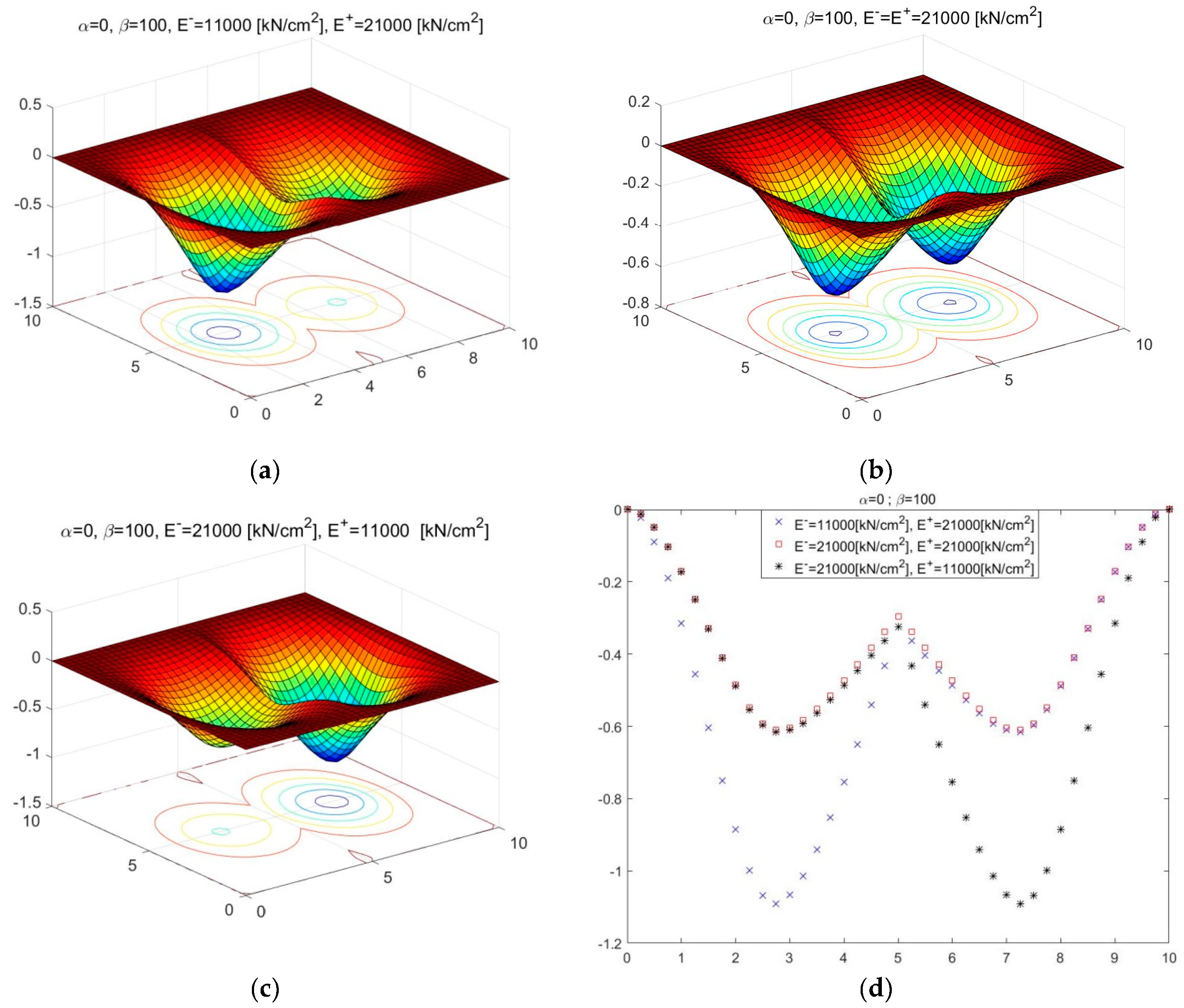
shows the results that are obtained. $\mathsf{\alpha }=0$ means that the hinge can ideally move on the common boundary of the plate system, whereas $\mathsf{\beta }=\mathrm{c}\mathrm{o}\mathrm{n}\mathrm{s}\mathrm{t}.$ indicates the presence of support with finite hardness under the hinge. In a special case, the numerical solutions that are obtained for $\mathsf{\beta }=100$ are given in Figure 2a–c. For comparison of the results, the cross sections at ${\mathrm{x}}_2={\ell }_2/2$ are shown in Figure 2d.

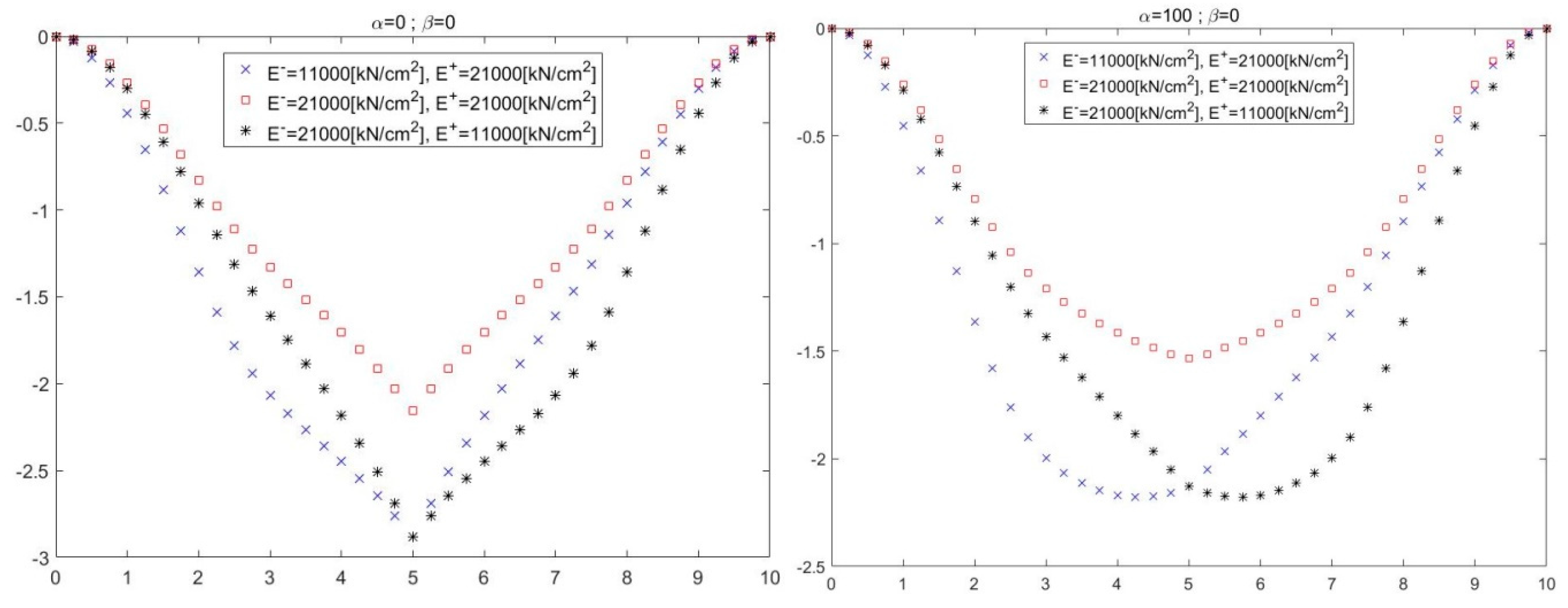
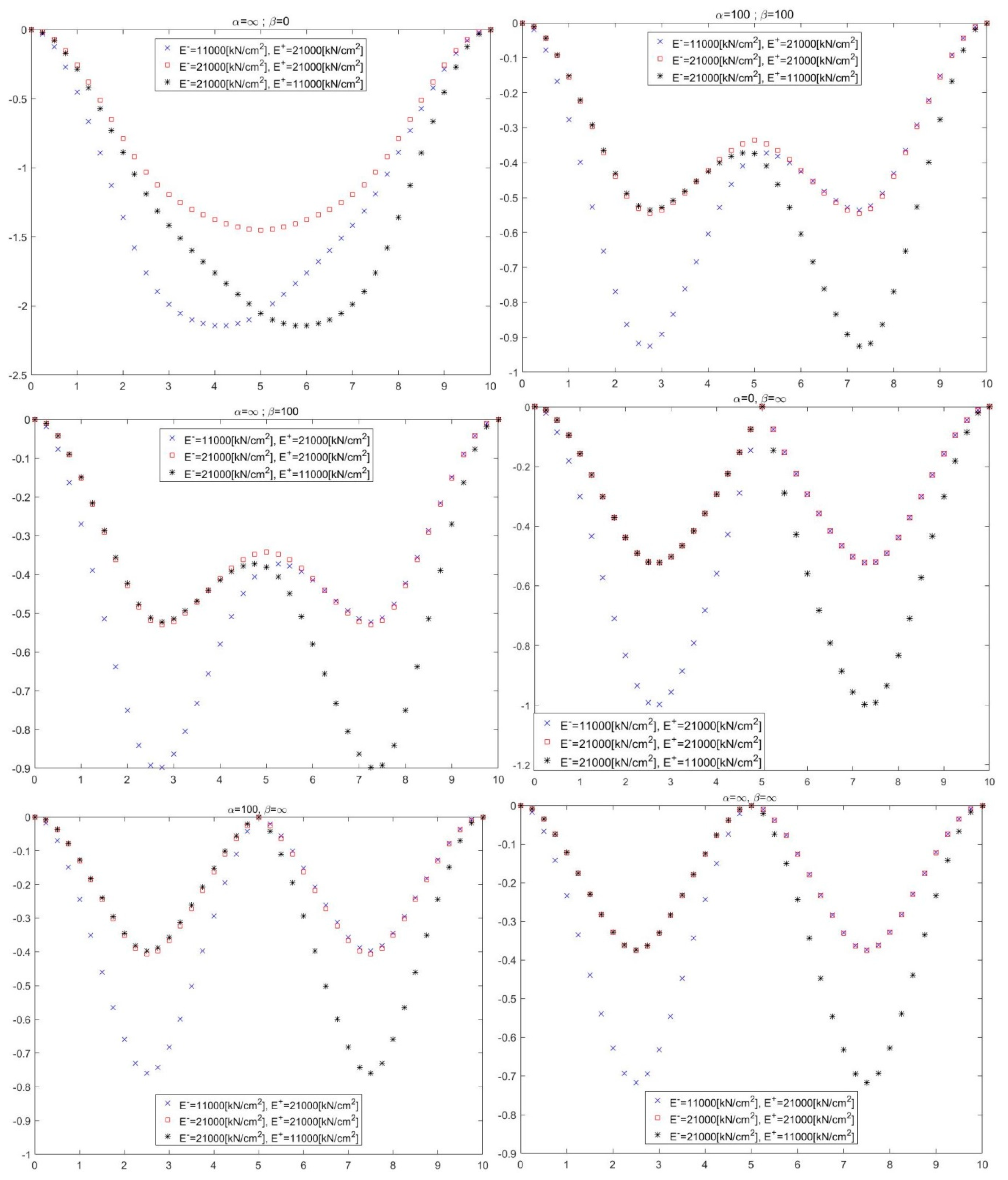
Figure 3 shows the cross sections of the numerical solutions obtained for the bending problem of the plate system at different $\mathsf{\alpha }$ and $\mathsf{\beta }$ values.

The following tables show the values of the maximal bending that corresponds to the constant force of the computer experiments given above in the geometric interpretations. The results are presented in Table 2 and

Table 3. The effect of modulus of elasticity $\mathrm{E}$ on maximal bending (cm) depending on the change of $\mathsf{\alpha }$ and $\mathsf{\beta }$ in the plate system when the simply supported condition is given on the boundaries (${\mathsf{\nu }}^{-}={\mathsf{\nu }}^{+}=0.3$ ).

		$\begin{array}{l}{\mathbf{E}}^{-}=\mathrm{11,000} [\mathbf{k}\mathbf{N}/\mathbf{c}{\mathbf{m}}^2], \\ {\mathbf{E}}^{+}=\mathrm{21,000} [\mathbf{k}\mathbf{N}/\mathbf{c}{\mathbf{m}}^2]\end{array}$			${\mathbf{E}}^{-}={\mathbf{E}}^{+}=\mathrm{21,000} [\mathbf{k}\mathbf{N}/\mathbf{c}{\mathbf{m}}^2]$			$\begin{array}{l}{\mathbf{E}}^{-}=\mathrm{21,000} [\mathbf{k}\mathbf{N}/\mathbf{c}{\mathbf{m}}^2],\\ {\mathbf{E}}^{+}=\mathrm{11,000} [\mathbf{k}\mathbf{N}/\mathbf{c}{\mathbf{m}}^2]\end{array}$
		${\mathsf{\omega }}_{\mathbf{max}}^{-}$	${\mathsf{\omega }}_{\mathbf{max}}^0$	${\mathsf{\omega }}_{\mathbf{max}}^{+}$	${\mathsf{\omega }}_{\mathbf{max}}^{-}$	${\mathsf{\omega }}_{\mathbf{max}}^0$	${\mathsf{\omega }}_{\mathbf{max}}^{+}$	${\mathsf{\omega }}_{\mathbf{max}}^{-}$	${\mathsf{\omega }}_{\mathbf{max}}^0$	${\mathsf{\omega }}_{\mathbf{max}}^{+}$
$\mathsf{\alpha }=0$	$\mathsf{\beta }=0$	8.4661	8.8137	8.3550	6.2564	6.5669	6.2564	8.3550	8.8137	8.4661
	$\mathsf{\beta }=100$	1.8143	0.3946	1.0167	1.0094	0.3643	1.0094	1.0167	0.3946	1.8143
	$\mathsf{\beta }=\infty$	1.6764	0	0.8783	0.8782	0	0.8782	0.8783	0	1.6764
$\mathsf{\alpha }=100$	$\mathsf{\beta }=0$	5.9141	5.8201	5.6692	4.1040	4.1431	4.1040	5.6692	5.8201	5.9141
	$\mathsf{\beta }=100$	1.3656	0.4571	0.7930	0.8141	0.4193	0.8141	0.7930	0.4571	1.3656
	$\mathsf{\beta }=\infty$	1.1113	0	0.5805	0.5969	0	0.5969	0.5805	0	1.1113
$\mathsf{\alpha }=\infty$	$\mathsf{\beta }=0$	5.7824	5.6090	5.4816	3.9034	3.9150	3.9034	5.4816	5.6090	5.7824
	$\mathsf{\beta }=100$	1.3040	0.4648	0.7624	0.7759	0.4287	0.7759	0.7624	0.4648	1.3040
	$\mathsf{\beta }=\infty$	1.0330	0	0.5392	0.5404	0	0.5404	0.5392	0	1.0330

for different values of $\mathsf{\alpha }$, $\mathsf{\beta }$, respectively, when the clamped boundary conditions and the simply supported boundary conditions are given for the boundaries of the system. Furthermore, the values of ${\mathsf{\omega }}_{\max }^{-} [\mathrm{c}\mathrm{m}]$, ${\mathsf{\omega }}_{\max }^0 [\mathrm{c}\mathrm{m}]$, and ${\mathsf{\omega }}_{\max }^{+} [\mathrm{c}\mathrm{m}]$ shown in the tables below are the bending values that occurred on the left plate, the common border ${\mathrm{x}}_1=0$, and the right plate, respectively.

7. Conclusions

This study obtained the transmission conditions on the common boundary in the biharmonic equation given by the discontinuous coefficient by using the functional approximation method, and analyzed the numerical results. The method that was used here may be used to find the numerical solution of problems expressed by mathematical models of differential equations with discontinuous coefficients. The same approach can be used to derive the sizes and mechanical properties of the plates forming the system.

References

1. Reddy, J.N. Theory and Analysis of Elastic Plates and Shells, 2nd ed.; CRC/Taylor & Francis: Boca Raton, FL, USA , 2007. [Google Scholar]
2. Batista, M. An exact theory of the bending of transversely inextensible elastic plates. Acta Mech. 2015, 226, 2899–2924. [Google Scholar] [CrossRef]
3. Piltner, R. The derivation of a thick and thin plate formulation without ad hoc assumptions. J. Elast. 1992, 29, 133–173. [Google Scholar] [CrossRef]
4. Wang, F.Y. 2-Dimensional theories deduced from 3-dimensional theory for a transversely isotropic body. 1. Plate problems. Int. J. Solids Struct. 1990, 26, 455–470. [Google Scholar]
5. Wang, F.Y. Two-dimensional theories deduced from three-dimensional theory for a transversely isotropic body. II: Plane problems. Int. J. Solids Struct. 1991, 28, 161–177. [Google Scholar]
6. Lim, C.W.; Cui, S.; Yao, W.A. On new symplectic elasticity approach for exact bending solutions of rectangular thin plates with two opposite sides simply supported. Int. J. Solids Struct. 2007, 44, 5396–5411. [Google Scholar] [CrossRef]
7. Lim, C.W.; Yao, W.A.; Cui, S. Benchmark symplectic solutions for bending of corner-supported rectangular thin plates. IES J. Part A: Civ. Struct. Eng. 2008, 1, 106–115. [Google Scholar] [CrossRef]
8. Shuang, C. Symplectic Elasticity Approach for Exact Bending Solutions of Rectangular Thin Plates. Master’s Thesis, City University of Hong Kong, Hong Kong, China, 2007. [Google Scholar]
9. Hasanov, A. Monotonicity of nonlinear boundary value problems related to deformation theory of plasticity. Math. Probl. Eng. 2006, 2006, 58143. [Google Scholar] [CrossRef]
10. Hasanov, A. Variational approach to non-linear boundary value problems for elasto-plastic incompressible bending plate. Int. J. Nonlinear Mech. 2007, 42, 711–721. [Google Scholar] [CrossRef]
11. Carrera, E. Theories and finite elements for multilayered, anisotropic, composite plates and shells. Arch. Comput. Methods Eng. 2002, 9, 87–140. [Google Scholar] [CrossRef]
12. Hohe, J.; Becker, W. Effective stress–strain relations for two-dimensional cellular sandwich cores: Homogenization, material models, and properties. Trans. ASME Appl. Mech. Rev. 2002, 55, 61–87. [Google Scholar] [CrossRef]
13. Kant, T.; Swaminathan, K. Estimation of transverse/interlaminar stresses in laminated composites—A selective review and survey of current developments. Compos. Struct. 2000, 49, 65–75. [Google Scholar] [CrossRef]
14. Noor, A.K.; Burton, W.S. Assessment of shear deformation theories for multilayered composite plates. Trans. ASME Appl. Mech. Rev. 1989, 42, 1–13. [Google Scholar] [CrossRef]
15. Noor, A.K.; Burton, W.S.; Bert, C.W. Computational models for sandwich panels and shells. Trans. ASME Appl. Mech. Rev. 1996, 49, 155–199. [Google Scholar] [CrossRef]
16. Grossi, R.O. Boundary value problems for anisotropic plates with internal line hinges. Acta Mech. 2012, 223, 125–144. [Google Scholar] [CrossRef]
17. Quintana, M.V.; Grossi, R.O. Free vibrations of a generally restrained rectangular plate with an internal line hinge. Appl. Acoust. 2012, 73, 356–365. [Google Scholar] [CrossRef]
18. Raffo, J.; Quintana, M.V. Natural vibrations of anisotropic plates with an internal curved line. Int. J. Mech. Sci. 2017, 120, 301–310. [Google Scholar] [CrossRef]
19. Xiang, Y.; Reddy, J.N. Natural vibration of rectangular plates with an internal line hinge using the first order shear deformation plate theory. J. Sound Vib. 2003, 263, 285–297. [Google Scholar] [CrossRef]
20. Xiang, Y.; Wang, C.M.; Wang, C.Y.; Su, G.H. Ritz buckling analysis of rectangular plates with internal hinge. J. Eng. Mech. 2003, 129, 683–688. [Google Scholar] [CrossRef]
21. Samarskii, A.; Andreev, V.B. Difference Methods for Elliptic Equations; Nauka: Moscow, Russia, 1976. [Google Scholar]
Figure 1. The plates system.
Mathematics 07 00244 g001
Figure 2. The bendings of the plate system corresponding to cases (i)–(iii) in (ac), and the cross sections of the bendings on x 2 = 2 / 2 in (d) in the case of α = 0 ,   β = 100 .
Mathematics 07 00244 g002
Figure 3. The cross sections for different values of α and β .
Mathematics 07 00244 g003aMathematics 07 00244 g003b