AHP-Group Decision Making Based on Consistency


Abstract
:1. Introduction
2. Background
2.1. Multiactor Decision Making (MADM)
2.2. Analytic Hierarchy Process
- (a)
- Modelling refers to the construction of a hierarchy of different levels that represent the relevant aspects of the problem (scenarios, actors, criteria, alternatives). The mission or goal hangs on the highest level. The subsequent levels contain the criteria, the first order subcriteria, the second order, etc. This continues to the last order subcriteria or attributes (characteristics of the reality that are susceptible to be measured for the alternatives); the alternatives hang from the lowest subcriteria level (attributes).
- (b)
- Valuation involves the incorporation of the preferences of the decision makers via pairwise comparisons of the elements that hang from the nodes of the hierarchy in relation to the common node. The judgements follow Saaty’s fundamental scale [2] and reflect the relative importance of one element with respect to another with regards to the criterion that is considered. They are expressed in reciprocal pairwise comparison matrices.
- (c)
- Prioritisation and synthesis determines the local, global and total priorities. Local priorities (priorities of the elements of the hierarchy with regards to the node from which they hang) are obtained from the pairwise comparison matrices using any of the existing prioritisation procedures. The Eigenvector (EGV) and the Row Geometric Mean (RGM) are the two most commonly employed. Global priorities (the priorities of the elements of the hierarchy with regards to the mission) are obtained through the principle of hierarchical composition, whilst Total priorities (the priorities of the alternatives with regards to the mission) are obtained by a multiadditive aggregation of the global priorities of each alternative.
- Aggregation of Individual Judgements: The individual pairwise comparison matrices A(k)k = 1,...,r, are first aggregated to obtain a new judgement matrix for the group A(G) = (). Then, the priority vector w(G/J) = () is derived from this new matrix using one of the existing prioritisation methods.
- Aggregation of Individual Priorities: The priority vectors are first obtained for each individual, w(k) = () and k = 1,...,r, using one of the existing prioritisation methods and then aggregated to obtain the priorities of the group w(G/P) = ().
- A(G) = () with
- w(G/P) = () with
2.3. Consistency and Compatibility in AHP
3. The Precise Consensus Consistency Matrix (PCCM)
4. Improving the PCCM’s Compatibility
4.1. Iterative Procedure
| Step 0: Initialisation Let and calculate for all : |
| Step 1: Selection of the judgement Let (r, s) be the entry for which |
| Step 2: Obtaining a PCCM entry Let |
| Step 3: Finalisation , then Stop Else let and go to Step 1. |
4.2. Case Study
- The order of the entrance of the judgements is the same for all the values considered for θ. This does not always have to happen.
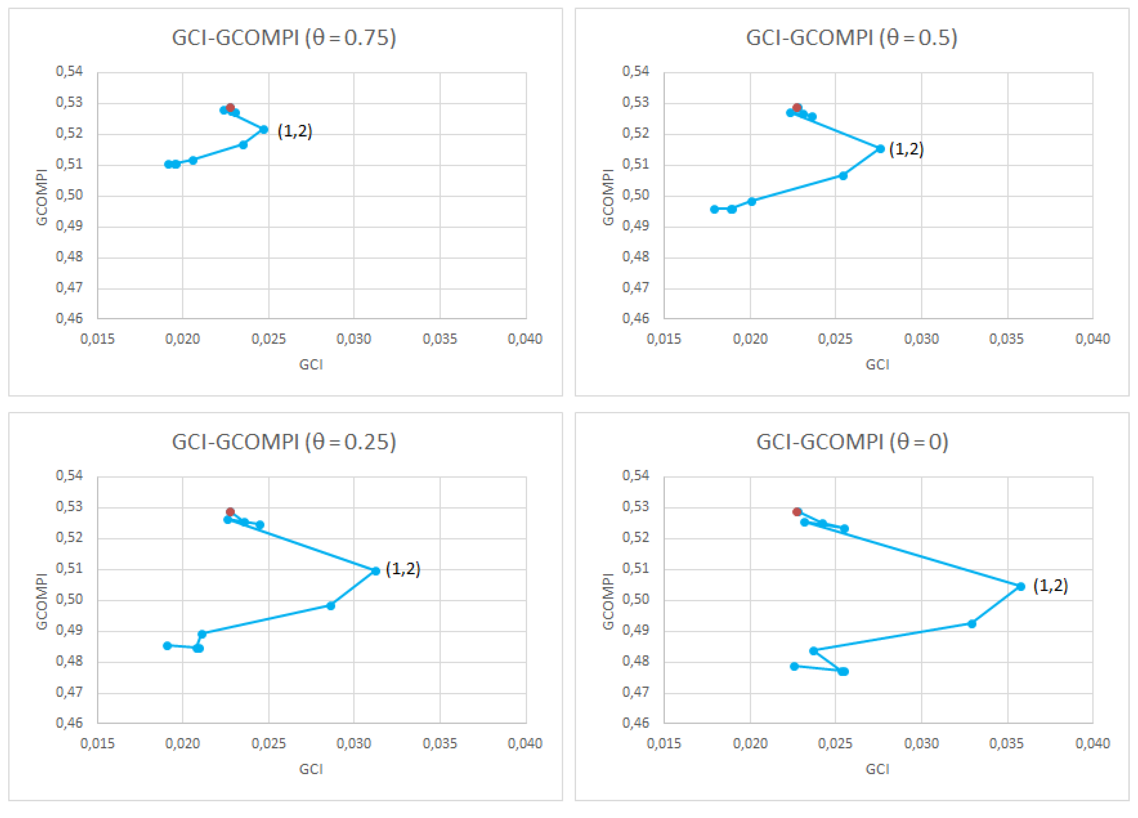
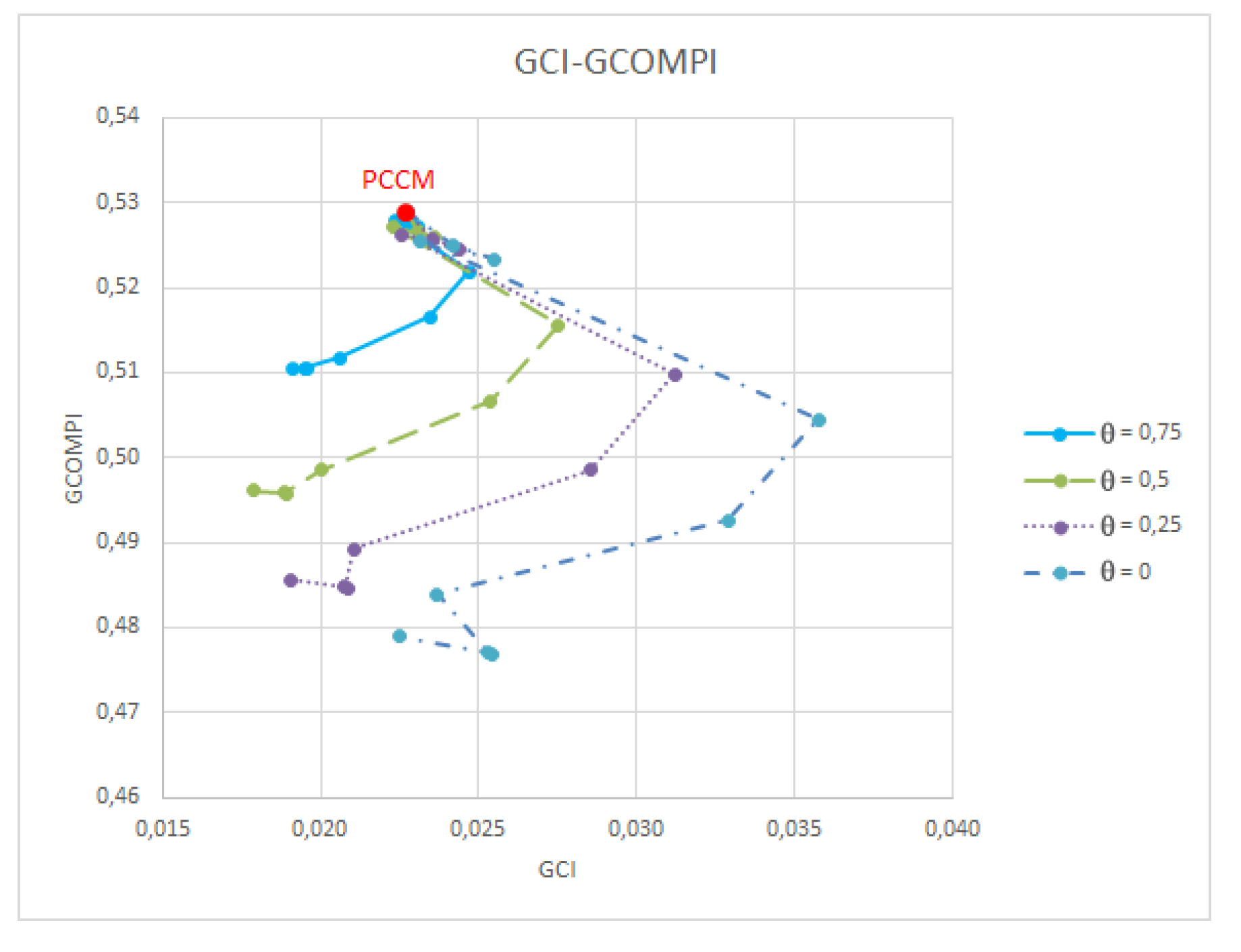
- According to the proposal followed in expression (11), the values of the compatibility indicator improve when the value of the parameter θ decreases.
- In addition to improving compatibility, the final result also improves consistency.
- The value of the compatibility indicator almost always decreases with the iterations. In just a few cases, for judgements (3,4) and (2,4), compatibility is slightly worse. The lowest value of the GCOMPI (0.477) is obtained with θ = 0 and applying the iteration procedure until the penultimate iteration. This value is only 2.8% greater than the one obtained with the AIJ.
- The consistency indicator oscillates a little until achieving the highest value at iteration t = 4 (modifying judgement (1,2)). The next iteration (modifying judgement (1,5)) is a turning point and from there the GCI reduces its value significantly (this can also be seen in Figure 1 and Figure 2). It can also be observed that the lower values of the GCI tend to be those obtained with high and intermediate values of θ. The lowest value of the GCI (0.018) is obtained with θ =0.5 and applying the iteration procedure until the last iteration. This value is 15.8% lower than that obtained with the PCCM procedure.
- The fact that in the iteration t = 8 the judgement (1,4) is not modified means that the value of the GCI is not null at the last iteration of the procedure for θ = 0.
5. Conclusions
- (i)
- For the first time, the procedure followed to solve the optimisation problem that arises in each iteration of the calculation algorithm of the PCCM has been explained in detail. The consideration of different weights for decision makers greatly increases the difficulty of the optimisation problem, and it has been necessary to study all of the possible situations that could occur.
- (ii)
- The work presents a proposal to improve the compatibility of PCCM matrices. As previously mentioned, whilst the PCCM gives much better values than other procedures with regards to consistency, its behavior in terms of compatibility is worse. Following a sequential procedure in line with their contribution to the GCOMPI, the judgments of the PCCM are modified using a combination of the initial value of the PCCM and the ratio of the priorities obtained with the AIJ procedure.
Author Contributions
Funding
Acknowledgments
Conflicts of Interest
Appendix A
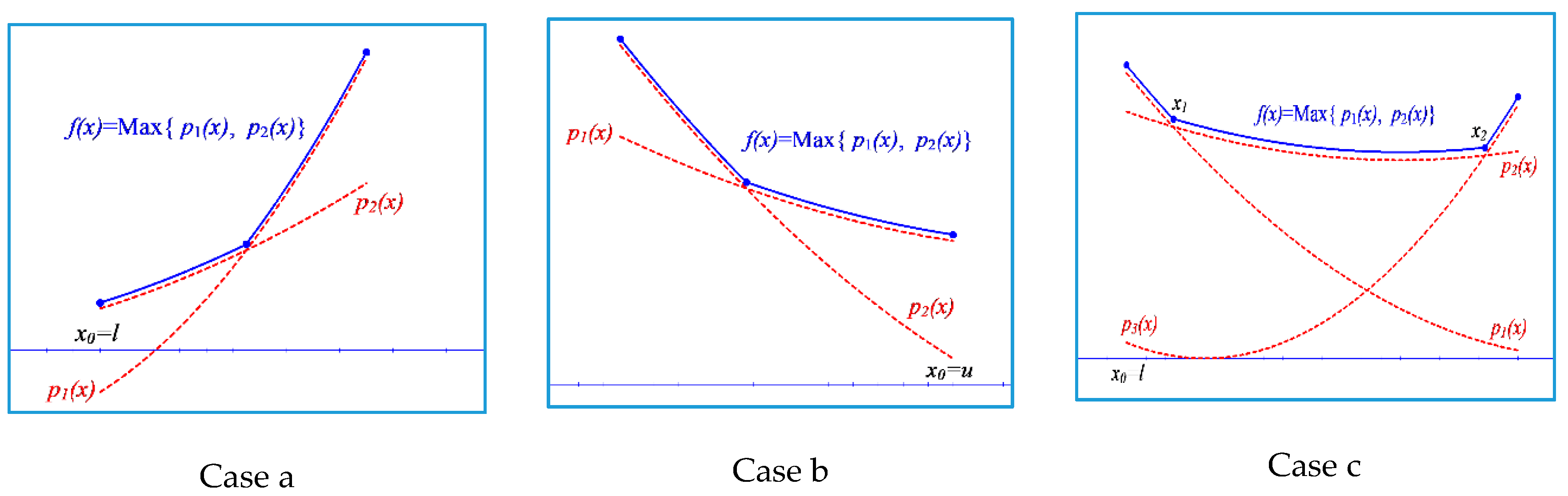
- The polynomial that is dominant in is an increasing function at this point. In this case, the solution to the optimisation problem (9) is (Figure A1a).
- The polynomial that is dominant in is a decreasing function at this point. In this case, the solution to the optimisation problem (9) is (Figure A1b).
- The polynomial that is dominant in is a decreasing function at this point. In this case, we start from this initial point and move forward until we find a section/segment in which the dominant polynomial is an increasing function (Figure A1c).
| Algorithm A1 |
| Step 1: Find and with If then . STOP If then . STOP |
| Step 2: Start from point , where the polynomial that is dominant, , is a decreasing function at this point. |
| Step 3: Calculate |
| Step 4: If the optimal solution is given by: |
| Step 5: Let be the value such that If the optimal solution is given by: Otherwise, update and and go to Step 3. |
References
- Moreno-Jiménez, J.M.; Vargas, L.G. Cognitive Multicriteria Decision Making and the Legacy of AHP. Estudios de Economía Aplicada 2018, 36, 67–80. [Google Scholar]
- Saaty, T.L. The Analytic Hierarchy Process; 2nd impression 1990, RSW Pub. Pittsburgh; Mc Graw-Hill: New York, NY, USA, 1980. [Google Scholar]
- Saaty, T.L. Group decision making and the AHP. In The Analytic Hierarchy Process; Golden, B.L., Wasil, E.A., Harker, P.T., Eds.; Springer: Berlin/Heidelberg, Germany, 1989; pp. 59–67. [Google Scholar]
- Ramanathan, R.; Ganesh, L.S. Group preference aggregation methods employed in AHP: An evaluation and intrinsic process for deriving members’ weightages. Eur. J. Oper. Res. 1994, 79, 249–265. [Google Scholar] [CrossRef]
- Forman, E.; Peniwati, K. Aggregating individual judgements and priorities with the analytic hierarchy process. Eur. J. Oper. Res. 1998, 108, 165–169. [Google Scholar] [CrossRef]
- Escobar, M.T.; Moreno-Jiménez, J.M. Aggregation of Individual Preference Structures. Group Decis. Negotiat. 2007, 16, 287–301. [Google Scholar] [CrossRef]
- Altuzarra, A.; Moreno-Jiménez, J.M.; Salvador, M. A Bayesian priorization procedure for AHP-group decision making. Eur. J. Oper. Res. 2007, 182, 367–382. [Google Scholar] [CrossRef]
- Moreno-Jiménez, J.M.; Aguarón, J.; Escobar, M.T. Decisional Tools for Consensus Building in AHP-Group Decision Making. In Proceedings of the 12th Mini Euro Conference, Brussels, Belgium, 2–5 April 2002. [Google Scholar]
- Moreno-Jiménez, J.M.; Aguarón, J.; Raluy, A.; Turón, A. A spreadsheet module for consistent AHP-consensus building. Group Decis. Negotiat. 2005, 14, 89–108. [Google Scholar]
- Moreno-Jiménez, J.M.; Aguarón, J.; Escobar, M.T. The core of consistency in AHP-group decision making. Group Decis. Negotiat. 2008, 17, 249–265. [Google Scholar]
- Escobar, M.T.; Aguarón, J.; Moreno-Jiménez, J.M. Some extensions of the Precise Consistency Consensus Matrix. Decis. Support Syst. 2015, 74, 67–77. [Google Scholar] [CrossRef]
- Aguarón, J.; Escobar, M.T.; Moreno-Jiménez, J.M. The precise consistency consensus matrix in a local AHP-group decision making context. Ann. Oper. Res. 2016, 245, 245–259. [Google Scholar] [CrossRef]
- Moreno-Jiménez, J.M. Los Métodos Estadísticos en el Nuevo Método Científico. In Información Económica y Técnicas de Análisis en el Siglo XXI; Casas, J.M., Pulido, A., Eds.; INE: Madrid, Spain, 2003; pp. 331–348. [Google Scholar]
- De Bono, E. Lateral Thinking: Creativity Step by Step; Harper & Row: New York, NY, USA, 1970. [Google Scholar]
- Salvador, M.; Altuzarra, A.; Gargallo, M.P.; Moreno-Jiménez, J.M. A Bayesian Approach for maximising inner compatibility in AHP-Systemic Decision Making. Group Decis. Negotiat. 2015, 24, 655–673. [Google Scholar] [CrossRef]
- Moreno-Jiménez, J.M.; Gargallo, M.P.; Salvador, M.; Altuzarra, A. Systemic Decision Making: A Bayesian Approach in AHP. Ann. Oper. Res. 2016, 245, 261–284. [Google Scholar] [CrossRef]
- Barzilai, J.; Golany, B. AHP rank reversal, normalization and aggregation rules. INFOR 1994, 32, 57–63. [Google Scholar] [CrossRef]
- Escobar, M.T.; Aguarón, J.; Moreno-Jiménez, J.M. A Note on AHP Group Consistency for the Row Geometric Mean Priorization Procedure. Eur. J. Oper. Res. 2004, 153, 318–322. [Google Scholar] [CrossRef]
- Aguarón, J.; Moreno-Jiménez, J.M. The geometric consistency index: Approximate thresholds. Eur. J. Oper. Res. 2003, 147, 137–145. [Google Scholar] [CrossRef]
- Aguarón, J.; Escobar, M.T.; Moreno-Jiménez, J.M. Consistency stability intervals for a judgement in AHP decision support systems. Eur. J. Oper. Res. 2003, 145, 382–393. [Google Scholar] [CrossRef]
- Moreno-Jiménez, J.M. An AHP/ANP Multicriteria Methodology to Estimate the Value and Transfers Fees of Professional Football Players. In Proceedings of the ISAHP 2011, Sorrento, Italy, 14–18 June 2011. [Google Scholar]
- Golany, B.; Kress, M. A multicriteria evaluation of methods for obtaining weights from ratio-scale matrices. Eur. J. Oper. Res. 1993, 69, 210–220. [Google Scholar] [CrossRef]
- Dong, Y.; Zhang, G.; Hong, W.C.; Xu, Y. Consensus models for AHP group decision making under row geometric mean prioritization method. Decis. Support Syst. 2010, 49, 281–289. [Google Scholar] [CrossRef]
- Moreno-Jiménez, J.M.; Gómez-Bahillo, C.; Sanaú, J. Viabilidad Integral de Proyectos de Inversión Pública. Valoración económica de los aspectos sociales. In Anales de Economía Aplicada XXIII; Pires, J.R., Monteiro, J.D., Eds.; Delta: Madrid, Spain, 2009; pp. 2551–2562. [Google Scholar]
- Turón, A.; Aguarón, J.; Escobar, M.T.; Moreno-Jiménez, J.M. A Decision Support System and Visualisation Tools for AHP-GDM. Int. J. Decis. Supports Syst. Technol. 2019, 11, 1–19. [Google Scholar] [CrossRef]

| DM1 | A1 | A2 | A3 | A4 | A5 | DM2 | A1 | A2 | A3 | A4 | A5 | DM3 | A1 | A2 | A3 | A4 | A5 |
|---|---|---|---|---|---|---|---|---|---|---|---|---|---|---|---|---|---|
| A1 | 1 | 3 | 5 | 8 | 6 | A1 | 1 | 3 | 7 | 9 | 5 | A1 | 1 | 5 | 7 | 7 | 5 |
| A2 | - | 1 | 3 | 5 | 4 | A2 | - | 1 | 3 | 7 | 1 | A2 | - | 1 | 1 | 5 | 1 |
| A3 | - | - | 1 | 3 | 2 | A3 | - | - | 1 | 5 | 1/5 | A3 | - | - | 1 | 5 | 1/3 |
| A4 | - | - | - | 1 | 1/3 | A4 | - | - | - | 1 | 1/5 | A4 | - | - | - | 1 | 1/5 |
| A5 | - | - | - | - | 1 | A5 | - | - | - | - | 1 | A5 | - | - | - | - | 1 |
| Priorities | DM1 | DM2 | DM3 |
|---|---|---|---|
| A1 | 0.513 | 0.520 | 0.560 |
| A2 | 0.251 | 0.195 | 0.135 |
| A3 | 0.115 | 0.072 | 0.101 |
| A4 | 0.042 | 0.030 | 0.035 |
| A5 | 0.079 | 0.182 | 0.168 |
| Rankings | 1-2-3-5-4 | 1-2-5-3-4 | 1-5-2-3-4 |
| GCIs | 0.143 | 0.303 | 0.298 |
| PCCM | A1 | A2 | A3 | A4 | A5 |
|---|---|---|---|---|---|
| A1 | 1 | 2.05 | 5.51 | 9 | 3.17 |
| A2 | 0.49 | 1 | 3 | 6.08 | 1.74 |
| A3 | 0.18 | 0.33 | 1 | 2.71 | 0.68 |
| A4 | 0.11 | 0.16 | 0.37 | 1 | 0.35 |
| A5 | 0.32 | 0.58 | 1.47 | 2.4 | 1 |
| Priorities | PCCM | AIJ | Dong |
|---|---|---|---|
| A1 | 0.467 | 0.533 | 0.531 |
| A2 | 0.255 | 0.208 | 0.216 |
| A3 | 0.095 | 0.096 | 0.099 |
| A4 | 0.044 | 0.037 | 0.038 |
| A5 | 0.139 | 0.125 | 0.116 |
| Rankings | 1-2-5-3-4 | 1-2-5-3-4 | 1-2-5-3-4 |
| PCCM | AIJ | Dong | |
|---|---|---|---|
| GCI | 0.023 | 0.122 | 0.069 |
| CVN | 0 | 0.018 | 0.018 |
| GCOMPI | 0.529 | 0.464 | 0.472 |
| PVN | 0.136 | 0.136 | 0.136 |
| Iteration° | t = 0 | t = 1 | t = 2 | t = 3 | t = 4 | t = 5 | t = 6 | t = 7 | t = 8 | t = 9 | t = 10 |
|---|---|---|---|---|---|---|---|---|---|---|---|
| Modif. Judg. | - | (3,5) | (2,5) | (3,4) | (1,2) | (1,5) | (2,3) | (4,5) | (1,4) | (1,3) | (2,4) |
| GCI | 0.023 | 0.023 | 0.023 | 0.022 | 0.025 | 0.023 | 0.021 | 0.019 | ° | 0.020 | 0.019 |
| GCOMPI | 0.529 | 0.528 | 0.527 | 0.528 | 0.522 | 0.517 | 0.512 | 0.511 | ° | 0.511 | 0.511 |
| Iteration° | t = 0 | t = 1 | t = 2 | t = 3 | t = 4 | t = 5 | t = 6 | t = 7 | t = 8 | t = 9 | t = 10 |
|---|---|---|---|---|---|---|---|---|---|---|---|
| Modif. Judg. | - | (3,5) | (2,5) | (3,4) | (1,2) | (1,5) | (2,3) | (4,5) | (1,4) | (1,3) | (2,4) |
| GCI | 0.023 | 0.023 | 0.024 | 0.022 | 0.028 | 0.025 | 0.020 | 0.019 | ° | 0.019 | 0.018 |
| GCOMPI | 0.529 | 0.527 | 0.526 | 0.527 | 0.516 | 0.507 | 0.499 | 0.496 | ° | 0.496 | 0.496 |
| Iteration° | t = 0 | t = 1 | t = 2 | t = 3 | t = 4 | t = 5 | t = 6 | t = 7 | t = 8 | t = 9 | t = 10 |
|---|---|---|---|---|---|---|---|---|---|---|---|
| Modif. Judg. | - | (3,5) | (2,5) | (3,4) | (1,2) | (1,5) | (2,3) | (4,5) | (1,4) | (1,3) | (2,4) |
| GCI | 0.023 | 0.024 | 0.024 | 0.023 | 0.031 | 0.029 | 0.021 | 0.021 | ° | 0.021 | 0.019 |
| GCOMPI | 0.529 | 0.526 | 0.525 | 0.526 | 0.510 | 0.499 | 0.489 | 0.485 | ° | 0.485 | 0.486 |
| Iteration° | t = 0 | t = 1 | t = 2 | t = 3 | t = 4 | t = 5 | t = 6 | t = 7 | t = 8 | t = 9 | t = 10 |
|---|---|---|---|---|---|---|---|---|---|---|---|
| Modif. Judg. | - | (3,5) | (2,5) | (3,4) | (1,2) | (1,5) | (2,3) | (4,5) | (1,4) | (1,3) | (2,4) |
| GCI | 0.023 | 0.024 | 0.025 | 0.023 | 0.036 | 0.033 | 0.024 | 0.025 | ° | 0.025 | 0.023 |
| GCOMPI | 0.529 | 0.525 | 0.523 | 0.525 | 0.505 | 0.493 | 0.484 | 0.477 | ° | 0.477 | 0.479 |
| Modified PCCM (θ = 0.75) | A1 | A2 | A3 | A4 | A5 | Modified PCCM (θ = 0.5) | A1 | A2 | A3 | A4 | A5 |
| A1 | 1 | 2.17 | 5.52 | 9 | 3.41 | A1 | 1 | 2.29 | 5.52 | 9 | 3.67 |
| A2 | 0.46 | 1 | 2.76 | 5.97 | 1.72 | A2 | 0.44 | 1 | 2.55 | 5.86 | 1.70 |
| A3 | 0.18 | 0.36 | 1 | 2.68 | 0.70 | A3 | 0.18 | 0.39 | 1 | 2.66 | 0.72 |
| A4 | 0.11 | 0.17 | 0.37 | 1 | 0.34 | A4 | 0.11 | 0.17 | 0.38 | 1 | 0.32 |
| A5 | 0.29 | 0.58 | 1.42 | 2.97 | 1 | A5 | 0.27 | 0.59 | 1.38 | 3.11 | 1 |
| Modified PCCM (θ = 0.25) | A1 | A2 | A3 | A4 | A5 | Modified PCCM (θ = 0) | A1 | A2 | A3 | A4 | A5 |
| A1 | 1 | 2.42 | 5.53 | 9 | 3.96 | A1 | 1 | 2.56 | 5.54 | 9 | 4.26 |
| A2 | 0.41 | 1 | 2.35 | 5.75 | 1.68 | A2 | 0.39 | 1 | 2.16 | 5.64 | 1.66 |
| A3 | 0.18 | 0.43 | 1 | 2.64 | 0.75 | A3 | 0.18 | 0.46 | 1 | 2.61 | 0.77 |
| A4 | 0.11 | 0.17 | 0.38 | 1 | 0.31 | A4 | 0.11 | 0.18 | 0.38 | 1 | 0.29 |
| A5 | 0.25 | 0.59 | 1.34 | 3.25 | 1 | A5 | 0.23 | 0.60 | 1.30 | 3.39 | 1 |
| Priorities | PCCM (θ = 1) | θ = 0.75 | θ = 0.5 | θ = 0.25 | θ = 0 |
|---|---|---|---|---|---|
| A1 | 0.467 | 0.477 | 0.488 | 0.498 | 0.508 |
| A2 | 0.255 | 0.245 | 0.236 | 0.227 | 0.218 |
| A3 | 0.095 | 0.096 | 0.098 | 0.099 | 0.101 |
| A4 | 0.044 | 0.044 | 0.043 | 0.043 | 0.042 |
| A5 | 0.139 | 0.137 | 0.135 | 0.133 | 0.131 |
| Rankings | 1-2-5-3-4 | 1-2-5-3-4 | 1-2-5-3-4 | 1-2-5-3-4 | 1-2-5-3-4 |
© 2019 by the authors. Licensee MDPI, Basel, Switzerland. This article is an open access article distributed under the terms and conditions of the Creative Commons Attribution (CC BY) license (http://creativecommons.org/licenses/by/4.0/).
Share and Cite
Aguarón, J.; Escobar, M.T.; Moreno-Jiménez, J.M.; Turón, A. AHP-Group Decision Making Based on Consistency. Mathematics 2019, 7, 242. https://doi.org/10.3390/math7030242
Aguarón J, Escobar MT, Moreno-Jiménez JM, Turón A. AHP-Group Decision Making Based on Consistency. Mathematics. 2019; 7(3):242. https://doi.org/10.3390/math7030242
Chicago/Turabian StyleAguarón, Juan, María Teresa Escobar, José María Moreno-Jiménez, and Alberto Turón. 2019. "AHP-Group Decision Making Based on Consistency" Mathematics 7, no. 3: 242. https://doi.org/10.3390/math7030242
APA StyleAguarón, J., Escobar, M. T., Moreno-Jiménez, J. M., & Turón, A. (2019). AHP-Group Decision Making Based on Consistency. Mathematics, 7(3), 242. https://doi.org/10.3390/math7030242