First-Arrival Travel Times Picking through Sliding Windows and Fuzzy C-Means

Abstract

First-arrival picking is a critical step in seismic data processing. This paper proposes the first-arrival picking through sliding windows and fuzzy c-means (FPSF) algorithm with two stages. The first stage detects a range using sliding windows on vertical and horizontal directions. The second stage obtains the first-arrival travel times from the range using fuzzy c-means coupled with particle swarm optimization. Results on both noisy and preprocessed field data show that the FPSF algorithm is more accurate than classical methods.

1. Introduction

Seismic refraction data analysis is one of the principal methods for near-surface modeling [1,2,3,4]. A critical step of the method is first-arrival picking for direct and head waves. It influences the effectiveness of many steps such as static correction [5,6] and velocity modeling [7]. Misidentifications of these arrival times may have significant effects on the hypocenters [8]. However, the raw seismic traces are always contaminated by strong background noise with complex near-surface conditions [7]. The main challenge is to accurately extract the first arrivals under the noise interference [9,10] and irregular topography [11]. According to Akram and Eaton [8], there is an urgent need for automatic picking methods as the scale of seismic data continues to grow.

There are three main types of first-arrival picking methods. The first is Coppens’ method [12] and its variants. It uses energy ratios within two amplitude windows to process the data [12]. Al-Ghamdi and Saeed [13] improved this method by using adaptive thresholds. The multi-window algorithm [14] uses three moving windows instead. Moreover, it distinguishes signals from noise using the average of the absolute amplitudes in each window. Sabbione and Velis [15] used a modified form of Coppens’ method along with entropy and fractal-dimension methods to pick first-arrival travel times. The second is the direct correlation method [16]. The direct correlation method was proposed by Molyneux and Schmitt [16]. It uses the maximum cross correlation value as a criterion [16], which fails in data sets with low signal-to-noise ratio (S/N). The third is the backpropagation neural networks method [17]. It applies backpropagation neural networks in first-arrival refraction event picking and seismic data trace editing [17].

Recently, a new algorithm based on fuzzy c-means is proposed to deal with low signal-to-noise ratio data [18]. It divides microseismic data into two clusters according to the different levels of similarity between the signals and noise. Thus, the initial time of the signal cluster is regarded as the first-arrival time. Others have reported many automatic picking schemes such as digital image segmentation [19], STA/LTA method [20,21], Akaike information criterion [22], fractal-based algorithm [23] and TDEE [11]. However, the detection accuracy of existing algorithms is still unsatisfactory.

In this paper, we propose the first-arrival picking through sliding windows and fuzzy c-means (FPSF) algorithm. Figure 1 illustrates the overall structure of our algorithm through an example. In the range detection stage, each trace is processed with a vertical sliding window to seek the first-arrival interval of each trace. Then, the horizontal window is employed to adjust the window for each trace. In this way, the first-arrival range is identified. In the first-arrival travel times picking stage, a particle swarm optimization (PSO) algorithm seeks original cluster centers. Finally, a fuzzy c-means (FCM) picks the first-arrival travel times.

FPSF presents two new features to handle the challenge mentioned earlier. One is to introduce a range detection stage before first-arrival picking. We design a range detection technique using sliding windows on vertical and horizontal directions. On the one hand, the energy of single trace will abruptly shift in the first-arrival interval. Hence, a vertical sliding window is employed for keeping track of inner-trace change. The quality of the window is measured by the difference between its upper and lower parts, and its position in the trace. It finds the interval where the energy values suddenly shift the most. On the other hand, the first-arrival travel times of adjacent traces are approximate. Hence, a horizontal sliding window is employed for keeping track of inter-trace change. It adjusts the locations of vertical windows to ensure their similarities. All vertical windows of each trace consist of first-arrival range. With this technique, the data size is decreased dramatically, and the accuracy can be improved.

The other is to employ PSO and FCM for clustering seismic data. FCM is successful in image processing, so the application to our data is expected [18]. The data is restricted to the first-arrival range. First, an improved particle swarm optimization is used to determine original cluster centers. Second, an improved fuzzy c-means which has original cluster centers will pick up first-arrival travel times among the range.

Experiments are undertaken on two field data sets. We compare FPSF with some methods including modified Coppens’ method (MCM) [15], the direct correlation method (DC) [16], and backpropagation neural networks method (BNN) [17]. Results show that FPSF is accurate. FPSF can be used in many domains such as image processing and seismic data processing.

The rest of the paper is organized as follows. In Section 2, we review some related works. In Section 3, we build a data model, define the first-arrival picking problem and introduce some concepts. In Section 4, we elaborate on the principle of the new method of this paper. In the sequel, two field data sets are experimented to verify the effectiveness of the method in Section 5. Finally, Section 6 summarizes this paper.

2. Related Works

The history of seismic refraction data analysis can be traced back to the 1920s [6]. Seismic refraction data analysis tasks include deconvolution [24], dynamic correction [25], static correction [26,27], speed analysis [28], and migration [29]. Picking first arrivals [19] is an important pre-processing stage for these tasks. For example, the effectiveness of static corrections depends on the precise of the first arrivals [6,15].

There are three strategies in the development of picking first arrivals. The manual strategy relies solely on the experts, therefore it is time-consuming and occasionally inaccurate [15,19,23,30]. To make the matter worse, this strategy can lead to biased and inconsistent picks because it relies on the subjectivity of the selection operator [15].

The man–machine interaction strategy provides experts with software for visual inspection [19,23,30]. The expert should identify a few first arrivals, and then the software will pick the others. In case of some difficult situations, the expert interfere with the process. Naturally, this strategy is more efficient. However, the whole procedure is still very time consuming and subjective.

The automatic strategy [15,16,23] aims to provide more efficient and intelligent solution. It requires the development of advanced machine learning and data mining algorithms. Note that this strategy does not prevent experts from intervening. Experts should check the result and correct it if necessary. Naturally, if the algorithm works well, manual intervention is rare.

Currently, there are many well-known seismic data processing systems, such as Promax [31], CGG (refering to wikipedia), Focus and Grisys [32]. They all contain the key step of picking first arrivals. Affected by data quality and parameter setting, the results of each software program are very different. Therefore, an accurate, efficient and stable algorithm for this problem is needed.

3. Preliminaries

In this section, we build a data model, define the first-arrival picking problem and introduce some basic concepts.

Table 1. Notations.

Notation	Meaning
S	The single shot gather
F	The first-arrival times
l	The vertical window size
b	The horizontal window size
$\lambda$	The starting index of the current window
a	The energy ratio weight
k	The search step size
$\mathsf{\Lambda }$	The starting index array of result windows
n	The number of traces
m	The number of samples for each trace
R	The first-arrival range matrix
$\theta$	The parameters of fitness function
$\pi$	The parameters of fitness function
B	The boundary matrix
$B_1$	The position boundary matrix
$B_2$	The velocity range matrix
g	The dimension of the input problem
f	The fitness function
M	The number of particles
${\delta }_1$	The inertia weight of each particle’s velocity
${\delta }_2$	The global influence weight
w	The inertia weight
T	The maximum iteration times
$\epsilon$	The convergent error
$x^{*}$	The solution of the best particle
U	The first-arrival range matrix
e	The number of clustering centers
$\gamma$	The fuzzy indicator
$J_{FCM}$	The objective function
$c_k$	The center of the k-th cluster
$d_k(i,j)$	The distance between $s_{i,j}$ and $c_k$

lists notations used throughout the paper.

3.1. Data Model

Single shot gather is a basic concept in the field of geophysical prospecting.

Definition 1.

A single shot gather is an $m\times n$ matrix $S=[s_{i,j}]$, where n is the number of traces, m is the number of samples for each trace, and $s_{i,j}$ is the energy value of the ith sample of the jth trace.

Figure 2a illustrates an original single shot gather with 1000 samples and 800 traces. The horizontal coordinate is the number of traces. The vertical coordinate is the number of samples. The amplitude values of samples are the energy values. Black and white points correspond to positive and negative amplitudes, respectively. To cope with different geophones and different traces, we pre-process our data normalized to the range $[-1,1]$.

3.2. First-Arrival Picking

We consider the following problem.

Problem 1.

The first-arrival picking problem.

Input: A single shot gather S;

Output: $F=[f(1),f(2),\dots ,f(n)]$, where $\forall j\in [1‥n]$, $f\left(j\right)\in [1‥m]$ is the first-arrival time of the j-th trace.

That is, for any trace j, there is exactly one sample $f(j)$ corresponding to the first-arrival travel time.

Figure 2b shows the output of first-arrival picking with the input shown in Figure 2a. Every trace has one first-arrival travel time. The red point is the first-arrival location of every trace.

3.3. Fuzzy c-Means

FCM algorithm was proposed by Dunn [33]. It was promoted as the general FCM clustering algorithm by Bezdek [34]. FCM has been used in many fields such as image segmentation [35,36,37]. The fuzzy set was conceived as a result of an attempt to come to grips with the problem of imprecisely defined categories [34]. K-means determines whether or not a group of objects form a cluster. Different from k-means, FCM determines the belonging of an object to a class with a matter of degree [34,38]. When objects X consists of k compact well separated clusters, k-means generates a limiting partition with membership functions which closely approximate the characteristic functions of the clusters. However, when X is not the union of k compact well separated clusters, the limiting partition is truly fuzzy in the sense that the values of its component membership functions differ substantially from 0 or 1 over certain regions of X. The fuzzy algorithm seems significantly less prone to the “cluster-splitting” tendency and may also be less easily diverted to uninteresting locally optimal partitions Dunn [33].

Let $O=\{o_1,o_2,\dots ,o_N\}$ be a set of objects. The standard fuzzy c-means objective function for partitioning O into e clusters is given by [37,39]:

$$min{J}_{\alpha }=\sum _{i=1}^e\sum _{k=1}^N{u}_{ik}^{\alpha }{d}_{ik}^{\beta },$$

(1)

where $u_{ik}\in [0,1]$ is the degree of $o_k$ belonging to the i-th cluster, $\alpha$ is the fuzzy indicator, $d_{ik}=\parallel o_k-c_i\parallel$ is the distance between $o_k$ and $c_i$, and $c_i$ is the center of the i-th cluster.

We also require the sum of the degrees of each object be 1, i.e., ${\sum }_{i=1}^e{u}_{ik}=1$ $\forall k\in [1‥N]$. In many applications, the Euclidean distance is employed to compute $d_{ik}$, and $\beta =2$.

3.4. Particle Swarm Optimization

Particle swarm optimization was first proposed by [40]. It is a nature-inspired meta-heuristic approach applied to solve optimisation problems in different fields [41,42,43,44,45].

For an optimisation problem with M particles. Let $x_i^{\prime }\left(t\right)$ denote the best solution that particle i has obtained until iteration t. Let $x^{*}(t)$ denote the best solution obtained among all the particles so far. To search for the optimal solution, each particle updates its velocity $v_i\left(t\right)$ and position $x_i\left(t\right)$ according to Equation (2) and (3) [46]:

$$v_i(t+1)=w{v}_j(t)+{\delta }_{1}ran{d}_1\times (x_i^{\prime }\left(t\right)-x_i\left(t\right))+{\delta }_{2}ran{d}_2\times (x^{*}\left(t\right)-x_i\left(t\right)),$$

(2)

$$x_i(t+1)=x_i\left(t\right)+v_i\left(t\right),$$

(3)

where t is the current iteration, $ran{d}_1$ and $ran{d}_2$ are the random variables in the range of $[0,1]$, ${\delta }_1$ and ${\delta }_2$ are the two positive acceleration constants to adjust relative velocity with respect to best global and local positions and the inertia weight w is used to balance the capabilities of the global exploration.

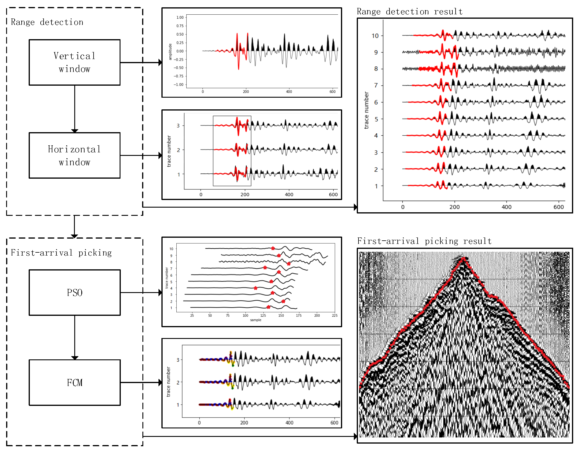
4. The Proposed Algorithm

The algorithm framework has been illustrated in Figure 1. The range detection stage is composed of vertical window sliding and horizontal window sliding. The first-arrival picking stage is composed of PSO and FCM. This section describes each stage in detail.

4.1. Range Detection

This subsection explains the range detection stage with a vertical sliding window and a horizontal sliding window.

We apply a vertical sliding window to capture the energy which is large, early and shift abrupt in each trace. Let the window size be l and the starting index of the current window of the j-th trace be ${\lambda }_j$. We design the following optimization objective function:

$$minr(l,{\lambda }_j)=a\times \frac{(1+{\sum }_{i=1}^{l/2}{s}_{i+{\lambda }_j,j})}{(1+{\sum }_{i=l/2+1}^l{s}_{i+{\lambda }_j,j})}+(1-a)\times l{\lambda }_j,$$

(4)

where a is the energy ratio weight. Here, the first part expresses the ratio between the upper and lower part of the window. The smaller the value, the larger the shift. The second part expresses the evaluation of the position of the window. The smaller the value, the earlier the travel time. The weight a is used to obtain a trade-off between these two values.

Algorithm 1 lists the vertical window sliding process. Line 1 initializes the minimal value of the object function value $r^{*}$. Lines 2 to 10 show the process of sliding a vertical window with a step size of k. Line 3 calculates the sum of the upper part of the window $us$. Line 4 calculates the sum of the lower part of the window $ls$. Line 5 computes object function value of the current window according to Equation (4). Lines 6 to 9 determine if the update condition has been reached. If so, update the minimal value of the object function value $r^{*}$ and the starting index of the vertical window ${\lambda }_j$ in Lines 7 and 8.

Algorithm 1: Vertical Window Sliding for One Trace
Input: The j-th trace $s_{·,j}=[s_{1,j},s_{2,j},\dots ,s_{m,j}]$, window size l, ratio weight a and search step size k.
Output: The starting index of the result window ${\lambda }_j$.
Method: verticalSliding.
1:	$r^{*}=+\infty$; // Initialize
2:	for ($i=1$ step k to $m-l$) do
3:	$us={\sum }_i^{i+\frac{l}{2}-1}{s}_{i,j}$; // The sum of the upper part
4:	$ls={\sum }_{i+\frac{l}{2}}^{i+l}{s}_{i,j}$; // The sum of the lower part
5:	$r=a\times (1+us)/(1+ls)+(1-a)\times l\times i$; // Compute r
6:	if ($r<r^{*}$) then
7:	$r^{*}=r$;
8:	${\lambda }_j=i$; // Update the starting index
9:	end if
10:	end for
11:	return${\lambda }_j$;

We apply a horizontal window to adjust the neighboring first-arrival intervals determined by the vertical windows. Median filtering is employed to smooth the first-arrival intervals in the window to ensure their similarity.

Definition 2.

First-arrival range matrix is an $l\times n$ matrix $R=[s_{i,j}]$, where l is the size of vertical window and n is the number of traces. It saves the first-arrival range including first arrivals. This matrix stores the range of the first arrivals. The size of the original data set S has been reduced from $m\times n$ to $l\times n$.

Algorithm 2 lists the horizontal window sliding process. Lines 1 to 9 show the process of sliding a horizontal window. Line 2 moves the horizontal window in step size b. Line 3 obtains the median of the window m. Lines 4 to 7 determine whether the difference between each element in the window and the median is too large. If so, update this value with a large difference to the median in Line 6.

After the above steps, range detection stage has been completed and the first-arrival range expressed by the first-arrival range matrix (R) has been confirmed. This is one kind of dimensionality reduction techniques [47] and data size is directly reduced by 90%. Just as pre-processing can help increase the accuracy [48], range detection stage can be viewed as a pre-processing stage.

Algorithm 2: Horizontal Window Sliding
Input: The starting index array of result windows $\mathsf{\Lambda }=[{\lambda }_1,{\lambda }_2,\dots ,{\lambda }_n]$, vertical window size l and horizontal window size b.
Output: Range starting index array $\mathsf{\Lambda }$.
Method: horizontalSliding.
1:	for ($i=1$ to $\frac{n}{b}$) do
2:	$H=[{\lambda }_{(i-1)\times b+1},{\lambda }_{(i-1)\times b+2},\dots ,{\lambda }_{i\times b}]$; // Move the horizontal window
3:	$m=median(H)$; // Get the median of the window
4:	for ($j=1$ to b) do
5:	if ($abs(H[j]-m)⩾\frac{l}{2}$) then
6:	$\mathsf{\Lambda }[j+(i-1)\times b]=m$; // Update the value with a large difference
7:	end if
8:	end for
9:	end for
10:	return$\mathsf{\Lambda }$;

4.2. First-Arrival Picking from the Range

This subsection explains the first-arrival picking stage with PSO and FCM. The data field at this stage is the first-arrival range confirmed by range detection stage.

We employ PSO to find the original clustering centers of FCM according to the advantages of PSO including global optimization and fast convergence [49]. Specifically, we use the following fitness function:

$$f(x_i)=\frac{\theta }{\pi +J_{FCM}},$$

(5)

where $\theta$ and $\pi$ are the parameters of fitness function with the constraint $\theta \le \pi$. The $J_{FCM}$ is the objective function of the FCM clustering method we employed. The parameter $\theta$ was usually proposed as 2 [39].

The particle swarm velocity iterative update formula is Equation (2). The particle swarm position iterative update formula is Equation (3).

Definition 3.

Boundaries are represented by a $g\times 2$ matrix $B=[b_{i,j}]$, where $b_{i,1}$ is the lower bound, and $b_{i,2}$ is the respective upper bound.

Here, we have two boundaries, the position boundary and the velocity boundary. Let $B_1$ be the position boundary, and let $B_2$ be the velocity boundary.

Algorithm 3 lists the process of particle swarm optimization. Lines 1 to 4 initialize each of the particle’s position $x_i$ and velocity $v_i$ with random values. Line 5 initializes iteration times t. Lines 6 to 11 calculate the fitness function and record best solution of each particle according to Equation (5). Line 9 records best solution of each particle itself. Line 12 finds the optimal particle. Line 14 updates the global optimal particle. Lines 16 to 21 update velocity and position of each particle. Line 17 updates the velocity of each particle according to Equation (2). Lines 18 and 20 determine whether the velocity and position are out of boundaries. Line 19 updates the position of each particle according to Equation (3).

We employ FCM to pick first arrivals according to the similarity of the first-arrival energy values of adjacent traces. The fuzzy c-means algorithm iteratively calculates on the seismic data set to obtain the clustering center that minimize the objective function.

Algorithm 3: PSO
Input: The fitness function f, the matrices of position boundary $B_1$ and velocity boundary $B_2$, the number of particles M, the inertia weight of each particle’s velocity ${\delta }_1$, the global influence weight ${\delta }_2$, the inertia weight w, the maximum iteration times T and the convergent error $\epsilon$.
Output: Solution of the best particle $x^{*}$.
Method: particleSwarmOptimization.
1:	for ($i=1$ to M) do
2:	$x_i=rand(B_1)$; // Initialize position $x_i$ and velocity $v_i$
3:	$v_i=rand(B_2)$;
4:	end for
5:	$t=1$; // Initialize iteration times t
6:	while ($t\le T$ && $!check\_convergence(\epsilon )$) do
7:	for ($i=1$ to M) do
8:	if ($f(x_i)>p_i$) then
9:	$[p_i,x_i^{\prime }]=f(x_i)$; // Record optimal solution of each particle
10:	end if
11:	end for
12:	$[p_{cbest},x^{*}]=find\_best([p_1,p_2,\dots ,p_M])$; // Find optimal particle
13:	if ($p_{gbest}<p_{cbest}$) then
14:	$update\_pbest(p_{gbest},x^{*})$; // Update global optimal particle
15:	end if
16:	for ($i=1$ to M) do
17:	$v_i=update\_velocity(v_i,x_i^{\prime },w,{\delta }_1,{\delta }_2)$; // Update particle velocity $v_i$
18:	$v_i=check\_and\_adjust(v_i,B_2)$; // Check and adjust
19:	$x_i=update\_position(v_i)$; // Update particle position $x_i$.
20:	$x_i=check\_and\_adjust(x_i,B_1)$; // Check and adjust
21:	end for
22:	$t=t+1$;
23:	end while
24:	return$x^{*}$;

Definition 4.

First-arrival range matrix is an $l\times n\times e$ matrix $U=[u_{i,j,k}]$, where l is the height of the first-arrival range, n is the number of traces, e is the number of clustering centers, and $u_{i,j,k}$ is the membership degree of $s_{i,j}$ belonging to the k-th cluster.

We use the following objective function:

$$J_{FCM}=\sum _{i,j}\sum _{k=1}^e{u}_{i,j,k}^{\gamma }{d}_k{(i,j)}^2,$$

(6)

where $\gamma$ is the fuzzy indicator, $d_k(i,j)=\parallel s_{i,j}-c_k\parallel$ is the distance between $s_{i,j}$ and $c_k$, and $c_k$ is the center of the k-th cluster.

The membership degree is updated according to

$$u_{i,j,k}=\frac{1}{{\sum }_{p=1}^c{(d_k(i,j)/d_p(i,j))}^{2/(\gamma -1)}}.$$

(7)

The clustering center is updated according to

$$c_k=\frac{{\sum }_{i,j}{(u_{i,j,k})}^{\gamma }{s}_{i,j}}{{\sum }_{i,j}{(u_{i,j,k})}^{\gamma }}.$$

(8)

Algorithm 4 lists the process of fuzzy c-means. Line 1 initializes membership matrix U. Line 2 computes clustering objective function value J according to Equation (6). Lines 3 to 6 iteratively update membership matrix U and clustering center array $x^{*}$. Line 4 updates membership matrix U according to Equation (7). Line 5 updates clustering center array $x^{*}$ according to Equation (8).

Algorithm 4: FCM
Input: Original clustering center array $x^{*}$, the first-arrival range matrix R, the number of clusters e, the fuzzy indicator $\gamma$ and the convergent error $\sigma$.
Output: Membership matrix U and clustering center array $x^{*}$.
Method: fuzzyClusterMethod.
1:	$U=update\_matrix\_U(x^{*},R,e,\gamma )$; // // Initialize membership matrix U
2:	$J=J(U,x^{*})$; // Compute function value J according to Equation (6)
3:	while (!$check\_convergence(\delta )$) do
4:	$U=update\_matrix\_U(x^{*},R,e,\gamma )$; // Update U according to Equation (7)
5:	$x^{*}=update\_centers\_X(U,R,\gamma )$; // Update $x^{*}$ according to Equation (8)
6:	end while// Check the convergence
7:	return$U,x^{*}$;

After the FCM processing, e clustering centers can be fixed. The data is divided into 10 classes and one of the classes is the result of first-arrival picking. After the above steps, the first-arrival picking stage has been completed and the first-arrival travel times have been confirmed.

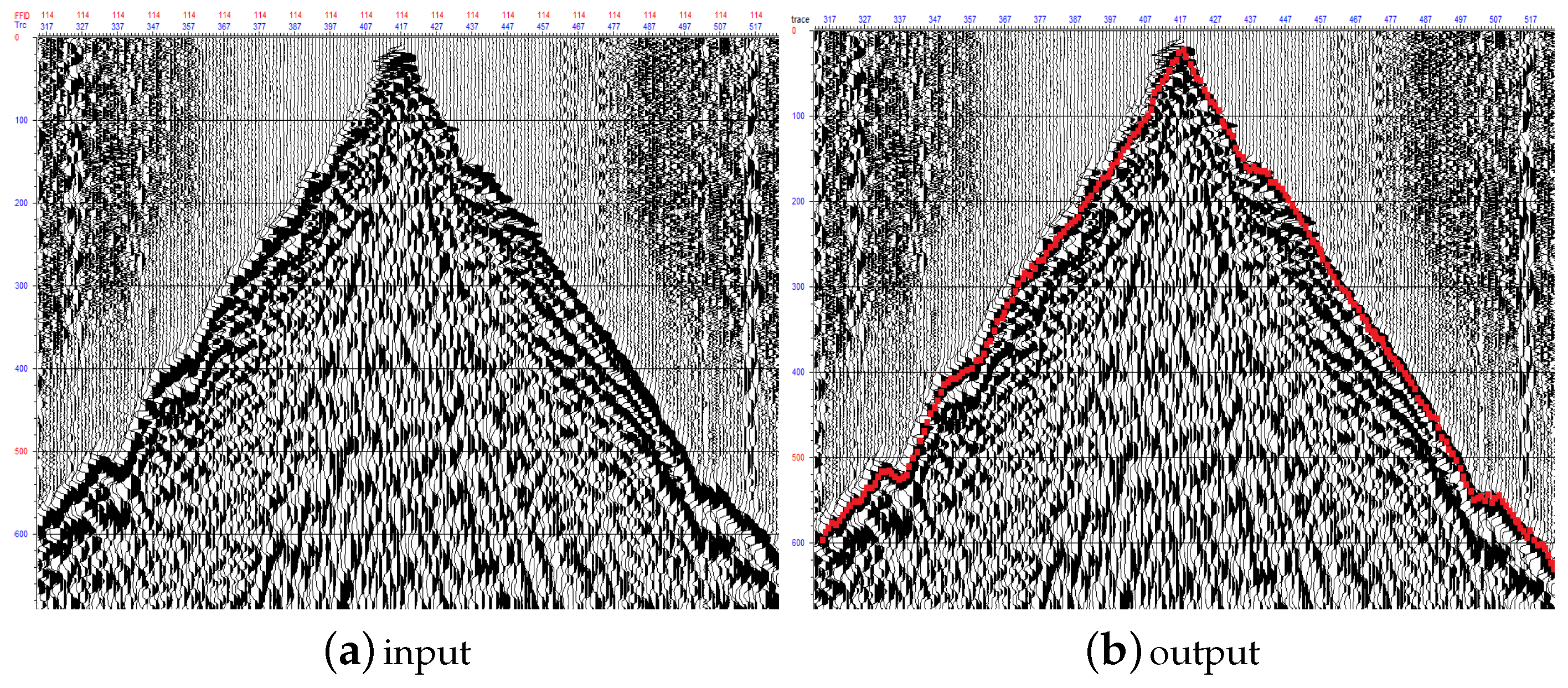
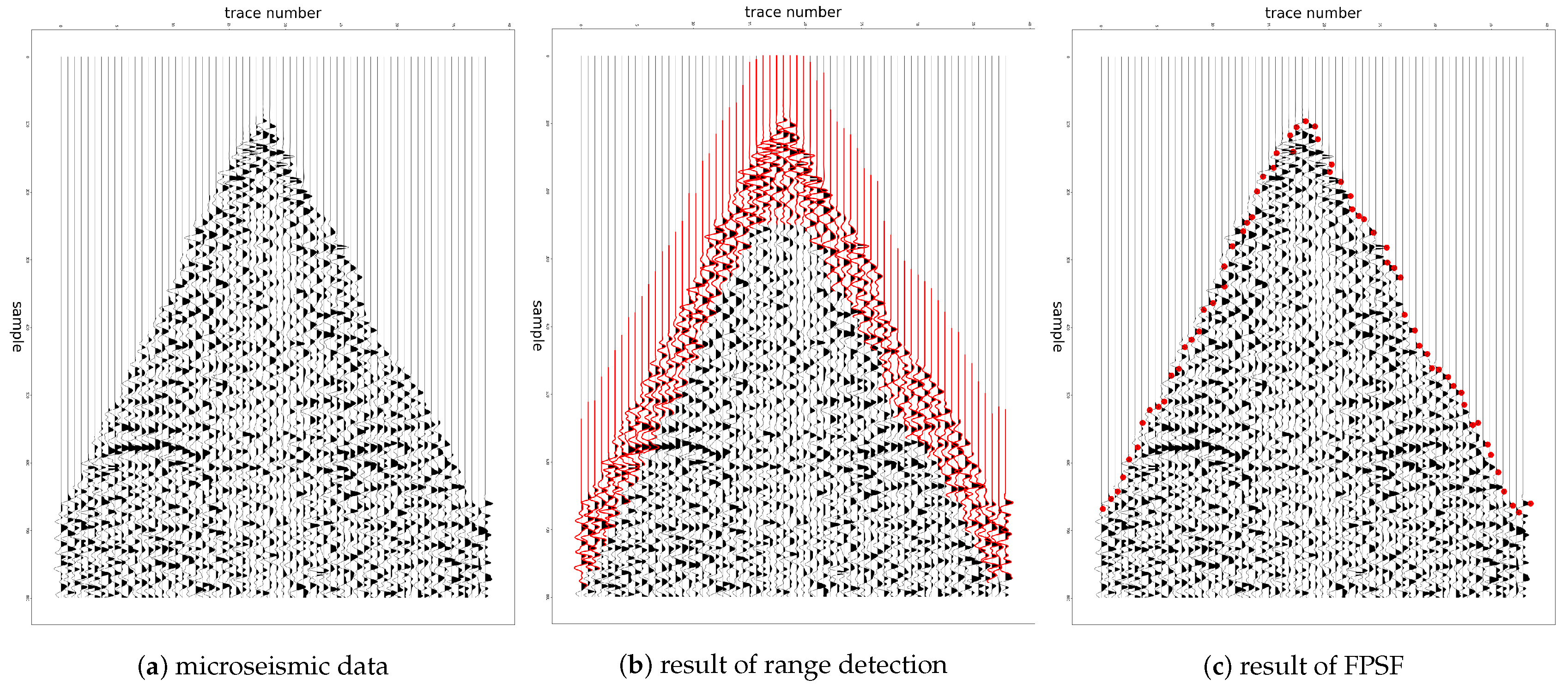
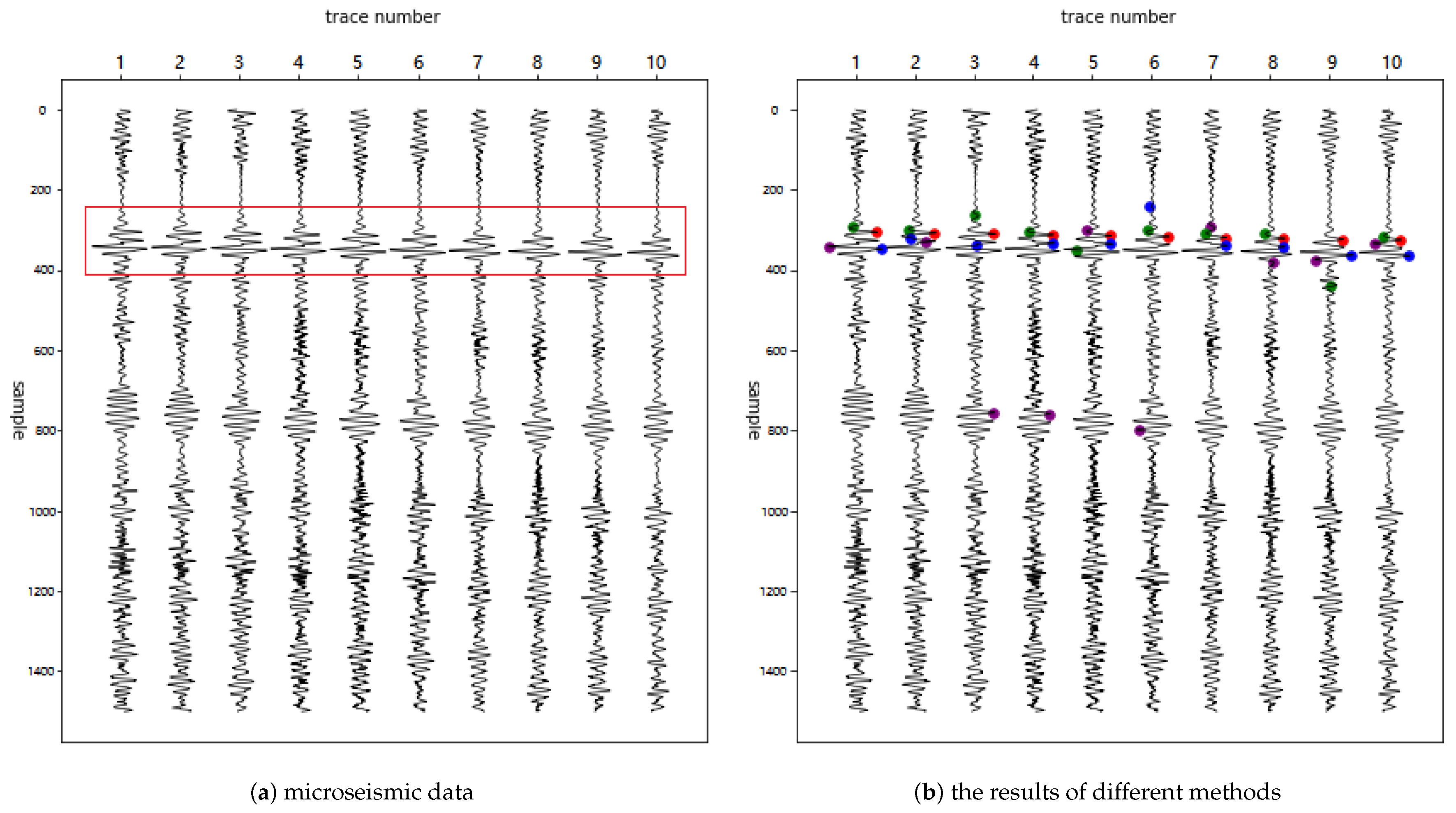
5. Experimental Results

This section shows the experimental results with two data sets.

Figure 3a shows the field microseismic data consists of 280 shots from $Xinjiang$, China. Every shot has about 400 traces and time sampling interval is 2 ms. Figure 3b shows the result of range detection. Figure 3c shows the result of FPSF.

Figure 4a shows the field microseismic data consists of 150 shots from $Sichuan$, China. Every shot has about 500 traces and time sampling interval is 2 ms. Figure 4b shows the result of range detection. Figure 4c shows the result of FPSF.

Figure 5a shows Xinjiang field microseismic data. Figure 5b shows the comparison of the difference among the values by the MCM method (purple spots), BNN method (blue spots), DC method (green spots) and FPSF (red spots).

Table 2. Accuracy comparison.

Data Sources (Data Length)	BNN	DC	MCM	FPSF
Xinjiang (300200)	$31.5\%$	$81\%$	$84\%$	$96.5\%$
Sichuan (160064)	$3.125\%$	$4.69\%$	$82.81\%$	$81.25\%$

shows the accuracy of each method for different data sets. We can find out that FPSF is more accurate than BNN, DC on the two data sets and MCM on one data set. In general, FPSF shows superiority over BNN, DC and MCM on the two data sets.

6. Conclusions

At the current stage of developments of artificial intelligence, we urgently need new theories applied to seismic exploration rather than sticking to the theory of seismic exploration itself. In this paper, we propose the first-arrival picking through sliding windows and fuzzy c-means (FPSF) algorithm. The biggest difference from the conventional methods that are currently available is that our method does not directly pick up the first-arrival travel times but determines a first-arrival range before picking. Combined with the characteristics of seismic data, we have improved some methods, such as particle swarm optimization and fuzzy c-means. Experiments with Xinjiang’s data set with 280 shots and Sichun’s data set with 150 shots show that the proposed method can significantly improve accuracy and stability. In the future, we will apply the idea of FPSF to other domains such as image processing.

References

1. Waheed, U.B.; Flagg, G.; Yarman, C.E. First-arrival traveltime tomography for anisotropic media using the adjoint-state method. Geophysics 2016, 81, R147–R155. [Google Scholar] [CrossRef]
2. Zelt, C.; Haines, S.; Powers, M.; Sheehan, J.; Rohdewald, S.; Link, C.; Hayashi, K.; Zhao, D.; Zhou, H.W.; Burton, B.; et al. Blind test of methods for obtaining 2-D near-surface seismic velocity models from first-arrival traveltimes. J. Environ. Eng. Geophys. 2013, 18, 183–194. [Google Scholar] [CrossRef]
3. Sun, M.Y.; Zhang, J.; Zhang, W. Alternating first-arrival traveltime tomography and waveform inversion for near-surface imaging. Geophysics 2017, 82, R245–R257. [Google Scholar] [CrossRef]
4. Zhu, X.H.; Valasek, P.; Roy, B.; Shaw, S.; Howell, J.; Whitney, S.; Whitmore, N.D.; Anno, P. Recent applications of turning-ray tomography. Geophysics 2008, 73, VE243–VE254. [Google Scholar] [CrossRef]
5. Kahrizi, A.; Hashemi, H. Neuron curve as a tool for performance evaluation of MLP and RBF architecture in first break picking of seismic data. J. Appl. Geophys. 2014, 108, 159–166. [Google Scholar] [CrossRef]
6. Yilmaz, Ö. Seismic Data Analysis: Processing, Inversion, and Interpretation of Seismic Data; Society of Exploration Geophysicists: Tulsa, OK, USA, 2001; Volume 1. [Google Scholar] [CrossRef]
7. An, S.; Hu, T.Y.; Peng, G.X. Three-Dimensional cumulant-based coherent integration method to enhance first-break seismic signals. IEEE Trans. Geosci. Remote Sens. 2017, 55, 2089–2096. [Google Scholar] [CrossRef]
8. Akram, J.; Eaton, D.W. A review and appraisal of arrival-time picking methods for downhole microseismic data. Geophysics 2016, 81, KS71–KS91. [Google Scholar] [CrossRef]
9. Li, Y.; Wang, Y.; Lin, H.B.; Zhong, T. First arrival time picking for microseismic data based on DWSW algorithm. J. Seismol. 2018, 22, 833–840. [Google Scholar] [CrossRef]
10. Hu, R.Q.; Wang, Y.C. A first arrival detection method for low SNR microseismic signal. Acta Geophys. 2018, 66, 945–957. [Google Scholar] [CrossRef]
11. Lan, H.Q.; Zhang, Z.J. A high-order fast-sweeping scheme for calculating first-arrival travel times with an trregular surface. Bull. Seismol. Soc. Am. 2013, 103, 2070–2082. [Google Scholar] [CrossRef]
12. Coppens, F. First arrival picking on common-offset trace collections for automatic estimation of static corrections. Geophys. Prospect. 1985, 33, 1212–1231. [Google Scholar] [CrossRef]
13. Al-Ghamdi, A.S. Automatic First Arrival Picking Using Energy Ratios; ProQuest: Ann Arbor, MI, USA, 2007. [Google Scholar]
14. Chen, M.; Li, Y.; Xie, J. A novel SVM-Based method for seismic first-arrival detecting. Appl. Mech. Mater. 2010, 29–32, 973–978. [Google Scholar] [CrossRef]
15. Sabbione, J.I.; Velis, D. Automatic first-breaks picking: New strategies and algorithms. Geophysics 2010, 75, V67–V76. [Google Scholar] [CrossRef]
16. Molyneux, J.B.; Schmitt, D.R. First-break timing: Arrival onset times by direct correlation. Geophysics 1999, 64, 1492–1501. [Google Scholar] [CrossRef]
17. McCormack, M.D.; Zaucha, D.E.; Dushek, D.W. First-break refraction event picking and seismic data trace editing using neural networks. Geophysics 1993, 58, 67–78. [Google Scholar] [CrossRef]
18. Zhu, D.; Li, Y.; Zhang, C. Automatic time picking for microseismic data based on a fuzzy c-means clustering algorithm. IEEE Geosci. Remote Sens. Lett. 2016, 13, 1900–1904. [Google Scholar] [CrossRef]
19. Mousa, W.A.; Al-Shuhail, A.A.; Al-Lehyani, A. A new technique for first-arrival picking of refracted seismic data based on digital image segmentation. Geophysics 2011, 76, V79–V89. [Google Scholar] [CrossRef]
20. Allen, R.V. Automatic earthquake recognition and timing from single traces. Bull. Seismol. Soc. Am. 1978, 68, 1521–1532. [Google Scholar]
21. Wong, J.; Han, L.J.; Bancroft, J.C.; Stewart, R.R. Automatic time-picking of first arrivals on noisy microseismic data. Can. Soc. Explor. Eeophys. Conf. Abstr. 2009, 1, 1–4. [Google Scholar]
22. Takanami, T.; Kitagawa, G. Estimation of the arrival times of seismic waves by multivariate time series model. Ann. Inst. Stat. Math. 1991, 43, 407–433. [Google Scholar] [CrossRef]
23. Boschetti, F.; Dentith, M.D.; List, R.D. A fractal-based algorithm for detecting first arrivals on seismic traces. Geophysics 1996, 61, 1095–1102. [Google Scholar] [CrossRef]
24. Tian, N.; Fan, T.G.; Hu, G.Y.; Zhang, R.W.; Zhou, J.N.; Le, J. The roles of the spatial regularization in seismic deconvolution. Acta Geod. Geophys. 2016, 51, 43–55. [Google Scholar] [CrossRef]
25. Bertrand, A.; MacBeth, C. Repeatability enhancement in deep-water permanent seismic installations: A dynamic correction for seawater velocity variations. Geophys. Prospect. 2005, 53, 229–242. [Google Scholar] [CrossRef]
26. Strong, S.; Hearn, S. Statics correction methods for 3D converted-wave (PS) seismic reflection. Explor. Geophys. 2017, 48, 237–245. [Google Scholar] [CrossRef]
27. Cox, M. Static Corrections for Seismic Reflection Surveys; Society of Exploration Geophysicists: Tulsa, OK, USA, 1999. [Google Scholar] [CrossRef]
28. Naus-Thijssen, F.M.J.; Goupee, A.J.; Vel, S.S.; Johnson, S.E. The influence of microstructure on seismic wave speed anisotropy in the crust: Computational analysis of quartz-muscovite rocks. Geophys. J. Int. 2011, 185, 609–621. [Google Scholar] [CrossRef]
29. Li, Q.H.; Jia, X.F. Generalized staining algorithm for seismic modeling and migration. Geophysics 2017, 82, T17–T26. [Google Scholar] [CrossRef]
30. Hatherly, P.J. A computer method for determining seismic first arrival times. Geophysics 1982, 47, 1431–1436. [Google Scholar] [CrossRef]
31. Fajaryanti, R.; Manik, H.M.; Purwanto, C. Application of multichannel seismic reflection method to measure temperature in Sulawesi Sea. IOP Conf. Ser. Earth Environ. Sci. 2018, 176, 012044. [Google Scholar] [CrossRef]
32. Wang, F.Y.; Zhao, C.B.; Feng, S.Y.; Ji, J.F.; Tian, X.F.; Wei, X.Q.; Li, Y.Q.; Li, J.C.; Hua, X.S. Seismogenic structure of the 2013 Lushan M (s) 7.0 earthquake revealed by a deep seismic reflection profile. Chin. J. Geophys. Chin. Ed. 2015, 58, 3183–3192. [Google Scholar]
33. Dunn, J.C. A fuzzy relative of the ISODATA process and its use in detecting compact well-separated clusters. J. Cybern. 1973, 3, 32–57. [Google Scholar] [CrossRef]
34. Bezdek, J.C. Pattern recognition with fuzzy objective function algorithms. Adv. Appl. Pattern Recognit. 1981, 22, 203–239. [Google Scholar]
35. Jia, Z.X.; Xia, Y.; Chen, Q.; Sun, Q.S.; Xia, D.S.; Feng, D.D. Fuzzy c-means clustering with weighted image patch for image segmentation. Appl. Soft Comput. 2012, 12, 1659–1667. [Google Scholar] [CrossRef]
36. Shafei, B.; Steidl, G. Segmentation of images with separating layers by fuzzy c-means and convex optimization. J. Vis. Commun. Image Represent. 2012, 23, 611–621. [Google Scholar] [CrossRef] [Green Version]
37. Szilágyi, L.; Szilágyi, S.M.; Benyó, Z. A modified FCM algorithm for fast segmentation of brain MR images. In Analysis and Design of Intelligent Systems using Soft Computing Techniques; Springer: Berlin/Heidelberg, Germany, 2007; pp. 119–127. [Google Scholar] [CrossRef]
38. Ahmed, M.N.; Yamany, S.M.; Mohamed, N.; Farag, A.A.; Moriarty, T. A modified fuzzy c-means algorithm for bias field estimation and segmentation of MRI data. IEEE Trans. Med. Imaging 2002, 21, 193–199. [Google Scholar] [CrossRef] [PubMed] [Green Version]
39. Bezdek, J.C.; Pal, S.K. Fuzzy Models for Pattern Recognition; IEEE Press: New York, NY, USA, 1992; Volume 56. [Google Scholar]
40. Kennedy, J. Particle swarm optimization. In Encyclopedia of Machine Learning; Springer: Boston, MA, USA, 2011; pp. 760–766. [Google Scholar] [CrossRef]
41. Ganguly, S.; Sahoo, N.C.; Das, D. Multi-objective particle swarm optimization based on;fuzzy-pareto-dominance for possibilistic planning of electrical;distribution systems incorporating distributed generation. Fuzzy Sets Syst. 2013, 213, 47–73. [Google Scholar] [CrossRef]
42. Tsekouras, G.E.; Tsimikas, J. On training RBF neural networks using input-output fuzzy clustering and particle swarm optimization. Fuzzy Sets Syst. 2013, 221, 65–89. [Google Scholar] [CrossRef]
43. Wang, G.G.; Guo, L.H.; Gandomi, A.H.; Hao, G.S.; Wang, H.Q. Chaotic krill herd algorithm. Inf. Sci. 2014, 274, 17–34. [Google Scholar] [CrossRef]
44. Wang, G.G.; Tan, Y. Improving metaheuristic algorithms with information feedback models. IEEE Trans. Cybern. 2017, 49, 542–555. [Google Scholar] [CrossRef] [PubMed]
45. Fang, Y.; Liu, Z.H.; Min, F. A PSO algorithm for multi-objective cost-sensitive attribute reduction on numeric data with error ranges. Soft Comput. 2017, 21, 7173–7189. [Google Scholar] [CrossRef]
46. Ding, S.C.; Hang, J.; Wei, B.L.; Wang, Q.J. Modelling of supercapacitors based on SVM and PSO algorithms. IET Electr. Power Appl. 2018, 12, 502–507. [Google Scholar] [CrossRef]
47. Keogh, E.; Chakrabarti, K.; Pazzani, M.; Mehrotra, S. Dimensionality reduction for fast similarity search in large time series databases. Knowl. Inf. Syst. 2001, 3, 263–286. [Google Scholar] [CrossRef]
48. Mousas, C.; Anagnostopoulos, C.N. Learning motion features for example-based finger motion estimation for virtual characters. 3D Res. 2017, 8, 25. [Google Scholar] [CrossRef]
49. Liu, H.; Xiao, G.F. Improved fuzzy clustering image segmentation algorithm based on particle swarm optimization. Comput. Eng. Appl. 2013, 49, 37–52. [Google Scholar] [CrossRef]
Figure 1. The framework of the FPSF algorithm (In the middle part, red indicates first-arrival intervals or initial clustering centers; In the right-top part, red indicates the first-arrival range; In the right-bottom part, red indicates first arrivals).
Mathematics 07 00221 g001
Figure 2. Field data and first-arrival travel times.
Mathematics 07 00221 g002
Figure 3. First arrivals picked by FPSF for field microseismic record. (a) field microseismic record; (b) the result of range detection; (c) the result of FPSF.
Mathematics 07 00221 g003
Figure 4. First arrivals picked by FPSF for field microseismic record. (a) field microseismic record; (b) the result of range detection; (c) the result of FPSF.
Mathematics 07 00221 g004
Figure 5. First arrivals picked by FPSF for field microseismic record. (a) field microseismic record; (b) the result of different methods: MCM (purple), BNN (blue), DC (green), FPSF (red).
Mathematics 07 00221 g005