Stability Analysis of Singly Diagonally Implicit Block Backward Differentiation Formulas for Stiff Ordinary Differential Equations

Abstract

In this research, a singly diagonally implicit block backward differentiation formulas (SDIBBDF) for solving stiff ordinary differential equations (ODEs) is proposed. The formula reduced a fully implicit method to lower triangular matrix with equal diagonal elements which will results in only one evaluation of the Jacobian and one LU decomposition for each time step. For the SDIBBDF method to have practical significance in solving stiff problems, its stability region must at least cover almost the whole of the negative half plane. Step size restriction of the proposed method have to be considered in order to ensure stability of the method in computing numerical results. Efficiency of the SDIBBDF method in solving stiff ODEs is justified when it managed to outperform the existing methods for both accuracy and computational time.

1. Introduction

Many problems in engineering, physical and social sciences are reduced to quantifiable form through mathematical modelling involving systems of ordinary differential equations (ODEs). These problems sometimes exhibit a phenomenon known as stiffness. It associates with components that are decaying at widely differing rates. For this article, our main concern is the linear system of first order stiff ODEs of the form

$$y^{\prime }\left(x\right)=f(x,y),y\left(a\right)=\mu ,x\in [a,b],$$

(1)

where $y^T=(y_1\left(x\right),y_2\left(x\right),\dots ,y_d\left(x\right))$, $f^T=(f_1\left(x\right),f_2\left(x\right),\dots ,f_d\left(x\right))$ and ${\mu }^T=({\mu }_1\left(x\right),{\mu }_2\left(x\right),\dots ,{\mu }_d\left(x\right))$. Equation (1) is said to be linear if $f(x,y)=A\left(x\right)y+\Phi \left(x\right)$, where $A\left(x\right)$ is a constant $d\times d$ matrix and $\Phi \left(x\right)$ is an $d$-dimensional vector.

There are various definitions of stiffness that exist in the literature. However, we consider the one given by [1] which stated that the linear system (1) is said to be stiff if

• $Re\left({\lambda }_i\right)<0$, $i=1,2,\dots ,d$ and
• $\underset{i}{\max }\left|Re\left({\lambda }_i\right)\right|\gg \underset{i}{\min }\left|Re\left({\lambda }_i\right)\right|$, where ${\lambda }_i$ are the eigenvalues of A and the ratio $S=\frac{\underset{i}{\max }\left|Re\left({\lambda }_i\right)\right|}{\underset{i}{\min }\left|Re\left({\lambda }_i\right)\right|}$ is called the stiffness ratio.

Most realistic stiff systems do not have analytical solutions, hence a numerical approach have to be used [2]. An exact solution of (1) can be approximated by using either the one-step method or the linear multistep method (LMM). Euler’s is the simplest form of one-step method whereas the Runge-Kutta (RK) method is the most famous family under this class. These methods use the solution of current point, $y_n$, as initial value to compute solution at the next point, $y_{n+1}$.

On the contrary, LMM uses information from the previous points to calculate the next values. Adams and BDF method are examples of families under the LMM. A classical approach for numerical methods in finding an approximation of $y_{n+1}$ at the point $x_{n+1}$ is computed one step at a time.

In order to accelerate the computational process, block method is introduced with the idea of producing simultaneously k-blocks where each block contains r-point approximation, $y_{n+1},y_{n+2},\dots ,y_{n+r}$, at each iteration of the algorithm. For the multistep block method, points from the previous block calculated are used in generating approximation solutions for the new block. The block method is first proposed by [3] which is later extended by several researchers such as [4,5,6]. A modified block by Adams method for higher order ODEs had been discussed by [7] followed by [8] for solving nonstiff higher order ODEs.

As for stiff ODEs, fixed coefficients BBDF introduced by [9] had proved to optimize performance in both accuracy and computational time when solving stiff problems. Not only that, but the method also managed to outperform the non-block variable step variable order BDF (VSVOBDF) method by [10] (as cited in [9]). Numbers of improvement had been made to the original BBDF method, one of them is the diagonally implicit 2-point BBDF (DI2BBDF) method by [11] that gives better accuracy for high dimension problem of ODEs than the BBDF method. The method is derived based on the motivation by [12] which defined the diagonally implicit as the method with its coefficients of the upper-diagonal (read: lower triangular) entries are zero.

Over the years, conventional RK methods evolutionized to form the best solver for ODEs. The commonly improved RK methods involved an implementation of singly diagonally implicit properties which had proved to produce better computational time when compared with the existing methods. Among the initial works on the singly diagonally implicit RK (SDIRK) method is [13], which defined a singly diagonally implicit as a method with equal diagonal elements, ${\alpha }_{ii}=\gamma$, as shown in the Butcher tableau below.

$c_1$	$\gamma$	0	⋯	0
$c_2$	${\alpha }_{21}$	$\gamma$	⋯	0
⋮	⋮	⋮		⋮
$c_n$	${\alpha }_{n1}$	${\alpha }_{n2}$	⋯	$\gamma$
	$b_1$	$b_2$	⋯	$b_n$

The proposed problem of stiff ODEs is also considered by [14] through Newton-type iterations that solve for linear systems at each stage with coefficient matrix of the form $I-h{\alpha }_{ii}\frac{\partial f}{\partial y}$. Based on [15], singly implicit RK is a transformed method whose RK matrix has just one real $s$-fold eigenvalue. If we have ${\alpha }_{ii}=\gamma$, then the class of diagonally implicit RK (DIRK) is called SDIRK methods [16].

The definition of SDIRK by Norsett is further discussed by [17,18,19] in their research. As summarized by [20], when having the lower triangular matrix with equal diagonal elements, the stored LU-factorization of a single such matrix can be used repeatedly. Hence, only one evaluation of the Jacobian and one LU decomposition will be needed for each time step. By having these properties, degree of implicitness can also be reduced as it involved less computational process which will results in less execution time [21].

Therefore, developing the SDIBBDF method involves the hybrid process of implementing qualities from SDIRK method to block multistep method. As we know, both methods are of different families hence, our main concern is the compatibility of the derived method to solve for stiff ODEs. Derivation of the SDIBBDF method is shown in the next section.

2. Research Methodology

2.1. Derivation of 2-Point SDIBBDF Method

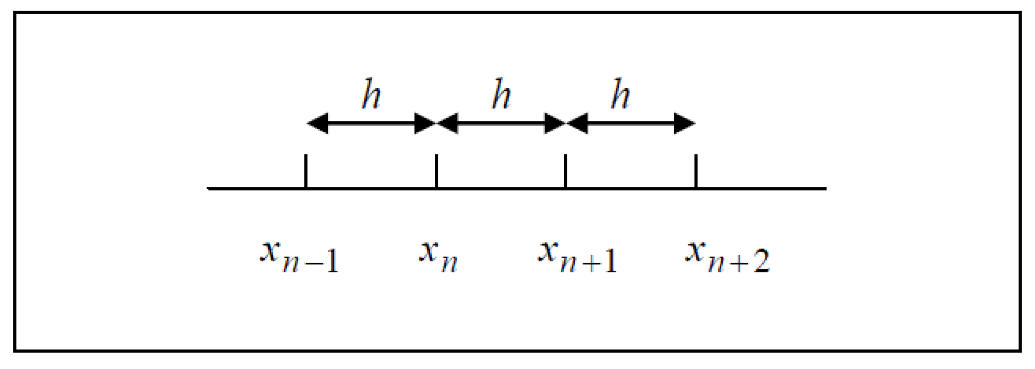
Our main objective is to develop a method that capable of computing two solutions, $y_{n+1}$ and $y_{n+2}$, simultaneously in less expensive environment with accurate approximation to the exact solution of stiff ODEs. The idea is illustrated as shown in Figure 1.

Points $x_{n-1}$ and $x_n$ are the back values used to evaluate solutions of future points, $x_{n+1}$ and $x_{n+2}$, with constant step size. Hence, we proposed the 2-point SDIBBDF method of order 2 with

$$\sum _{j=0}^{k+s-2}{\alpha }_{s,j}{y}_{n+j}=h{\beta }_{s,k+s-2}{f}_{n+s}$$

(2)

where $k=2$, and $s=1,2$ for points $y_{n+1}$ and $y_{n+2}$ respectively with ${\alpha }_{ii}=\gamma$, as referred in [13]. We consider the linear difference operator for block multistep method (2) as

$$L_s(y\left(x\right):h)=\sum _{j=0}^{k+s-2}({\alpha }_{s,j}y(x+jh)-h{\beta }_{s,k+s-2}y(x+sh).$$

(3)

Equation (3) is expanded by using the Taylor series, and the terms of derivative y are collected to produce

$$L_s(y\left(x\right):h)=C_{0}y\left(x\right)+C_1{y}^{\prime }\left(x\right)+\dots +C_q{y}^q\left(x\right)+\dots .$$

(4)

The constant $C_q$ is defined as

$$\begin{array}{cc}\hfill C_0& =\sum _{j=0}^{k+s-2}{\alpha }_j,\hfill \\ \hfill C_1& =\sum _{j=0}^{k+s-2}j{\alpha }_j-{\beta }_j,\hfill \\ \hfill ⋮\\ \hfill C_q& =\left[\frac{1}{q!}\sum _{j=0}^{k+s-2}{j}^q{\alpha }_j-\frac{1}{(q-1)!}\sum _{j=2}^{k+s-2}{j}^{q-1}{\beta }_j\right],q=2,3,\dots .\hfill \end{array}$$

(5)

Since the SDIBBDF method proposed is of order 2, $k=3$ and $q=2$ are substituted into Equation (4) to get

$$\begin{array}{cc}\hfill C_0& =\left[\begin{array}{c}{\alpha }_{1,-1}{\alpha }_{1,0}\gamma 0\\ {\alpha }_{2,-1}{\alpha }_{2,0}{\alpha }_{2,1}\gamma \end{array}\right]=0,\hfill \\ \hfill C_1& =\left[\begin{array}{c}{\alpha }_{1,0}2\gamma 0-{\beta }_{1,2}0\\ {\alpha }_{2,0}2{\alpha }_{2,1}3\gamma 0-{\beta }_{2,3}\end{array}\right]=0,\hfill \\ \hfill C_2& =\left[\begin{array}{c}{\displaystyle \frac{1}{2}}{\alpha }_{1,0}2\gamma 0-2{\beta }_{1,2}0\\ {\displaystyle \frac{1}{2}}{\alpha }_{2,0}2{\alpha }_{2,1}{\displaystyle \frac{9}{2}}\gamma 0-3{\beta }_{2,3}\end{array}\right]=0,\hfill \end{array}$$

(6)

By using MAPLE, Equation (6) is solved simultaneously, and the coefficients obtained are substituted into Equation (2). The formula derived is rewritten in matrices form as shown below:

$$\left[\begin{array}{c}{\displaystyle \frac{1}{2}}-2\\ 0{\displaystyle \frac{1}{2}}\end{array}\right]\left[\begin{array}{c}{y}_{n-1}\\ y_n\end{array}\right]+\left[\begin{array}{c}{\displaystyle \frac{3}{2}}0\\ -2{\displaystyle \frac{3}{2}}\end{array}\right]\left[\begin{array}{c}{y}_{n+1}\\ y_{n+2}\end{array}\right]=h\left[\begin{array}{c}{\beta }_{1,2}0\\ 0{\beta }_{2,3}\end{array}\right]\left[\begin{array}{c}{f}_{n+1}\\ f_{n+2}\end{array}\right].$$

(7)

Therefore, the general formula of 2-point SDIBBDF method of order 2 is as follows:

$$\begin{array}{cc}\hfill y_{n+1}& ={\displaystyle \frac{1}{3}}{y}_{n-1}+{\displaystyle \frac{4}{3}}{y}_n+{\displaystyle \frac{2}{3}}h{f}_{n+1},\hfill \\ \hfill y_{n+2}& ={\displaystyle \frac{1}{3}}{y}_n+{\displaystyle \frac{4}{3}}{y}_{n+1}+{\displaystyle \frac{2}{3}}h{f}_{n+2}.\hfill \end{array}$$

(8)

In the next subsection, we will discuss on stability of the derived SDIBBDF method.

2.2. Stability Analysis

One of the practical characteristics for a method to be useful is that it must have a region of absolute stability.

Definition 1.

The LMM in Equation (1) is said to be absolutely stable in a region R for a given H if and only if for that H, all the roots, $r_s=r_s\left(H\right)$ of the stability polynomial of the linear k-step method, $\pi (r,H)=\rho \left(r\right)-H\varphi \left(r\right)$, satisfy $|r_s|<1$, $s=1,2,\dots ,k$ where $H=h\lambda$ and $\rho \left(r\right)$ and $\varphi \left(r\right)$ are the first and second characteristic polynomials respectively. Otherwise the method is said to be absolutely unstable.

In order to analyse the stability properties of the proposed method, a stability graph of the SDIBBDF method has to be constructed. First, characteristic polynomial of the method is determined by referring to the following statement.

Definition 2.

The characteristic polynomial of LMM in Equation (1) assumes

$$\pi (r,h\lambda )=\rho \left(r\right)-h\lambda \varphi \left(r\right)=0,$$

where $H=h\lambda$ and $\lambda ={\displaystyle \frac{\partial f}{\partial y}}$ is complex.

By applying the Dahlquist test equation of

$$\begin{array}{cc}{y}^{\prime }\hfill & =f(x,y)\hfill \\ & =\lambda y\hfill \end{array}$$

(9)

to Equation (7), we get

$$\begin{array}{c}\left[\begin{array}{cc}1-{\displaystyle \frac{2}{3}}H& 0\\ -{\displaystyle \frac{4}{3}}& 1-{\displaystyle \frac{2}{3}}H\end{array}\right]\left[\begin{array}{c}{y}_{n+1}\\ y_{n+2}\end{array}\right]=\left[\begin{array}{cc}-{\displaystyle \frac{1}{3}}& {\displaystyle \frac{4}{3}}\\ 0& -{\displaystyle \frac{1}{3}}\end{array}\right]\left[\begin{array}{c}{y}_{n-1}\\ y_n\end{array}\right]\end{array}$$

(10)

which is equivalent to

$$A{Y}_m=B{Y}_{m-1},$$

where A and B are properly chosen $r\times r$ matrix coefficients and m represents the block number.

We consider $\rho \left(t\right)=det(At-B)$ as the first characteristic polynomial of the SDIBBDF method. By substituting Equation (10) into $\rho \left(t\right)$,

$$\begin{array}{c}\rho \left(t\right)=det\left[\begin{array}{cc}\left(1-{\displaystyle \frac{2}{3}}H\right)t+{\displaystyle \frac{1}{3}}& -{\displaystyle \frac{4}{3}}\\ -{\displaystyle \frac{4}{3}}t& \left(1-{\displaystyle \frac{2}{3}}H\right)t+{\displaystyle \frac{1}{3}}\end{array}\right].\end{array}$$

(11)

Based on Definition 2, when we solve for $\rho \left(t\right)=0$, stability polynomial, $R\left(H\right)$, of Equation (8) is obtained.

$$R\left(H\right)={\displaystyle \frac{4}{9}}{t}^2{H}^2-{\displaystyle \frac{4}{3}}{t}^{2}H+t^2-{\displaystyle \frac{4}{9}}tH-{\displaystyle \frac{10}{9}}t+{\displaystyle \frac{1}{9}}.$$

(12)

In order to determine zero stability of the SDIBBDF method, we refer to the following definition.

Definition 3.

The LMM in (1) is said to be zero-stable if no root of the first characteristic polynomial, $\rho \left(\zeta \right)$, has modulus greater than one, and if every root with modulus one is simple.

Solving $R\left(H\right)=0$ yields the following roots:

$$t=0,1.$$

(13)

Therefore, Equation (13) proved that the SDIBBDF method is zero stable.

To plot $R\left(H\right)$, we let for each value of H, R is a complex number. Boundary of the stability region is the set of all H such that $R\left(H\right)$ is on the unit circle of

$$R\left(H\right)=e^{i\theta },$$

(14)

for some $\theta \in [0,2\pi ]$. Equation (14) is expanded for various value of $\theta$ in steps of $\frac{2\pi }{n}$ from 0 to $2\pi$.

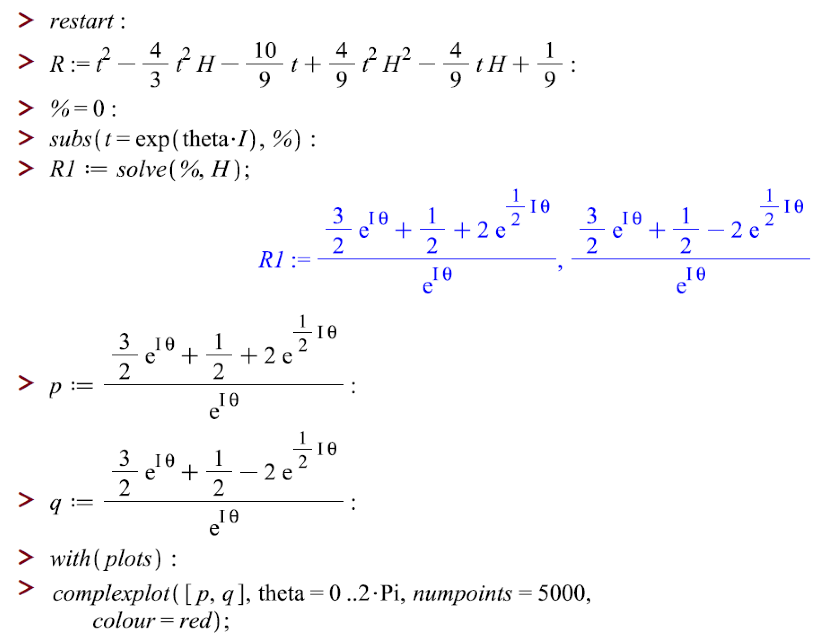
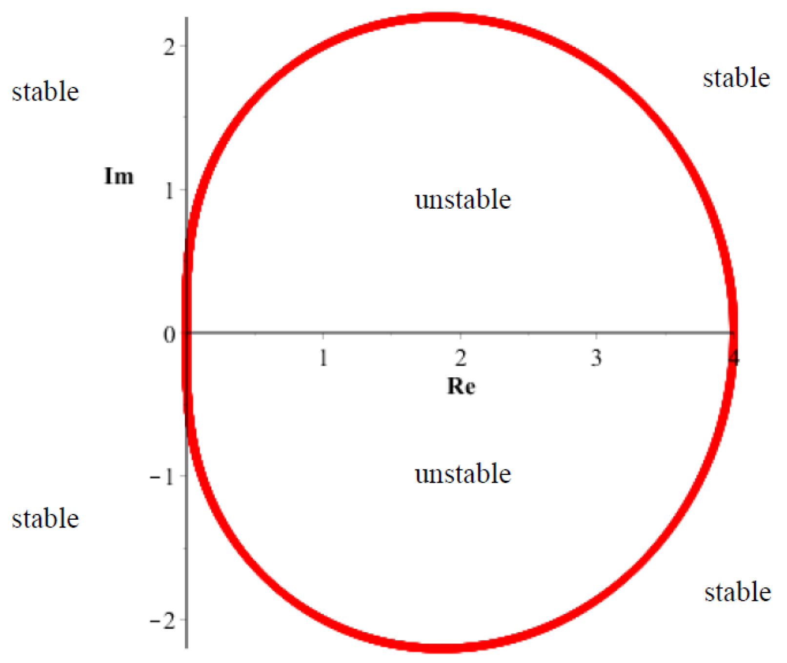
Next, the points are plotted by using MAPLE as shown in Figure 2 while Figure 3 represents the output which is the stability graph of 2-point SDIBBDF method.

By referring to [22] a method is suitable for solving stiff problems because of its A-stability property as reviewed in the following statement.

Definition 4.

A numerical method is said to be A-stable if its region of absolute stability contains the whole left-hand half-plane, $Re\left(h\lambda \right)<0$.

As observed in Figure 3, the area inside the closed region is unstable whereas the stable part lies outside the region. Coincide with Definition 4, we can conclude that the 2-point SDIBBDF method of order 2 is A-stable.

Suppose that the following definition is applied.

Definition 5.

The LMM in Equation (1) is said to have region of absolute stability, ${\Re }_A$, where ${\Re }_A$ is a region of the complex $\widehat{h}$-plane, if it is absolutely stable for all $\widehat{h}\in {\Re }_A$. The intersection with real axis is called the interval of absolute stability.

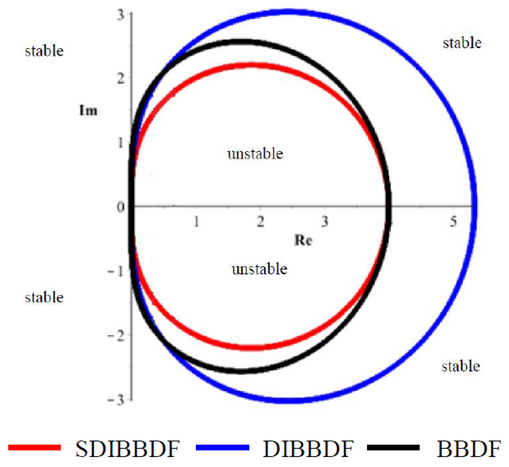
For SDIBDDF method, its interval of absolute stability is $4<H<0$. Comparison in terms of stability region is made between the proposed method, fully implicit BBDF by [9] and DIBBDF method by [11] as shown in Figure 4.

Analysis on Figure 4 concludes that the unstable region of the proposed method is smaller when compared with the other methods. Interval of the unstable area for each method is presented in

Table 1. Interval of unstable area on real and imaginary axis.

METHOD	Re	Im
SDIBBDF	$[0,3.99]$	$[-2.20,2.19]$
DIBBDF	$[0,5.33]$	$[-3.03,3.01]$
BBDF	$[0,3.99]$	$[-2.57,2.55]$

.

From the table shown, it is noted that the unstable area of DIBBDF method is wider followed by the BBDF and SDIBBDF method. This proved that the SDIBBDF method has wider stability area than the comparing methods.

2.3. Step Size Restriction

As stated in Definition 1, an LMM is said to be absolutely stable when $\left|R\right(H\left)\right|<1$, otherwise it is unstable. There are two parameters involved, h and $\lambda$, but it is only their product, H, that needs to be taken into accounts.

By solving $\left|R\right(H\left)\right|<1$, we found that the SDIBBDF method is stable everywhere except when $H\in [0,4]$. However, h must lies within a certain range in order for the SDIBBDF method to be stable. By substituting endpoint of the interval into characteristic polynomial in Equation (12), we obtain

$$\epsilon =7.075600000H^2-23.00013333H+11.59787778.$$

(15)

Next, Equation (15) is presented in the form of $\left|\epsilon \right|<1$ which equal to

$$|7.075600000H^2-23.00013333H+11.59787778|<1.$$

(16)

Solving Equation (16) yields

$$\left|H\right|<0.6240609349.$$

Please note that $H=h\lambda$,

$$h<\left|{\displaystyle \frac{0.6240609349}{\lambda }}\right|.$$

(17)

Thus, Equation (17) is the step size restriction of SDIBBDF method. By taking an example of a stiff ODEs with eigenvalue, $\lambda =-100$,

$$h<\left|{\displaystyle \frac{0.6240609349}{-100}}\right|,$$

the suitable step size for solving the problem must be

$$h<0.006240609349.$$

If we take $h>0.006240609349$, the method will be unstable therefore, numerical solutions with large maximum error is produced.

3. Numerical Results

In the previous section, we claimed that the proposed method is A-stable hence, suitable for solving stiff problems. To validate this finding, we tested the SDIBBDF method to solve for single and system of stiff ODEs. Efficiency of the method is measured in terms of its accuracy and execution time.

Accuracy is analysed based on the maximum error,

$$MAXE=\underset{1\le i\le T}{max}(\underset{1\le i\le N}{max}{\left(erro{r}_i\right)}_t),$$

(18)

where T is the total number of steps and N is the number of equations. By considering the error as

$${\left(erro{r}_i\right)}_t=|{\left(y_i\right)}_t-{\left(y\left(x_i\right)\right)}_t|,$$

with $y_i$ and $y\left(x_i\right)$ are the approximate and exact solutions of Equation (8) respectively.

The following notations are used

SDIBBDF	:	Singly diagonally implicit BBDF method
DIBBDF	:	Diagonally implicit BBDF method by [23]
BBDF	:	BBDF method by [24]
ode15s	:	VSVO solver based on the numerical differentiation formulas (NDFs)
ode23s	:	modified Rosenbrock formula of order 2
h	:	step size
MAXE	:	maximum error
TIME	:	computational time

To verify performance of the methods, the following test problems of stiff ODEs are solved.

Test Problem 1

$$\begin{array}{cc}\hfill y^{\prime }=-20y+20sinx+cosx,& \hfill \hspace{1em}\hspace{1em}\hspace{1em}y\left(0\right)=1,0\le x\le 2\end{array}$$

Exact solution:

$$\begin{array}{c}\hfill y\left(x\right)=sinx+e^{-20x},\end{array}$$

Eigenvalue: $\lambda =-20$,

Source: [25].

Test Problem 2

$$\begin{array}{cc}\hfill y^{\prime }=100(sinx-y),& \hfill \hspace{1em}\hspace{1em}\hspace{1em}y\left(0\right)=0,0\le x\le 3\end{array}$$

Exact solution:

$$\begin{array}{c}\hfill y\left(x\right)={\displaystyle \frac{sinx-0.01cosx+0.01e^{-100x}}{1.0001}},\end{array}$$

Eigenvalue: $\lambda =-100$,

Source: [22].

Test Problem 3

$$\begin{array}{ccc}\hfill y_1^{\prime }& =32y_1+66y_2+{\displaystyle \frac{2}{3}}x+{\displaystyle \frac{2}{3}},\hfill & \hspace{1em}\hspace{1em}\hspace{1em}{y}_1\left(0\right)={\displaystyle \frac{1}{3}},0\le x\le 1,\hfill \\ \hfill y_2^{\prime }& =-66y_1-133y_2-{\displaystyle \frac{1}{3}}x-{\displaystyle \frac{1}{3}},\hfill & \hspace{1em}\hspace{1em}\hspace{1em}{y}_1\left(0\right)={\displaystyle \frac{1}{3}},\hfill \end{array}$$

Exact solution:

$$\begin{array}{cc}\hfill y_1\left(x\right)& ={\displaystyle \frac{2}{3}}x+{\displaystyle \frac{2}{3}}{e}^{-x}-{\displaystyle \frac{1}{3}}{e}^{-100x},\hfill \\ \hfill y_2\left(x\right)& =-{\displaystyle \frac{1}{3}}x-{\displaystyle \frac{1}{3}}{e}^{-x}+{\displaystyle \frac{2}{3}}{e}^{-100x},\hfill \end{array}$$

Eigenvalues: $\lambda =-100,-1$,

Source: [25].

Test Problem 4

$$\begin{array}{ccc}\hfill y_1^{\prime }& =-y_1+95y_2,\hfill & \hspace{1em}\hspace{1em}\hspace{1em}{y}_1\left(0\right)=1,0\le x\le 10,\hfill \\ \hfill y_2^{\prime }& =-y_1-97y_2,\hfill & \hspace{1em}\hspace{1em}\hspace{1em}{y}_2\left(0\right)=1,\hfill \end{array}$$

Exact solution:

$$\begin{array}{cc}\hfill y_1\left(x\right)& ={\displaystyle \frac{1}{47}}\left(95e^{-2x}-48e^{-96x}\right),\hfill \\ \hfill y_2\left(x\right)& ={\displaystyle \frac{1}{47}}\left(48e^{-96x}-e^{-2x}\right),\hfill \end{array}$$

Eigenvalues: $\lambda =-1000,-1$,

Source: [26].

Test Problem 5

$$\begin{array}{ccc}\hfill y_1^{\prime }& =-21y_1+19y_2-20y_3,\hfill & \hspace{1em}\hspace{1em}\hspace{1em}{y}_1\left(0\right)=1,0\le x\le 10,\hfill \\ \hfill y_2^{\prime }& =19y_1-21y_2+20y_3,\hfill & \hspace{1em}\hspace{1em}\hspace{1em}{y}_2\left(0\right)=0,\hfill \\ \hfill y_3^{\prime }& =40y_1-40y_2-40y_3,\hfill & \hspace{1em}\hspace{1em}\hspace{1em}{y}_3\left(0\right)=-1,\hfill \end{array}$$

Exact solution:

$$\begin{array}{cc}\hfill y_1\left(x\right)& =0.5\left[e^{-2x}+e^{-40x}\left(\cos 40x+\sin 40x\right)\right],\hfill \\ \hfill y_2\left(x\right)& =0.5\left[e^{-2x}-e^{-40x}\left(\cos 40x+\sin 40x\right)\right],\hfill \\ \hfill y_3\left(x\right)& =2e^{-40x}\left(-{\displaystyle \frac{1}{2}}\cos 40x+{\displaystyle \frac{1}{2}}\sin 40x\right),\hfill \end{array}$$

Eigenvalues: $\lambda =-40-40i,-40+40i,-2$,

Source: [1].

Table 2. Numerical results for test problem 1.

h	Method	Maxe	Time
	SDIBBDF	$4.17749\times {10}^{-2}$	$1.89443\times {10}^{-6}$
	DIBBDF	$9.19710\times {10}^{-2}$	$5.74779\times {10}^{-5}$
${10}^{-2}$	BBDF	$7.82684\times {10}^{-2}$	$6.11443\times {10}^{-5}$
	ode15s	$8.36909\times {10}^{-3}$	-
	ode23s	$4.07991\times {10}^{-3}$	-
	SDIBBDF	$4.94771\times {10}^{-6}$	$2.10183\times {10}^{-5}$
	DIBBDF	$1.46293\times {10}^{-3}$	$1.67354\times {10}^{-3}$
${10}^{-4}$	BBDF	$1.46435\times {10}^{-3}$	$3.76579\times {10}^{-3}$
	ode15s	$1.66322\times {10}^{-4}$	-
	ode23s	$1.83868\times {10}^{-4}$	-
	SDIBBDF	$4.99893\times {10}^{-10}$	$1.36298\times {10}^{-3}$
	DIBBDF	$1.47125\times {10}^{-5}$	$9.98032\times {10}^{-2}$
${10}^{-6}$	BBDF	$1.47126\times {10}^{-5}$	$1.07378\times {10}^{-1}$
	ode15s	$2.75074\times {10}^{-6}$	-
	ode23s	$1.25088\times {10}^{-5}$	-
	SDIBBDF	$4.97015\times {10}^{-10}$	$1.53342\times {10}^{-1}$
	DIBBDF	$1.47131\times {10}^{-7}$	$7.19868\times {10}^0$
${10}^{-8}$	BBDF	$1.47012\times {10}^{-7}$	$7.57031\times {10}^0$
	ode15s	$2.75074\times {10}^{-6}$	-
	ode23s	$1.25548\times {10}^{-5}$	-

,

Table 3. Numerical results for test problem 2.

h	Method	Maxe	Time
	SDIBBDF	$5.50135\times {10}^{-3}$	$1.17163\times {10}^{-7}$
	DIBBDF	$9.11949\times {10}^0$	$7.40632\times {10}^{-5}$
${10}^{-2}$	BBDF	$7.32490\times {10}^{-4}$	$8.05945\times {10}^{-5}$
	ode15s	$1.21111\times {10}^{-4}$	-
	ode23s	$1.70139\times {10}^{-3}$	-
	SDIBBDF	$1.20673\times {10}^{-6}$	$3.11372\times {10}^{-6}$
	DIBBDF	$7.14971\times {10}^{-5}$	$3.70624\times {10}^{-3}$
${10}^{-4}$	BBDF	$7.18301\times {10}^{-5}$	$6.91835\times {10}^{-3}$
	ode15s	$3.20516\times {10}^{-6}$	-
	ode23s	$3.75006\times {10}^{-5}$	-
	SDIBBDF	$1.24891\times {10}^{-10}$	$1.59917\times {10}^{-4}$
	DIBBDF	$7.35527\times {10}^{-7}$	$2.47110\times {10}^{-1}$
${10}^{-6}$	BBDF	$7.35563\times {10}^{-7}$	$7.47109\times {10}^{-1}$
	ode15s	$1.66215\times {10}^{-6}$	-
	ode23s	$2.61572\times {10}^{-6}$	-
	SDIBBDF	$1.23007\times {10}^{-10}$	$2.62004\times {10}^{-1}$
	DIBBDF	$7.35736\times {10}^{-9}$	$3.64344\times {10}^0$
${10}^{-8}$	BBDF	$7.35729\times {10}^{-9}$	$4.69932\times {10}^0$
	ode15s	$1.66215\times {10}^{-6}$	-
	ode23s	$2.62933\times {10}^{-6}$	-

,

Table 4. Numerical results for test problem 3.

h	Method	Maxe	Time
	SDIBBDF	$6.17982\times {10}^{-1}$	$7.86625\times {10}^{-6}$
	DIBBDF	$4.67257\times {10}^0$	$2.78780\times {10}^{-4}$
${10}^{-2}$	BBDF	$1.21585\times {10}^{-2}$	$4.03164\times {10}^{-4}$
	ode15s	$3.94538\times {10}^{-3}$	-
	ode23s	$1.56018\times {10}^{-3}$	-
	SDIBBDF	$8.04397\times {10}^{-5}$	$1.16277\times {10}^{-5}$
	DIBBDF	$4.76597\times {10}^{-3}$	$1.31756\times {10}^{-3}$
${10}^{-4}$	BBDF	$4.78817\times {10}^{-3}$	$4.48201\times {10}^{-3}$
	ode15s	$5.94372\times {10}^{-5}$	-
	ode23s	$8.46852\times {10}^{-5}$	-
	SDIBBDF	$8.32566\times {10}^{-9}$	$5.79741\times {10}^{-3}$
	DIBBDF	$4.90299\times {10}^{-5}$	$6.79440\times {10}^{-1}$
${10}^{-6}$	BBDF	$4.90323\times {10}^{-5}$	$8.49183\times {10}^{-1}$
	ode15s	$2.63297\times {10}^{-6}$	-
	ode23s	$1.09101\times {10}^{-5}$	-
	SDIBBDF	$3.79303\times {10}^{-9}$	$3.60277\times {10}^{-1}$
	DIBBDF	$4.90438\times {10}^{-7}$	$7.80285\times {10}^0$
${10}^{-8}$	BBDF	$4.90444\times {10}^{-7}$	$9.73183\times {10}^0$
	ode15s	$2.63297\times {10}^{-6}$	-
	ode23s	$1.09756\times {10}^{-5}$	-

,

Table 5. Numerical results for test problem 4.

h	Method	Maxe	Time
	SDIBBDF	$1.29000\times {10}^2$	$9.18958\times {10}^{-6}$
	DIBBDF	$9.88705\times {10}^{19}$	$5.24785\times {10}^{-4}$
${10}^{-2}$	BBDF	$5.96778\times {10}^{20}$	$7.35594\times {10}^{-4}$
	ode15s	$8.40412\times {10}^{-3}$	-
	ode23s	$5.79277\times {10}^{-3}$	-
	SDIBBDF	$1.10568\times {10}^{-2}$	$9.96719\times {10}^{-4}$
	DIBBDF	$5.59762\times {10}^{-2}$	$6.17434\times {10}^{-2}$
${10}^{-4}$	BBDF	$5.67153\times {10}^{-2}$	$9.12839\times {10}^{-2}$
	ode15s	$1.66867\times {10}^{-4}$	-
	ode23s	$2.69421\times {10}^{-4}$	-
	SDIBBDF	$1.24240\times {10}^{-6}$	$4.50796\times {10}^{-2}$
	DIBBDF	$7.33652\times {10}^{-4}$	$4.38599\times {10}^0$
${10}^{-6}$	BBDF	$7.34010\times {10}^{-4}$	$6.95911\times {10}^0$
	ode15s	$2.74512\times {10}^{-6}$	-
	ode23s	$1.54152\times {10}^{-6}$	-
	SDIBBDF	$5.98807\times {10}^{-9}$	$5.45829\times {10}^{-1}$
	DIBBDF	$7.35736\times {10}^{-6}$	$1.36542\times {10}^1$
${10}^{-8}$	BBDF	$7.35740\times {10}^{-6}$	$3.23160\times {10}^1$
	ode15s	$2.74508\times {10}^{-6}$	-
	ode23s	$1.48899\times {10}^{-5}$	-

and

Table 6. Numerical results for test problem 5.

h	Method	Maxe	Time
	SDIBBDF	$3.58622\times {10}^{-1}$	$2.97236\times {10}^{-6}$
	DIBBDF	$8.79522\times {10}^{24}$	$3.21313\times {10}^{-4}$
${10}^{-2}$	BBDF	$1.14580\times {10}^{25}$	$5.30833\times {10}^{-4}$
	ode15s	$2.06838\times {10}^{-1}$	-
	ode23s	$2.06181\times {10}^{-1}$	-
	SDIBBDF	$3.99569\times {10}^{-5}$	$7.78610\times {10}^{-5}$
	DIBBDF	$8.15054\times {10}^{-3}$	$2.52951\times {10}^{-3}$
${10}^{-4}$	BBDF	$8.16801\times {10}^{-3}$	$5.78401\times {10}^{-3}$
	ode15s	$2.06980\times {10}^{-1}$	-
	ode23s	$2.06991\times {10}^{-1}$	-
	SDIBBDF	$3.99999\times {10}^{-9}$	$4.71637\times {10}^{-2}$
	DIBBDF	$8.22463\times {10}^{-5}$	$1.30103\times {10}^{-1}$
${10}^{-6}$	BBDF	$8.22481\times {10}^{-5}$	$3.71753\times {10}^{-1}$
	ode15s	$2.06857\times {10}^{-1}$	-
	ode23s	$2.07027\times {10}^{-1}$	-
	SDIBBDF	$7.53686\times {10}^{-10}$	$4.13693\times {10}^{-1}$
	DIBBDF	$8.22532\times {10}^{-7}$	$6.73194\times {10}^1$
${10}^{-8}$	BBDF	$8.22546\times {10}^{-7}$	$9.92184\times {10}^1$
	ode15s	$2.06873\times {10}^{-1}$	-
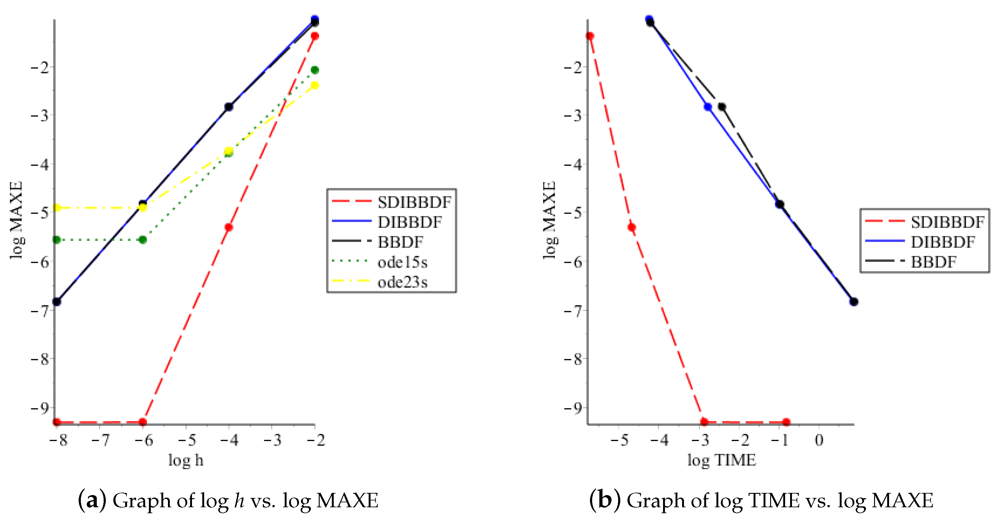
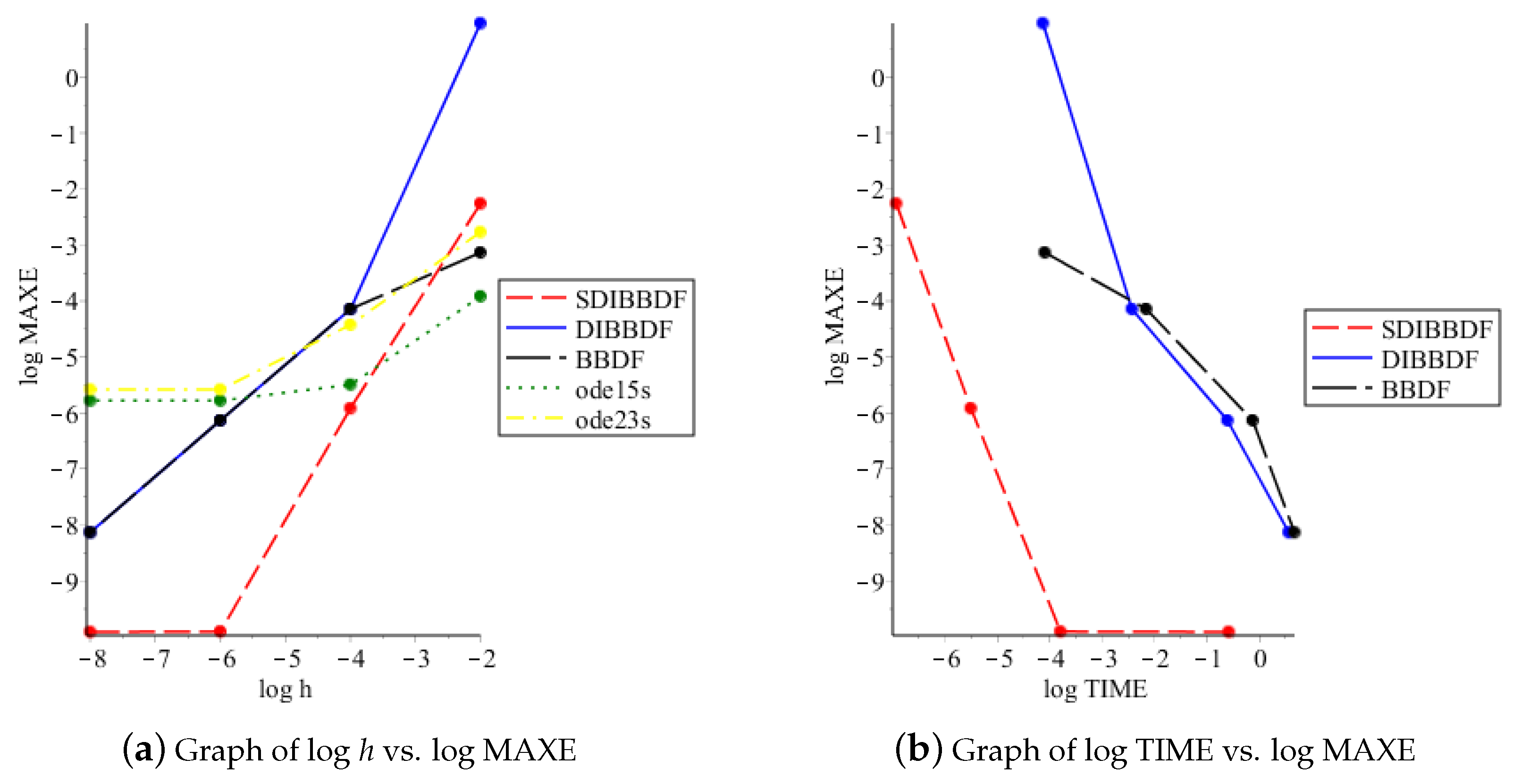
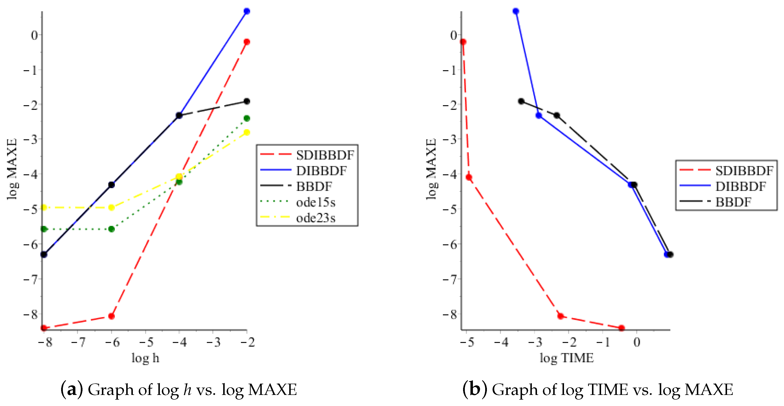
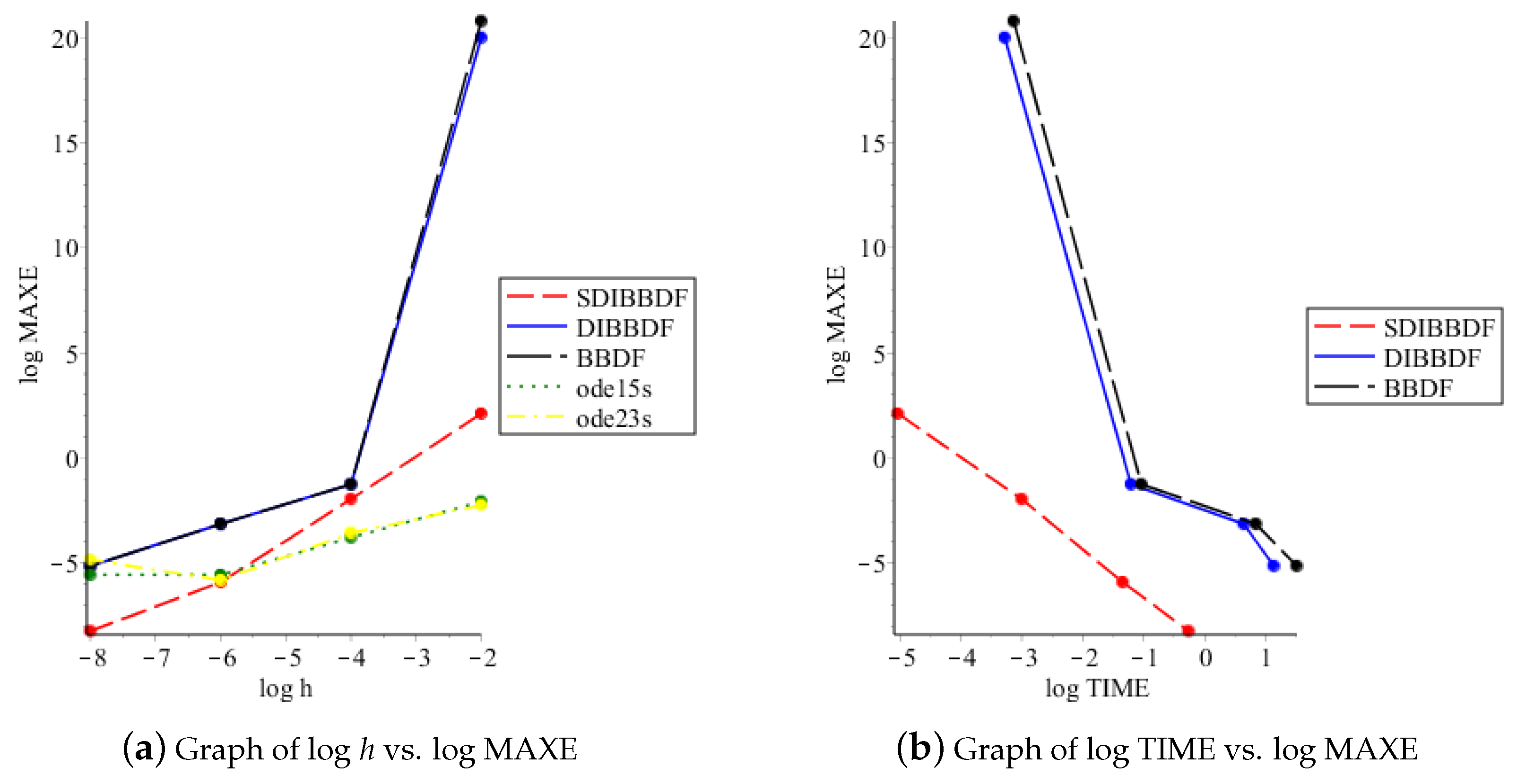
	ode23s	$2.07004\times {10}^{-1}$	-

represent the numerical approximations of SDIBBDF, DIBBDF, BBDF, ode15s and ode23s for stiff ODEs with various step size. The results are illustrated in the form of efficiency curves as shown in Figure 5, Figure 6, Figure 7, Figure 8 and Figure 9. Figure 5a, Figure 6a, Figure 7a, Figure 8a and Figure 9a indicate performance of the methods based on step sizes tested. Meanwhile, Figure 5b, Figure 6b, Figure 7b, Figure 8b and Figure 9b give visual representations on efficiency of the methods in terms of computational time to approximate solutions.

Matlab solvers, ode15s and ode23s, are chosen as comparing methods since both solvers are designed for solving stiff problems. Ode15s is a variable order solver based on the numerical differentiation formulas. For certain occasions, it uses the BDFs method. On the other hand, ode23s is a one-step solver based on a modified Rosenbrock formula of order 2. Since results for SDIBBDF, DIBBDF and FIBBDF methods are computed by using C++ programming languages, the TIME of those methods cannot be compared with the one from Matlab.

From the results, one can observed that Matlab solvers, ode15s and ode23s, managed to obtain smaller MAXE than the SDIBBDF method when computing solutions for $h={10}^{-2}$ for every test problems. Numerical results in Table 3 show that SDIBBDF method produced slightly bigger MAXE than the fully implicit method when $h={10}^{-2}$. This is due to the step size restriction as discussed earlier in Section 2.3. Since test problem 2 has $\lambda =-100$ hence, it requires $h<0.006240609349$.

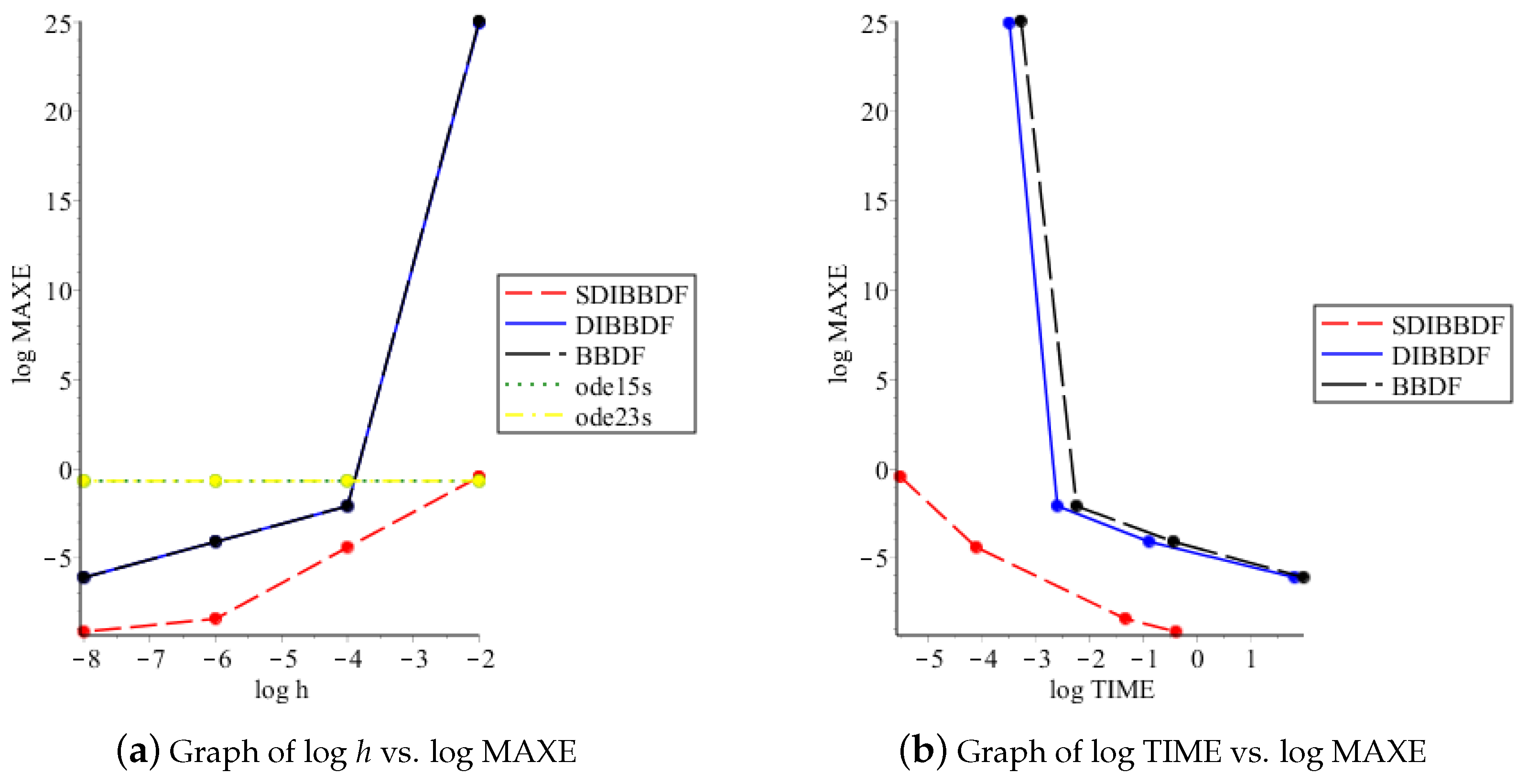
Not only that, but step size restriction is also experienced when $h={10}^{-2}$ is used to solve test problem 3 with $\lambda =-100$ and $-1$. Notice that the SDIBBDF, DIBBDF and BBDF method produced bigger MAXE for test problem 4 and 5 than the other test problems for stepsize $h=0.01$. The errors obtained by both test problems are affected by the nature of the system where test problem 4 involved a highly stiff ODEs with $\lambda =-1000$ and $-1$ while test problem 5 consists of complex eigenvalues, $\lambda =-40-40i,-40+40i$ and $-2$.

On the contrary, efficiency of the SDIBBDF method is proven when smaller stepsizes are used. It is capable of outperforming the other comparing methods for $h={10}^{-4}$, $h={10}^{-6}$ and $h={10}^{-8}$ for each problems of stiff ODEs tested.

As for TIME, the proposed method is capable of executing solutions faster than the fully and diagonally implicit methods for each test problem. This is motivated by the implementation of singly diagonally implicit properties that had proved to improve efficiency of the method. Figure 5b, Figure 6b, Figure 7b, Figure 8b and Figure 9b show that smaller step sizes require longer computational time due to larger number of steps involved.

4. Conclusions

The 2-point SDIBBDF method of order 2 for solving stiff ODEs is successfully derived by implementing the SDIRK properties of one-step method to the multistep block method. Stability analysis of the proposed method shows that it is zero-stable and with the A-stable characteristics which makes it fit for solving stiff problems.

Based on Section 2.3, we analysed the relation between step size and eigenvalue of stiff ODEs which gives effect on the MAXE produced. Hence, we will be able to set the best step size to used for solving stiff ODEs based on its eigenvalues in order to ensure good performance of SDIBBDF method to approximate solutions of the problems.

From numerical results, it is proved that the SDIBDDF method produced better accuracy for smaller stepsizes than the other comparing methods, and capable to execute solutions faster than the DIBBDF and fully implicit BBDF method. Effects of the step size restriction are also shown on the numerical results and analysed further.

Therefore, we can conclude that the SDIBBDF method can be used as an alternative solver for solving stiff ODEs.

References

1. Lambert, J.D. Computational Methods in Ordinary Differential Equations; John Wiley & Sons Ltd.: Great Britain, UK, 1973; ISBN 0-471-51194-3. [Google Scholar]
2. Johnson, A.I.; Barney, J.R. Numerical Methods for Differential System: Recent Developments in Algorithms, Software and Applications, 1st ed.; Lapidus, L., Schiesser, W., Eds.; Academic Press Inc.: New York, NY, USA, 1976; ISBN 9781483269856. [Google Scholar]
3. Milne, W.E. Numerical Solution of Differential Equations; John Wiley & Sons: New York, NY, USA, 1953. [Google Scholar]
4. Chu, M.T.; Hamilton, H. Parallel solution of ODE’s by multi-block methods. SIAM J. Sci. Stat. Comput. 1987, 8, 342–353. [Google Scholar] [CrossRef]
5. Rosser, J.B. A Runge-Kutta for all seasons. SIAM Rev. 1967, 9, 417–452. [Google Scholar] [CrossRef]
6. Shampine, L.F.; Watts, H.A. Block implicit one-step method. Math. Comput. 1969, 23, 731–740. [Google Scholar] [CrossRef]
7. Omar, Z.B.; Suleiman, M.B. Solving Higher Order ODEs using Parallel 2-Point Explicit Block Method. Matematika 2005, 21, 15–23. [Google Scholar]
8. Majid, Z.A.; Suleiman, M.B. Implementation of Parallel Three-Point Block Codes for Solving Large Systems of ODEs. Int. J. Comp. Math. 2010, 87, 1415–1429. [Google Scholar] [CrossRef]
9. Ibrahim, Z.B.; Suleiman, M.; Othman, K.I. Fixed coefficients block backward differentiation formulas for the numerical solution of stiff ordinary differential equations. Eur. J. Sci. Res. 2008, 21, 508–520. [Google Scholar]
10. Suleiman, M.B. Generalized Multistep Adams and Backward Differentiation Methods for the Solution of Stiff and Non-stiff Ordinary Differential Equations. Ph.D. Thesis, Universiti Putra Malaysia, Selangor, Malaysia, 1979. [Google Scholar]
11. Zawawi, I.S.M.; Ibrahim, Z.B.; Ismail, F.; Majid, Z.A. Diagonally implicit block backward differentiation formulas for solving ordinary differential equations. Int. J. Math. Math. Sci. 2012, 2012, 767328. [Google Scholar] [CrossRef]
12. Majid, Z.A.; Suleiman, M.B. Performance of 4-point diagonally implicit block method for solving ordinary differential equations. Matematika 2006, 22, 137–146. [Google Scholar]
13. Norsett, S.P. Semi-Explicit Runge-Kutta Methods; Report Mathematics and Computation No. 6/74; Dept. of Mathematics, University of Trondheim: Trondheim, Norway, 1974. [Google Scholar]
14. Alexander, R. Diagonally implicit Runge-Kutta methods for stiff O.D.E.’s. SIAM J. Numer. Anal. 1977, 14, 1006–1021. [Google Scholar] [CrossRef]
15. Burrage, K. A special family of Runge-Kutta methods for solving stiff differential equations. BIT 1978, 18, 22–41. [Google Scholar] [CrossRef]
16. Al-Rabeh, A.H. A variable parameter embedded DIRK algorithm for the numerical integration of stiff systems of ODEs. Comp. Math. Appl. 1987, 13, 373–379. [Google Scholar] [CrossRef]
17. D’Ambrosio, R.; Paternoster, B. Exponentially fitted singly diagonally implicit Runge-Kutta methods. J. Comput. Appl. Math. 2014, 263, 277–287. [Google Scholar] [CrossRef]
18. Kvaerno, K. Singly diagonally implicit Runge-Kutta methods with an explicit first stage. BIT Numer. Math. 2004, 44, 489–502. [Google Scholar] [CrossRef]
19. Senu, N.; Suleiman, M.; Othman, F.I. A singly diagonally implicit Runge-Kutta-Nystrom method for solving oscillatory problems. IAENG Int. J. Appl. Math. 2011, 41, 155–161. [Google Scholar]
20. Stal, J. Implementation of Singly Diagonally Implicit Runge-Kutta Methods with Constant Step Sizes. Bachelor’s Thesis, Lund University, Lund, Sweden, 2015. [Google Scholar]
21. Ababneh, O.Y.; Ahmad, R.; Ismail, E.S. Design of new diagonally implicit Runge-Kutta methods for stiff problems. Appl. Math. Sci. 2009, 3, 2241–2253. [Google Scholar]
22. Dahlquist, G.G. A special stability problem for linear multistep methods. BIT Numer. Math. 1963, 3, 27–43. [Google Scholar] [CrossRef]
23. Zawawi, I.S.M. Diagonally Implicit Block Backward Differentiation Formulas for Solving Fuzzy Differential Equations. Master’s Thesis, Universiti Putra Malaysia, Selangor, Malaysia, 2014. [Google Scholar]
24. Ibrahim, Z.B. Block Method for Multistep Formulas for Solving Ordinary Differential Equations. Ph.D. Thesis, Universiti Putra Malaysia, Selangor, Malaysia, 2006. [Google Scholar]
25. Burden, R.L.; Faires, J.D. Numerical Analysis, 7th ed.; Brooks/Cole: Boston, MA, USA, 2001; Volume 1, ISBN 9780534382162. [Google Scholar]
26. Gear, C.W. Numerical intial value problems in ordinary differential equations. Commmun. ACM 1971, 14, 185–190. [Google Scholar] [CrossRef]
Figure 1. 2-point SDIBBDF method of constant step size.
Mathematics 07 00211 g001
Figure 2. MAPLE codes to construct stability graph of 2-point SDIBBDF method.
Mathematics 07 00211 g002
Figure 3. Stability graph of 2-point SDIBBDF method.
Mathematics 07 00211 g003
Figure 4. Comparison of stability graph between SDIBBDF, BBDF and DIBBDF method.
Mathematics 07 00211 g004
Figure 5. Efficiency curves for test problem 1.
Mathematics 07 00211 g005
Figure 6. Efficiency curves for test problem 2.
Mathematics 07 00211 g006
Figure 7. Efficiency curves for test problem 3.
Mathematics 07 00211 g007
Figure 8. Efficiency curves for test problem 4.
Mathematics 07 00211 g008
Figure 9. Efficiency curves for test problem 5.
Mathematics 07 00211 g009