Cumulative Measure of Inaccuracy and Mutual Information in k-th Lower Record Values

Abstract

In this paper, we discuss the cumulative measure of inaccuracy in k-lower record values and study characterization results of dynamic cumulative inaccuracy. We also present some properties of the proposed measures, and the empirical cumulative measure of inaccuracy in k-lower record values. We prove a central limit theorem for the empirical cumulative measure of inaccuracy under exponentially distributed populations. Finally, we analyze the mutual information for measuring the degree of dependency between lower record values, and we show that it is distribution-free.

1. Introduction and Background

The Information Theory provides various concepts of broad use in Probability and Statistics which are finalized to measure the information content of stochastic models. Apart from the classical differential entropy, which constitutes a useful tool for the analysis of absolutely continuous random variables, some information measures based on cumulative notions have been attracting an increasing amount of attention in the recent literature. Among such measures, in this paper we focus on the cumulative (past) inaccuracy of bivariate random lifetimes, which is a suitable extension of the cumulative entropy. We also deal with the mutual information, which is strictly related to the Shannon entropy, and is one of the most commonly adopted notions for bivariate random variables. Indeed, the mutual information is a measure of the mutual dependence of two random variables, and can be evaluated by means of the joint (and marginal) distributions.

We recall some recent papers dealing with stochastic models and information measures of interest in the reliability theory. Navarro et al. [1] presented some stochastic ordering and properties of aging classes of dynamic cumulative residual entropy, where Psarrakos and Navarro [2] generalized the concept of cumulative residual entropy by relating this concept to the mean time between record values, and also considered the dynamic version of this new measure. Moreover, Tahmasebi and Eskandarzadeh [3] proposed a new extension of the cumulative entropy based on k-th lower record values. Sordo and Psarrakos [4] provided comparison results for the cumulative residual entropy of systems and their dynamic versions.

Motivated by some of the articles mentioned above, in this paper we aim to investigate some applications of the previously mentioned information measures to the k-lower record values. Record values are widely studied in the literature as a suitable tool to convey essential information in stochastic models. More recently, they have also been attracting attention in applied contexts related to high-dimensional data, where it is computationally more convenient to determine the rank rather than the specific values of the observations under investigation.

More specifically, within the scope of this paper, we propose to study the cumulative measure of inaccuracy in k-lower record values and the parent random variable of a random sample. The context of dynamic observations will be also considered by analyzing the dynamic cumulative inaccuracy and related characterization results. We present some properties of the proposed measures, as well as the empirical cumulative measure of inaccuracy in k-lower record values. Moreover, the investigation focuses also on the mutual information measure, finalized to measure the degree of dependency between lower record values.

In the remaining part of this section, we recall the relevant notions that will be used in the following, and provide the plan of the paper. Specifically, we discuss the basic definitions and properties of the information measures mentioned above, i.e., the cumulative inaccuracy and the mutual information. Then, we mention the essential results on the lower record values and recall certain useful stochastic orders. We shall look into nonnegative random variables, with the case of truncated support being treatable in a similar way.

Throughout the paper, “log” means natural logarithm, prime denotes derivative, and the terms “increasing” and “decreasing” are used in a non-strict sense. Finally, as is customary, we assume that $0log0$ is vanishing.

1.1. Notions of Information Theory

Consider an absolutely continuous random vector $(X,Y)$ having nonnegative components. We denote by $f(x,y)$ the joint probability density function (PDF) by $f(x)$ and $g(x)$, the marginal PDFs, and by $F(x)$ and $G(x)$, the cumulative distribution functions (CDFs) of X and Y, respectively.

Bearing in mind the applications in the reliability theory, we assume that X and Y denote random lifetimes of suitable systems having support $(0,\infty )$. Let

$$H(X)=-\mathbb{E}[log(f(X))]=-{\int }_0^{\infty }f(x)log(f(x))dx$$

(1)

be the (Shannon) differential entropy of X. $H(Y)$ is defined similarly, and the bivariate entropy of $(X,Y)$ is given by $H(X,Y)=-\mathbb{E}[log(f(X,Y))]=-{\int }_0^{\infty }dx{\int }_0^{\infty }f(x,y)log(f(x,y))dy$. Moreover, the conditional entropy of Y given by X is expressed by:

$$H(Y|X)=-{\int }_0^{\infty }dx{\int }_0^{\infty }f(x,y)log\left({\displaystyle \frac{f(x,y)}{f(x)}}\right)dy,$$

(2)

whereas the mutual information of $(X,Y)$ is defined as:

$$M_{X,Y}={\int }_0^{\infty }dx{\int }_0^{\infty }f(x,y)log\left({\displaystyle \frac{f(x,y)}{f(x)g(y)}}\right)dy.$$

(3)

We recall that $M_{X,Y}$ is a measure of dependence between X and Y, with $M_{X,Y}=0$ if, and only if X and Y are independent. Furthermore, $M_{X,Y}$ is largely adopted to assess the information content in a variety of applied fields, such as signal processing and pattern recognition. Due to (3), the mutual information can be expressed in terms of suitable entropies as follows (see, for example, Ebrahimi et al. [5]):

$$M_{X,Y}=H(X)+H(Y)-H(X,Y)=H(Y)-H(Y|X).$$

(4)

See also Ebrahimi et al. [6] and Ahmadi et al. [7] for various results of interest in the reliability theory involving dynamic measures for multivariate distributions based on the mutual information.

Among the notions involving cumulative versions of information measures, we now recall the cumulative (past) inaccuracy of $(X,Y)$, given by:

$$I(X,Y)=-{\int }_0^{\infty }F(x)log(G(x))dx.$$

(5)

As specified in Section 1 of Kundu et al. [8], the measure given in (5) can be viewed as the cumulative analogue of the Kerridge inaccuracy measure of X and Y, which is expressed as $-{\int }_0^{\infty }f(x)log(g(x))dx$ (cf. Kerridge [9]). The relevant difference is that Equation (5) involves the CDFs instead of the PDFs. In many real situations, it is more convenient to deal with distribution functions which carry information about the fact that an event occurs prior or after the current time. Moreover, the measure given in (5) provides information content when using $G(x)$, the CDF asserted by the experimenter due to missing or incorrect information in experiments, instead of the true distribution $F(x)$. Clearly, if F and G are identical, then $I(X,Y)$ identifies with the cumulative entropy studied by Di Crescenzo and Longobardi [10] and by Navarro et al. [1]. See Section 5 of Kumar and Taneja [11] for various results involving (5) and the related dynamic version, i.e., the dynamic cumulative past inaccuracy measure. We finally recall that the cumulative inaccuracy (5) and the cumulative entropy are also involved in the definition of other information measures of interest (see, for instance, Park et al. [12], and Di Crescenzo and Longobardi [13] for the cumulative Kullback-Leibler information).

1.2. Lower Record Values

Record values are often studied in various fields due to their relevance in specific applications. If statistical observations are difficult to obtain, or when experimental observations are destroyed and access to them is not available, then the researchers are forced to make inference about the distribution of the observations of used record amounts. Suppose, for example, that it is required to estimate the water level of a river solely based on the available records of previous flooding. Similarly, consider variables such as record rainfall, record temperature, wind speed record, and other quantities of interest in meteorology. In such cases, the analysis of statistical observations, if performed by resorting to lower or upper record values.

Let us now recall some basic notions about lower record values that will be used in this paper. Let X be an absolutely continuous nonnegative random variable with CDF $F(x)$ and PDF $f(x)$, and let $\{X_n,n\ge 1\}$ be a sequence of independent random variables, distributed identically as X. An observation $X_j$, $j\ge 1$, will be called a lower record value if its value is less than the values of all previous observations. Thus, $X_j$ is a lower record value if $X_j<X_i$ for every $i<j$. For a fixed positive integer k, similarly to Dziubdziela and Kopociński [14], we define the sequence $\{T_{n(k)},n\ge 1\}$ of k-th lower record times for the sequence $\{X_n,n\ge 1\}$ as follows:

$$T_{1(k)}=1,T_{n+1(k)}=min\left\{j>T_{n(k)}:X_{k:T_{n(k)}+k-1}>X_{k:k+j-1}\right\},$$

(6)

where $X_{j:m}$ denotes the j-th order statistic in a sample of size m (see also Malinowska and Szynal [15]). Then,

$$L_{n(k)}:=X_{k:T_{n(k)}+k-1},$$

is called a sequence of k-th lower record values of $\{X_n,n\ge 1\}$. Since the ordinary record values are contained in the k-records, the results for usual records can be obtained as a special case by setting $k=1$. The PDF of $L_{n(k)}$, for $n\ge 1$ and $k\ge 1$, is given by:

$$f_{n(k)}(x)={\displaystyle \frac{k^n}{(n-1)!}}{\left[F(x)\right]}^{k-1}{\left[\tilde{\Lambda }(x)\right]}^{n-1}f(x),$$

(7)

and the joint PDF of $(L_{m(k)},L_{n(k)})$, for $1\le m<n$, $k\ge 1$, is:

$$\begin{array}{cc}\hfill f_{m(k),n(k)}(x,y)& ={\displaystyle \frac{k^n}{(m-1)!(n-m-1)!}}{[\tilde{\Lambda }(y)-\tilde{\Lambda }(x)]}^{n-m-1}\hfill \\ & \times {\left[\tilde{\Lambda }(x)\right]}^{m-1}h(x){\left[F(y)\right]}^{k-1}f(y),x>y,\hfill \end{array}$$

(8)

where

$$\tilde{\Lambda }(x)=-logF(x)\mathrm{and}h(x)=-{\tilde{\Lambda }}^{\prime }(x)={\displaystyle \frac{f(x)}{F(x)}},x>0,$$

(9)

are the cumulative reversed hazard rate and the reversed hazard rate of X, respectively. Hence, the conditional PDF of $L_{n(k)}$ given $L_{m(k)}$, $1\le m<n$, is given by:

$$f_{n|m}(y|x)={\displaystyle \frac{k^n{[\tilde{\Lambda }(y)-\tilde{\Lambda }(x)]}^{n-m-1}f(y){\left[F(y)\right]}^{k-1}}{k^m(n-m-1)!{\left[F(x)\right]}^k}},x>y.$$

(10)

By using the well-known relation

$${\int }_z^{\infty }{\displaystyle \frac{{\lambda }^n}{(n-1)!}}{x}^{n-1}{e}^{-\lambda x}dx={\displaystyle \sum _{i=0}^{n-1}}{\displaystyle \frac{{\left[\lambda z\right]}^i}{i!}}{e}^{-\lambda z},$$

we see that the CDF corresponding to Equation (7) can be obtained as:

$$\begin{array}{cc}{F}_{n(k)}(x)\hfill & ={\int }_0^x{\displaystyle \frac{k^n}{(n-1)!}}{\left[F(y)\right]}^{k-1}{\left[\tilde{\Lambda }(y)\right]}^{n-1}f(y)dy\hfill \\ & ={\left[F(x)\right]}^k{\displaystyle {\sum }_{i=0}^{n-1}}{\displaystyle \frac{{\left[k\tilde{\Lambda }(x)\right]}^i}{i!}}.\hfill \end{array}$$

(11)

We note that the sequence of k-th upper record times is denoted as $\{U_{n(k)},n\ge 1\}$. It is defined similarly to $T_{n(k)}$ by reverting the last inequality in (6) (see, for instance, Dziubdziela and Kopociński [14] or Tahmasebi et al. [16]). Record values apply in problems such as industrial stress testing, meteorological analysis, hydrology, sport, and economics. In reliability theory, record values are used to study things such as technical systems which are subject to shocks, e.g., peaks of voltages. For more details about records and their applications, one may refer to Arnold et al. [17]. Several authors investigated measures of inaccuracy for ordered random variables. Thapliyal and Taneja [18] proposed the measure of inaccuracy between the i-th order statistic and the parent random variable. Moreover, Thapliyal and Taneja [19] developed measures of dynamic cumulative residual and past inaccuracy. They studied characterization results of these dynamic measures under a proportional hazard model and proportional reversed hazard model. The same authors introduced the measure of residual inaccuracy of order statistics and proved a related characterization result (cf. Thapliyal and Taneja [20]). Equality of Rényi entropies of upper and lower k-records is also known to provide a characteristic property of symmetric distributions (see Fashandi and Ahmadi [21]). Furthermore, it is worth mentioning that the analysis of lower record values is related to the generalized cumulative entropy. For instance, its role in the study of a new measure of association based on the log-odds rate has recently been pinpointed by Asadi [22]. Finally, recent contributions on a measure of past entropy for nth upper k-record values can be found in Goel et al. [23].

1.3. Stochastic Orders and Related Notions

Aiming to use stochastic orders to perform suitable comparisons, here we recall some relevant definitions. Let X and Y be random variables, where X is said to be smaller than Y, according to the

-

usual stochastic ordering (denoted by $X{\le }_{st}Y$) if $\mathbb{P}(X\ge x)\le \mathbb{P}(Y\ge x)$ for all $x\in \mathbb{R}$; it is known that $X{\le }_{st}Y\iff \mathbb{E}(\varphi (X))\le \mathbb{E}(\varphi (Y))$ for all increasing functions $\varphi$;

-

likelihood ratio ordering (denoted by $X{\le }_{lr}Y$) if ${\displaystyle \frac{g(x)}{f(x)}}$ is increasing in x;

-

decreasing convex order, denoted by $X{\le }_{dcx}Y$, if $\mathbb{E}(\varphi (X))\le \mathbb{E}(\varphi (Y))$ for all decreasing convex functions $\varphi$, such that the expectations exist.

Moreover, we say that X has a decreasing reversed hazard rate (DRHR) if $h(x)={\displaystyle \frac{f(x)}{F(x)}}$ is decreasing in x. For specific details on these notions, see, for instance, Shaked and Shanthikumar [24], and for applications of the decreasing convex order, see Ma [25].

1.4. Plan of the Paper

In this investigation, we propose the cumulative measure of inaccuracy and study characterization results of a dynamic cumulative inaccuracy measure. Also, we study the degree of dependency among the sequence of k-th lower record values through the mutual information of record values.

The paper is organized as follows: In Section 2, we consider a measure of inaccuracy associated with $L_{n(k)}$ and X. We provide some results and properties of such a measure, including an application to the proportional reversed hazards model. In Section 3, we propose the dynamic version of inaccuracy associated with $L_{n(k)}$ and X, and provide a characterization result. In Section 4, we study the problem of estimating the cumulative measure of inaccuracy by means of the empirical cumulative inaccuracy in k-lower record values. The rest of the section is devoted to a simple application to real data, with the discussion of some special cases, and a central limit theorem for the empirical cumulative measure of inaccuracy in the case of exponentially distributed random samples. Finally, in Section 5 we investigate the mutual information between sequences of lower record values, aiming to measure their degree of dependency. Specifically, we show that this measure is distribution-free and can be computed by using the distribution of the k-th lower record values of the sequence from the uniform distribution.

2. Cumulative Measure of Inaccuracy

Let us now consider the cumulative measure of inaccuracy between $L_{n(k)}$ and the parent non-negative random variable, say X. Recalling (5) and (11), we have:

$$\begin{array}{cc}I(L_{n(k)},X)\hfill & =-{\int }_0^{\infty }{F}_{n(k)}(x)log\left(F(x)\right)dx\hfill \\ & ={\displaystyle {\sum }_{i=0}^{n-1}}{\displaystyle \frac{k^i}{i!}}{\int }_0^{\infty }{\left[F(x)\right]}^k{\left[\tilde{\Lambda }(x)\right]}^{i+1}dx,\hfill \end{array}$$

(12)

with $\tilde{\Lambda }(x)$ given in (9). According to the comments given in Section 1.1, $I(L_{n(k)},X)$ can be used to gain information concerning an experiment for which the distribution of the k-lower record values is compared with the parent distribution. Noting that, due to (7), $L_{i+2(k)}$ being a random variable with density function

$$f_{i+2(k)}(x)={\displaystyle \frac{k^{i+2}}{(i+1)!}}{\left[F(x)\right]}^{k-1}{\left[\tilde{\Lambda }(x)\right]}^{i+1}f(x),$$

and recalling that $h(x)$ is the reversed hazard rate of X (see (9)), from (12) we obtain:

$$\begin{array}{cc}I(L_{n(k)},X)\hfill & ={\displaystyle {\sum }_{i=0}^{n-1}}{\displaystyle \frac{i+1}{k^2}}{\int }_0^{\infty }{\displaystyle \frac{k^{i+2}}{(i+1)!}}{\left[F(x)\right]}^k{\left[\tilde{\Lambda }(x)\right]}^{i+1}dx\hfill \\ & ={\displaystyle {\sum }_{i=0}^{n-1}}{\displaystyle \frac{i+1}{k^2}}\mathbb{E}\left[{\displaystyle \frac{1}{h(L_{i+2(k)})}}\right].\hfill \end{array}$$

(13)

Remark 1.

Making use of the generalized cumulative entropy introduced in Definition 1.1 of Tahmasebi and Eskandarzadeh [3], given by:

$${\mathcal{CE}}_{i+1,k}(X)={\int }_0^{\infty }{\displaystyle \frac{k^{i+2}}{(i+1)!}}{\left[F(x)\right]}^k{\left[\tilde{\Lambda }(x)\right]}^{i+1}dx\equiv \mathbb{E}\left[{\displaystyle \frac{1}{h(L_{i+2(k)})}}\right],$$

(14)

from (13) one has that the cumulative measure of inaccuracy between $L_{n(k)}$ and X can be expressed: as a size-biased combination of generalized cumulative entropies through the following weighted sum with linearly increasing weights:

$$I(L_{n(k)},X)={\displaystyle \frac{1}{k^2}}{\displaystyle \sum _{i=1}^n}i{\mathcal{CE}}_{i,k}(X).$$

(15)

Furthermore, from (11) and (12) we obtain an alternative expression, that is:

$$I(L_{n(k)},X)={\displaystyle \sum _{i=0}^{n-1}}{\int }_0^{\infty }\tilde{\Lambda }(x)[F_{i+1(k)}(x)-F_{i(k)}(x)]dx.$$

In the following proposition we provide another form of $I(L_{n(k)},X)$.

Proposition 1.

Let X be a nonnegative random variable with cdf F; for the cumulative measure of inaccuracy between $L_{n(k)}$ and X, we have:

$$I(L_{n(k)},X)={\displaystyle \sum _{i=0}^{n-1}}{\displaystyle \frac{k^i}{i!}}{\int }_0^{+\infty }h(z)\left\{{\int }_0^z{\left[F(x)\right]}^k{\left[\tilde{\Lambda }(x)\right]}^{i}dx\right\}dz.$$

(16)

Proof. 

By (12) and the relation $-logF(x)={\int }_x^{\infty }h(z)dz$, we have:

$$I(L_{n(k)},X)={\displaystyle \sum _{i=0}^{n-1}}{\displaystyle \frac{k^i}{i!}}{\int }_0^{+\infty }{\int }_x^{\infty }h(z){\left[F(x)\right]}^k{\left[\tilde{\Lambda }(x)\right]}^{i}dzdx.$$

By using Fubini’s theorem, we get:

$$I(L_{n(k)},X)={\displaystyle \sum _{i=0}^{n-1}}{\displaystyle \frac{k^i}{i!}}{\int }_0^{+\infty }{\int }_0^{z}h(z){\left[F(x)\right]}^k{\left[\tilde{\Lambda }(x)\right]}^{i}dxdz,$$

and the result thus follows. □

Hereafter, we present some examples and properties of $I(L_{n(k)},X)$.

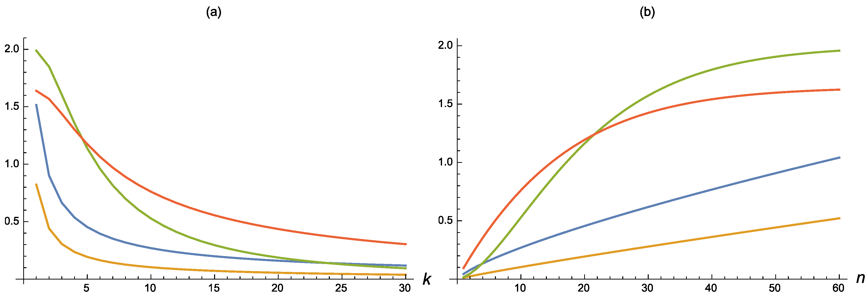
Example 1.

(i) 

If X is uniformly distributed in $[0,\theta ]$, then:

$$I(L_{n(k)},X)={\displaystyle \frac{\theta }{k^2}}{\displaystyle \sum _{i=0}^{n-1}}(i+1){\left({\displaystyle \frac{k}{k+1}}\right)}^{i+2}.$$

(ii) 

If X is exponentially distributed with mean ${\displaystyle \frac{1}{\lambda }}$, then:

$$I(L_{n(k)},X)={\displaystyle \frac{1}{\lambda }}{\displaystyle \sum _{i=0}^{n-1}}(i+1)k^i{\displaystyle \sum _{j=0}^{\infty }}{\left({\displaystyle \frac{1}{j+k+1}}\right)}^{i+2}.$$

(iii) 

If X has an inverse Weibull distribution with cdf $F(x)=exp\{-{({\displaystyle \frac{\alpha }{x}})}^{\beta }\}$, $x>0$, with $\alpha >0$ and $\beta >1$, then:

$$I(L_{n(k)},X)={\displaystyle \frac{\alpha }{\beta }}{k}^{{\displaystyle \frac{1}{\beta }}-1}{\displaystyle \sum _{i=0}^{n-1}}{\displaystyle \frac{1}{i!}}\Gamma \left({\displaystyle \frac{(i+1)\beta -1}{\beta }}\right).$$

For suitable choices of n and k, such inaccuracy measures are plotted in Figure 1, where the parameters are chosen so that the considered distributions have a unity mean, i.e., (i) $\theta =2$, (ii) $\lambda =1$, and (iii) $\alpha =1/\Gamma (1-{\beta }^{-1})$, recalling that the mean of an inverse Weibull distribution is $\mathbb{E}(X)=\alpha \Gamma (1-{\beta }^{-1})$ (see de Gusmão et al. [26]). In all cases, $I(L_{n(k)},X)$ is decreasing in k and increasing in n.

Let us now discuss the effect of identical linear transformations on $I(L_{n(k)},X)$.

Proposition 2.

Let $a>0$ and $b\ge 0$; for $n\in \mathbb{N}$, it holds that:

$$I(a{L}_{n(k)}+b,aX+b)=aI(L_{n(k)},X).$$

(17)

Proof. 

From (15), we have:

$$I(a{L}_{n(k)}+b,aX+b)={\displaystyle \frac{1}{k^2}}{\displaystyle \sum _{i=1}^n}i{\mathcal{CE}}_{i,k}(aX+b).$$

Recalling (14), it is not hard to see that: ${\mathcal{CE}}_{i,k}(aX+b)=a{\mathcal{CE}}_{i,k}(X)$, so that the proof immediately follows. □

Remark 2.

Let X be a symmetric random variable with respect to the finite mean $\mu =\mathbb{E}(X)$, i.e., $F(x+\mu )=1-F(\mu -x)$ for all $x\in \mathbb{R}$. Then the following relation holds:

$$I(L_{n(k)},X)=\overline{I}(R_{n(k)},X):=-{\int }_0^{\infty }{\overline{F}}_{n(k)}(x)log\left(\overline{F}(x)\right)dx,$$

where, similarly to (12), the latter term defines the cumulative residual measure of inaccuracy between the k-th upper record value and X. Here, as usual, $\overline{F}(x)=1-F(x)$ denotes the survival function of X, and ${\overline{F}}_{n(k)}(x)$ denotes the survival function of the k-th upper record value $R_{n(k)}$.

Hereafter, we obtain an upper bound for $I(L_{n(k)},X)$.

Proposition 3.

Let X be an absolutely continuous non-negative random variable with a cumulative reversed hazard rate $\tilde{\Lambda }(x)$, such that the following function is finite:

$$h_{i+1}^{\star }(t)={\int }_t^{\infty }{\left[\tilde{\Lambda }(x)\right]}^{i+1}dx,t>0.$$

(18)

Then, for $n\in \mathbb{N}$ we have:

$$I(L_{n(k)},X)\le {\displaystyle \sum _{i=0}^{n-1}}{\displaystyle \frac{k^i}{i!}}\mathbb{E}\left[h_{i+1}^{\star }(X)\right].$$

Proof. 

By (12), from ${\left[F(x)\right]}^k\le F(x)]$ and Fubini’s theorem, we obtain:

$$\begin{array}{cc}\hfill I(L_{n(k)},X)& \le {\displaystyle \sum _{i=0}^{n-1}}{\displaystyle \frac{k^i}{i!}}{\int }_0^{\infty }{\left[\tilde{\Lambda }(x)\right]}^{i+1}{\int }_0^{x}f(t)dtdx\hfill \\ & ={\displaystyle \sum _{i=0}^{n-1}}{\displaystyle \frac{k^i}{i!}}{\int }_0^{\infty }f(t){\int }_t^{\infty }{\left[\tilde{\Lambda }(x)\right]}^{i+1}dxdt\hfill \\ & ={\displaystyle \sum _{i=0}^{n-1}}{\displaystyle \frac{k^i}{i!}}\mathbb{E}\left[h_{i+1}^{*}(X)\right],\hfill \end{array}$$

thus completing the proof. □

Now we can prove a property of the considered inaccuracy measure by means of stochastic orderings. For that, we use the notions recalled in Section 1.3.

Theorem 1.

Suppose that the non-negative random variable X is DRHR. Then, for $n\in \mathbb{N}$, one has:

$$I(L_{n+1(k)},X)-I(L_{n(k)},X)\le {\displaystyle \frac{1}{k^2}}{\displaystyle \sum _{m=1}^{n+1}}\mathbb{E}\left[{\displaystyle \frac{1}{h(L_{m(k)})}}\right].$$

(19)

Proof. 

Recalling that $f_{n(k)}(x)$ is the PDF of $L_{n(k)}$, provided in Equation (7), then the ratio ${\displaystyle \frac{f_{n(k)}(x)}{f_{n+1(k)}(x)}}={\displaystyle \frac{-n}{klogF(x)}}$ is increasing in x. Therefore, $L_{n+1(k)}{\le }_{lr}{L}_{n(k)}$, and this implies that $L_{n+1(k)}{\le }_{st}{L}_{n(k)}$, i.e., $\mathbb{E}\left[\varphi (L_{n+1(k)})\right]\le \mathbb{E}\left[\varphi (L_{n(k)})\right]$ for all increasing functions $\varphi$ such that these expectations exist. (For more details, see Shaked and Shanthikumar [24]). Thus, since X is DRHR and $h(x)$ is its reversed hazard rate, then ${\displaystyle \frac{1}{h(x)}}$ is increasing in x. As a consequence, from (13) we have:

$$\begin{array}{cc}\hfill I(L_{n+1(k)},X)& ={\displaystyle \sum _{i=0}^n}{\displaystyle \frac{i+1}{k^2}}\mathbb{E}\left[{\displaystyle \frac{1}{h(L_{i+2(k)})}}\right]\hfill \\ & \le {\displaystyle \sum _{i=0}^n}{\displaystyle \frac{i+1}{k^2}}\mathbb{E}\left[{\displaystyle \frac{1}{h(L_{i+1(k)})}}\right]\hfill \\ & ={\displaystyle \sum _{j=-1}^{n-1}}{\displaystyle \frac{j+2}{k^2}}\mathbb{E}\left[{\displaystyle \frac{1}{h(L_{j+2(k)})}}\right]\hfill \\ & ={\displaystyle \sum _{j=0}^{n-1}}{\displaystyle \frac{j+2}{k^2}}\mathbb{E}\left[{\displaystyle \frac{1}{h(L_{j+2(k)})}}\right]+{\displaystyle \frac{1}{k^2}}\mathbb{E}\left[{\displaystyle \frac{1}{h(L_{1(k)})}}\right]\hfill \\ & =I(L_{n(k)},X)+{\displaystyle \frac{1}{k^2}}{\displaystyle \sum _{i=1}^{n+1}}\mathbb{E}\left[{\displaystyle \frac{1}{h(L_{i(k)})}}\right],\hfill \end{array}$$

where $I(L_{n(k)},X)$ is expressed in (13). The proof is thus completed. □

Theorem 2.

Let X and Y be two non-negative random variables, such that $X{\le }_{dcx}Y$; then we have:

$$I(L_{n(k)},X)\le I(L_{n(k)}^G,Y):=-{\int }_0^{\infty }{G}_{n(k)}(y)log(G(y))dy.$$

Here, similarly to (6), $L_{n(k)}^G$ denotes the k-th lower record times for the sequence $\{Y_n,n\ge 1\}$ with distribution function $G_{n(k)}(y)$, and $G(y)$ is the distribution function of Y.

Proof. 

Due to (18), $h_{j+1}^{\star }(x)$ is a decreasing convex function in x. The proof then immediately follows from Proposition 3. □

Let us now investigate the cumulative measure of inaccuracy within the proportional reversed hazards model (PRHM). We recall that two random variables X and $X_{\theta }^{*}$ satisfy the PRHM if their distribution functions are related by the following identity, for $\theta >0$:

$$F_{\theta }^{*}(x)={\left[F(x)\right]}^{\theta },x\in \mathbb{R}.$$

(20)

For some properties of such a model associated with aging notions and the reversed relevation transform, see Gupta and Gupta [27] and Di Crescenzo and Toomaj [28], respectively.

In this case, we assume that X and $X_{\theta }^{*}$ are non-negative, absolutely continuous random variables. Due to Equation (20) and making use of (5) and (11), and noting that ${\tilde{\Lambda }}_{\theta }^{*}(x)=\theta \tilde{\Lambda }(x)$, we obtain the cumulative measure of inaccuracy between $L_{n(k)}^{*}$ and $X_{\theta }^{*}$ as follows, for $\theta >0$:

$$\begin{array}{cc}I(L_{n(k)}^{*},X_{\theta }^{*})\hfill & =-{\int }_0^{+\infty }{F}_{n(k)}^{*}(x)log\left(F_{\theta }^{*}(x)\right)dx\hfill \\ & ={\displaystyle {\sum }_{i=0}^{n-1}}{k}^i{\theta }^{i+1}{\int }_0^{+\infty }{\displaystyle \frac{{\left[\tilde{\Lambda }(x)\right]}^{i+1}}{i!}}{\left[F(x)\right]}^{k\theta }dx,\hfill \end{array}$$

(21)

with $\tilde{\Lambda }(x)$ expressed in (9). Moreover, if $\theta$ is a positive integer, then the last expression can be rewritten in terms of the generalized cumulative entropy (14) as follows:

$$I(L_{n(k)}^{*},X_{\theta }^{*})={\displaystyle \frac{1}{k^2\theta }}{\displaystyle \sum _{i=0}^{n-1}}(i+1){\mathcal{CE}}_{i+1,k\theta }(X).$$

We recall that in this case, i.e., when $\theta \in \mathbb{N}$, the PRHM expresses that $X_{\theta }^{*}$ is distributed as the first-order statistics of a random sample having size $\theta$ and taken from the distribution of X.

Let us now obtain suitable bounds under the PRHM.

Proposition 4.

Let X and $X_{\theta }^{*}$ be non-negative, absolutely continuous random variables satisfying the PRHM as specified in (20), with $\theta >0$. If $\theta \ge (\le )1$, then for any $n\in \mathbb{N}$ we have:

$$I(L_{n(k)}^{*},X_{\theta }^{*})\le (\ge ){\displaystyle \frac{{\theta }^{i+1}}{k^2}}{\displaystyle \sum _{i=0}^{n-1}}(i+1){\mathcal{CE}}_{i+1,k}(X).$$

Proof. 

Clearly, for $\theta \ge (\le )1$ it is ${\left[F(x)\right]}^{k\theta }\le (\ge ){\left[F(x)\right]}^k$ for all $x\ge 0$, and then the thesis immediately follows from (14) and (21). □

We conclude this section with a remark on the cumulative measure of inaccuracy for bivariate first lower record values.

Remark 3.

Consider two identically distributed sequences of random variables $\{X_n,n\ge 1\}$ and $\{Y_m,m\ge 1\}$, and denote by $L_{n,X}=L_{n(1),X}$ and $L_{m,Y}=L_{m(1),Y}$ the corresponding first lower record times. Then, for $k=1$ and making use of (11) it is not hard to see that the cumulative measure of inaccuracy between $L_{n,X}$ and $L_{m,Y}$ is given by:

$$\begin{array}{cc}\hfill I(L_{n,X},L_{m,Y})& =-{\int }_0^{+\infty }{F}_n(x)log(F_m(x))\hfill \\ & ={\displaystyle \sum _{i=0}^{n-1}}(i+1)\mathbb{E}\left({\displaystyle \frac{1}{h(L_{i+1}(x))}}\right)-{\displaystyle \sum _{i=0}^{n-1}}{\int }_0^{+\infty }{\displaystyle \frac{F(x){\left[\tilde{\Lambda }(x)\right]}^i}{i!}}log\left({\displaystyle \sum _{i=0}^{m-1}}{\displaystyle \frac{{\left[\tilde{\Lambda }(x)\right]}^i}{i!}}\right),\hfill \end{array}$$

where $h(x)$ is the reversed hazard rate of the underlying distribution.

3. Dynamic Cumulative Measure of Inaccuracy

In this section, we study the dynamic version of the inaccuracy measure $I(L_{n(k)},X)$. Let X be the random lifetime of a brand new system that begins to work at time 0 and is observed only at deterministic inspection times. Clearly, if the system is found failed at time t, then the conditional distribution function of $\left[X\right|X\le t]$, known as the past lifetime, is given by ${\displaystyle \frac{F(x)}{F(t)}}$, $0\le x\le t$. In a sequence of i.i.d. failure times having the same distribution as X, if the information about the k-th lower failure times is available, then ${\displaystyle \frac{F_{n(k)}(x)}{F_{n(k)}(t)}}$ is the conditional probability that the k-th lower failure time is smaller that x, given that it is smaller than t, for $0\le x\le t$, where $F_{n(k)}(x)$ is the CDF given in (11). Hence, the dynamic cumulative measure of inaccuracy between $L_{n(k)}$ and X is expressed by the inaccuracy measure between the corresponding past lifetimes, i.e.,:

$$\begin{array}{cc}I(L_{n(k)},X;t)\hfill & =-{\int }_0^t{\displaystyle \frac{F_{n(k)}(x)}{F_{n(k)}(t)}}log\left({\displaystyle \frac{F(x)}{F(t)}}\right)dx\hfill \\ & ={\mu }_{n(k)}(t)log(F(t))-{\displaystyle \frac{1}{F_{n(k)}(t)}}{\int }_0^t{F}_{n(k)}(x)log(F(x))dx\hfill \\ & ={\mu }_{n(k)}(t)log(F(t))+{\displaystyle \frac{1}{F_{n(k)}(t)}}{\displaystyle {\sum }_{i=0}^{n-1}}{\int }_0^t{\displaystyle \frac{k^i}{i!}}{\left[F(x)\right]}^k{\left[\tilde{\Lambda }(x)\right]}^{i+1}dx,\hfill \end{array}$$

(22)

where

$${\mu }_{n(k)}(t)={\int }_0^t{\displaystyle \frac{F_{n(k)}(x)}{F_{n(k)}(t)}}dx$$

is the mean inactivity time of the random variable $[t-L_{n(k)}\mid L_{n(k)}<t]$. Clearly, recalling (12) and assuming that X is a bona fide random variable, from (22) we have ${lim}_{t\to \infty }I(L_{n(k)},X;t)=I(L_{n(k)},X)$. Moreover, if $F(t)>0$ for all $t>0$, since $logF(t)\le 0$, we immediately have:

$$I(L_{n(k)},X;t)\le {\displaystyle \frac{I(L_{n(k)},X)}{F_{n(k)}(t)}}.$$

We can now obtain a characterization result for $I(L_{n(k)},X;t)$.

Theorem 3.

Let X be a non-negative, absolutely continuous random variable with distribution function $F(x)$. If the dynamic cumulative inaccuracy (22) is finite for all $t>0$, then $I(L_{n(k)},X;t)$ characterizes the distribution function of X.

Proof. 

Differentiating both sides of (22) with respect to t, we obtain:

$$\begin{array}{cc}\hfill {\displaystyle \frac{d}{dt}}I(L_{n(k)},X;t)& =h(t){\mu }_{n(k)}(t)-h_{n(k)}(t)I(L_{n(k)},X;t)\hfill \\ & =h(t)\left[{\mu }_{n(k)}(t)-c(t)I(L_{n(k)},X;t)\right],\hfill \end{array}$$

where $h(t)={\displaystyle \frac{f(t)}{F(t)}}$ and $h_{n(k)}(t)={\displaystyle \frac{f_{n(k)}(t)}{F_{n(k)}(t)}}$ are the reversed hazard rates, and where we have set

$$c(t)={\displaystyle \frac{k^n{\left[\tilde{\Lambda }(t)\right]}^{n-1}}{(n-1)!{\sum }_{i=0}^{n-1}{\displaystyle \frac{k^i}{i!}}{\left[\tilde{\Lambda }(t)\right]}^i}}.$$

Taking again the derivative with respect to t, we get:

$$\begin{array}{c}\hfill h^{\prime }(t)={\displaystyle \frac{{(h(t))}^2\left[c^{\prime }(t)I(L_{n(k)},X;t)+c(t){\displaystyle \frac{d}{dt}}I(L_{n(k)},X;t)-1+c(t)h(t){\mu }_{n(k)}(t)\right]}{{\displaystyle \frac{d}{dt}}I(L_{n(k)},X;t)}}.\end{array}$$

(23)

Suppose that there are two CDFs, F and $\widehat{F}$, such that for all t,

$$I(L_{n(k)},X;t)=I({\widehat{L}}_{n(k)},\widehat{X};t)=z(t),$$

and having reversed hazard rates $h(t)$ and $h_{\widehat{F}}(t)$, respectively. Then, from (23) we get, for all t:

$$\begin{array}{c}\hfill h^{\prime }(t)=\phi (t,h(t)),h_{\widehat{F}}^{\prime }(t)=\phi (t,h_{\widehat{F}}(t)),\end{array}$$

where

$$\phi (t,y):={\displaystyle \frac{y^2\left[c^{\prime }(t)z(t)+c(t)z^{\prime }(t)-1+c(t)yw(t)\right]}{z^{\prime }(t)}},$$

for $w(t):={\mu }_{n(k)}(t)$ and $y:=h(t)$. By using Theorem 2.1 and Lemma 2.2 of Gupta and Kirmani [29], we obtain $h(t)=h_{\widehat{F}}(t)$, for all t. Since the reversed hazard rate function characterizes the distribution function uniquely, the proof is completed. □

4. Empirical Cumulative Measure of Inaccuracy

In this section, we address the problem of estimating the cumulative measure of inaccuracy by means of the empirical cumulative inaccuracy in lower record values. Let $X_1,X_2,\dots ,X_m$ be a random sample of size m from an absolutely continuous CDF $F(x)$. Then, according to (12), the empirical cumulative measure of inaccuracy is defined as:

$$\widehat{I}(L_{n(k)},X)={\displaystyle \sum _{i=0}^{n-1}}{\displaystyle \frac{k^i}{i!}}{\int }_0^{\infty }{\left[{\widehat{F}}_m(x)\right]}^k{\left[-log\left({\widehat{F}}_m(x)\right)\right]}^{i+1}dx,$$

(24)

where

$${\widehat{F}}_m(x)={\displaystyle \frac{1}{m}}{\displaystyle \sum _{i=1}^m}{\mathbf{1}}_{\{X_i\le x\}},x\in \mathbb{R}.$$

is the empirical distribution of the sample, ${\mathbf{1}}_{\{·\}}$ being the indicator function. Let $X_{(1)}\le X_{(2)}\le \dots \le X_{(m)}$ denote the order statistics of the sample. Then, (24) can be written as:

$$\widehat{I}(L_{n(k)},X)={\displaystyle \sum _{i=0}^{n-1}}{\displaystyle \frac{k^i}{i!}}{\displaystyle \sum _{j=1}^{m-1}}{\int }_{X_{(j)}}^{X_{(j+1)}}{\left[{\widehat{F}}_m(x)\right]}^k{\left[-log\left({\widehat{F}}_m(x)\right)\right]}^{i+1}dx.$$

(25)

Finally, recalling that:

$${\widehat{F}}_m(x)=\left\{\begin{array}{cc}0,\hfill & x<X_{(1)},\hfill \\ {\displaystyle {\displaystyle \frac{j}{m}},}\hfill & X_{(j)}\le x<X_{(j+1)},j=1,2,\dots ,m-1\hfill \\ 1,\hfill & x\ge X_{(m)},\hfill \end{array}\right.$$

from Equation (25) we see that the empirical cumulative measure of inaccuracy can be expressed as:

$$\widehat{I}(L_{n(k)},X)={\displaystyle \sum _{i=0}^{n-1}}{\displaystyle \frac{k^i}{i!}}{\displaystyle \sum _{j=1}^{m-1}}{U}_{j+1}{\left({\displaystyle \frac{j}{m}}\right)}^k{\left[-log\left({\displaystyle \frac{j}{m}}\right)\right]}^{i+1},$$

(26)

where

$$U_{j+1}=X_{(j+1)}-X_{(j)},j=1,2,\dots ,m-1$$

(27)

are the sample spacings.

The following example provides an application of the empirical cumulative measure of inaccuracy to real data.

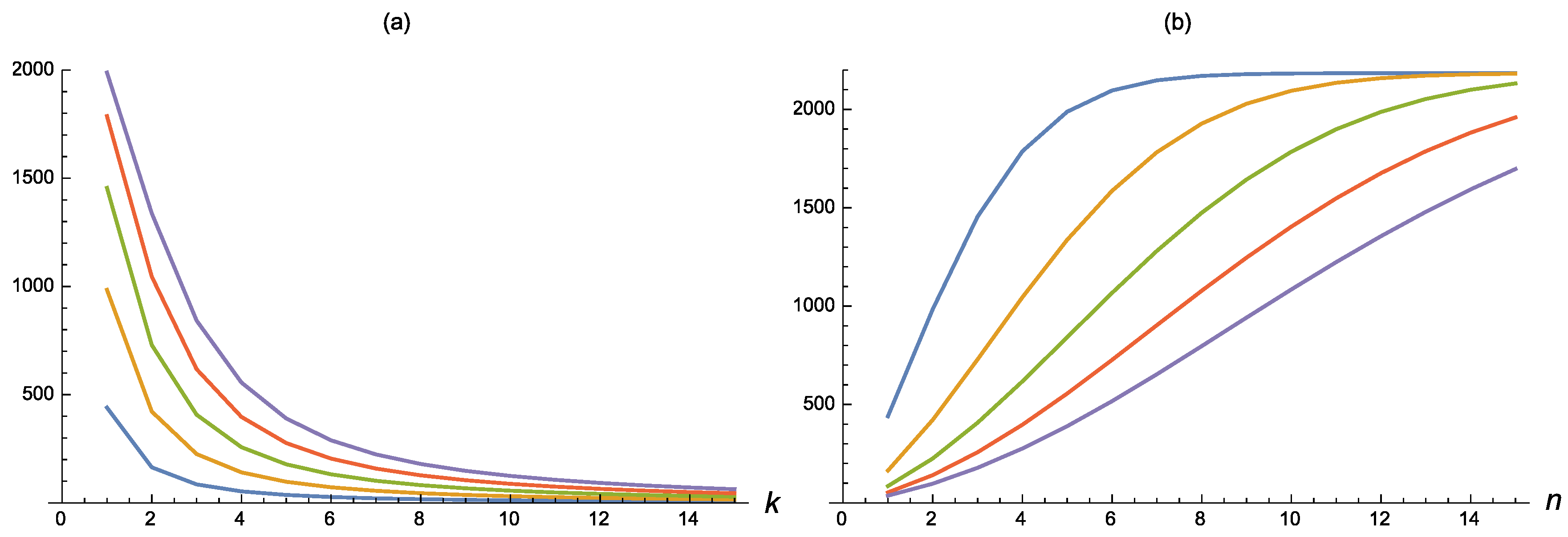
Example 2.

Consider the sample data by Abouammoh and Abdulghani [30] concerning the lifetimes (in days) of $m=40$ patients suffering from blood cancer. The evaluation of the corresponding empirical cumulative measure of inaccuracy, obtained by means of Equation (26), shows that the values of $\widehat{I}(L_{n(k)},X)$ are decreasing in k and increasing in n (see Figure 2).

Let us now discuss two special cases concerning populations from the uniform distribution and the exponential distribution.

Example 3.

Consider the random sample $X_1,X_2,\dots ,X_m$ from a population uniformly distributed in $[0,1]$. In this case, the sample spacings (27) are independent and follow the beta distribution with parameters 1 and m (for more details, see Pyke [31]). Hence, making use of (26), the mean and the variance of the empirical cumulative measure of inaccuracy are, respectively:

$$\mathbb{E}\left[\widehat{I}(L_{n(k)},X)\right]={\displaystyle \sum _{i=0}^{n-1}}{\displaystyle \sum _{j=1}^{m-1}}{\displaystyle \frac{k^i}{i!(m+1)}}{\left({\displaystyle \frac{j}{m}}\right)}^k{\left[-log\left({\displaystyle \frac{j}{m}}\right)\right]}^{i+1},$$

(28)

and

$$Var\left[\widehat{I}(L_{n(k)},X)\right]={\displaystyle \sum _{i=0}^{n-1}}{\displaystyle \sum _{j=1}^{m-1}}{\displaystyle \frac{m}{m+2}}{\left[{\displaystyle \frac{k^i}{i!(m+1)}}{\left({\displaystyle \frac{j}{m}}\right)}^k{\left[-log\left({\displaystyle \frac{j}{m}}\right)\right]}^{(i+1)}\right]}^2.$$

(29)

Table 1. Computed values of $\mathbb{E}\left[\widehat{I}(L_{n(2)},X)\right]$ and $Var\left[\widehat{I}(L_{n(2)},X)\right]$ for the uniform distribution.

	$\mathbb{E}\left[\widehat{\mathit{I}}({\mathit{L}}_{\mathit{n}(2)},\mathit{X})\right]$				$\mathit{Var}\left[\widehat{\mathit{I}}({\mathit{L}}_{\mathit{n}(2)},\mathit{X})\right]$
m	$n=2$	$n=3$	$n=4$	$n=5$	$n=2$	$n=3$	$n=4$	$n=5$
10	0.23	0.37	0.48	0.57	0.003	0.006	0.008	0.010
15	0.24	0.38	0.50	0.59	0.002	0.004	0.006	0.008
20	0.25	0.39	0.51	0.61	0.002	0.003	0.005	0.006

shows the values of the mean (28) and the variance (29) for $k=2$, and for sample sizes $m=10,15,20$, with $n=2,3,4,5$. We note that $\mathbb{E}\left[\widehat{I}(L_{n(2)},X)\right]$ is increasing in m and n.

Example 4.

Let $X_1,X_2,\dots ,X_m$ be a random sample drawn from the exponential distribution with parameter λ. Then, from (26) we see that the empirical cumulative measure of inaccuracy can be expressed as the following sum of independent and exponentially distributed random variables:

$$\widehat{I}(L_{n(k)},X)={\displaystyle \sum _{j=1}^{m-1}}{Y}_j,\mathrm{where}{Y}_j:=U_{j+1}{\displaystyle \sum _{i=0}^{n-1}}{\displaystyle \frac{k^i}{i!}}{\left({\displaystyle \frac{j}{m}}\right)}^k{\left[-log\left({\displaystyle \frac{j}{m}}\right)\right]}^{i+1}.$$

(30)

Indeed, in this case, the sample spacings $U_{j+1}$ defined in (27) are independent and exponentially distributed with mean ${\displaystyle \frac{1}{\lambda (m-j)}}$ (for more details, see Pyke [31]), so that the mean and the variance of $\widehat{I}(L_{n(k)},X)$ are given by:

$$\mathbb{E}\left[\widehat{I}(L_{n(k)},X)\right]={\displaystyle \sum _{j=1}^{m-1}}{\mu }_j,Var\left[\widehat{I}(L_{n(k)},X)\right]={\displaystyle \sum _{j=1}^{m-1}}{s}_j^2,$$

(31)

where

$${\mu }_j:=\mathbb{E}\left[Y_j\right]={\displaystyle \frac{1}{\lambda }}{\displaystyle \sum _{i=0}^{n-1}}{\displaystyle \frac{k^i}{i!(m-j)}}{\left({\displaystyle \frac{j}{m}}\right)}^k{\left[-log\left({\displaystyle \frac{j}{m}}\right)\right]}^{i+1},$$

and

$$s_j^2:=Var\left[Y_j\right]={\displaystyle \frac{1}{{\lambda }^2}}{\displaystyle \sum _{i=0}^{n-1}}{\left\{{\displaystyle \frac{k^i}{i!(m-j)}}{\left({\displaystyle \frac{j}{m}}\right)}^k{\left[-log\left({\displaystyle \frac{j}{m}}\right)\right]}^{i+1}\right\}}^2.$$

In

Table 2. Computed values of $\mathbb{E}\left[\widehat{I}(L_{n(2)},X)\right]$ and $Var\left[\widehat{I}(L_{n(2)},X)\right]$ for the exponential distribution.

	$\mathbb{E}\left[\widehat{\mathit{I}}({\mathit{L}}_{\mathit{n}(2)},\mathit{X})\right]$
$\lambda$	0.5	1	2	0.5	1	2	0.5	1	2	0.5	1	2
m		$n=2$			$n=3$			$n=4$			$n=5$
10	1.30	0.65	0.33	1.77	0.89	0.44	2.12	1.063	0.53	2.37	1.19	0.59
15	1.33	0.67	0.33	1.81	0.91	0.45	2.17	1.086	0.54	2.43	1.22	0.61
20	1.35	0.68	0.34	1.83	0.92	0.46	2.19	1.096	0.55	2.46	1.23	0.62
	$\mathit{Var}\left[\widehat{\mathit{I}}({\mathit{L}}_{\mathit{n}(\mathbf{2})},\mathit{X})\right]$
$\lambda$	0.5	1	2	0.5	1	2	0.5	1	2	0.5	1	2
m		$n=2$			$n=3$			$n=4$			$n=5$
10	0.13	0.032	0.008	0.16	0.04	0.009	0.18	0.046	0.011	0.20	0.050	0.012
15	0.09	0.022	0.005	0.11	0.028	0.007	0.12	0.031	0.008	0.14	0.035	0.008
20	0.07	0.017	0.004	0.08	0.021	0.005	0.09	0.024	0.006	0.11	0.026	0.007

, for $k=2$, we show the values of the mean and the variance (31) for sample sizes $m=10,15,20$, with $\lambda =0.5,1,2$ and $n=2,3,4,5$. One can easily see that $\mathbb{E}\left[\widehat{I}(L_{n(2)},X)\right]$ is increasing in m, whereas $Var\left[\widehat{I}(L_{n(2)},X)\right]$ is decreasing in m.

Hereafter, we show a central limit theorem for the empirical cumulative measure of inaccuracy in the same case as Example 4.

Theorem 4.

If $X_1,X_2,\dots ,X_m$ is a random sample drawn from the exponential distribution with parameter λ, then:

$${\displaystyle \frac{\widehat{I}(L_{n(k)},X)-\mathbb{E}\left[\widehat{I}(L_{n(k)},X)\right]}{{(Var\left[\widehat{I}(L_{n(k)},X)\right])}^{1/2}}}\equiv {\displaystyle \frac{{\sum }_{j=1}^{m-1}(Y_j-{\mu }_j)}{{({\sum }_{j=1}^{m-1}{s}_j^2)}^{1/2}}}\stackrel{d}{\to }\mathcal{N}(0,1).$$

Proof. 

With reference to the notation adopted in Example 4, by setting ${\alpha }_{j,r}=\mathbb{E}\left[\right|Y_j-\mathbb{E}(Y_j){|}^r]$, $r=2,3$, for large m, we have:

$$\begin{array}{lll}{\displaystyle \sum _{j=1}^{m-1}}{\alpha }_{j,2}={\displaystyle \sum _{j=1}^{m-1}}{s}_j^2\hfill & =\hfill & \frac{1}{{\lambda }^2}{\displaystyle \sum _{i=0}^{n-1}}{\left({\displaystyle \frac{k^i}{i!}}\right)}^2{\displaystyle \frac{1}{m^2}}{\displaystyle \sum _{j=1}^{m-1}}{\left\{{\displaystyle \frac{1}{(1-j/m)}}{\left({\displaystyle \frac{j}{m}}\right)}^k{\left[-log\left({\displaystyle \frac{j}{m}}\right)\right]}^{i+1}\right\}}^2\hfill \\ & \approx \hfill & {\displaystyle \frac{1}{{\lambda }^{2}m}}{\displaystyle \sum _{i=0}^{n-1}}{\left({\displaystyle \frac{k^i}{i!}}\right)}^2{c}_2^{(i,k)}\hfill \end{array}$$

and recalling that $\mathbb{E}\left[\right|Y_j-\mathbb{E}(Y_j){|}^3]=2(6-e){\left[\mathbb{E}(Y_j)\right]}^3/e$ for the exponential distribution:

$$\begin{array}{cc}{\displaystyle \sum _{j=1}^{m-1}}{\alpha }_{j,3}={\displaystyle \frac{2(6-e)}{e}}{\displaystyle \sum _{j=1}^{m-1}}{\mu }_j^3\hfill & ={\displaystyle \frac{2(6-e)}{e}}{\displaystyle \sum _{j=1}^{m-1}}{\left\{{\displaystyle \frac{1}{\lambda }}{\displaystyle \sum _{i=0}^{n-1}}{\displaystyle \frac{k^i}{i!(m-j)}}{\left({\displaystyle \frac{j}{m}}\right)}^k{\left[-log\left({\displaystyle \frac{j}{m}}\right)\right]}^{i+1}\right\}}^3\hfill \\ & \approx {\displaystyle \frac{2(6-e)}{e{\lambda }^3{m}^2}}{\left\{{\displaystyle \sum _{i=0}^{n-1}}{\displaystyle \frac{k^i}{i!}}{c}_1^{(i,k)}\right\}}^3,\hfill \end{array}$$

where

$$c_h^{(i,k)}:={\int }_0^1{\left[{\displaystyle \frac{x^k}{1-x}}{(-logx)}^{i+1}\right]}^{h}dx,h=1,2.$$

Hence, for a suitable function $C(\lambda ,i,k)$, for large m, it holds that:

$${\displaystyle \frac{{\left({\sum }_{j=1}^{m-1}{\alpha }_{j,3}\right)}^{1/3}}{{\left({\sum }_{j=1}^{m-1}{\alpha }_{j,2}\right)}^{1/2}}}\approx C(\lambda ,i,k)m^{-1/6}\to 0\mathrm{as}m\to \infty .$$

The Lyapunov’s condition of the central limit theorem is thus fulfilled, this giving the proof. □

5. Mutual Information of Lower Record Values

In this section, we study the degree of dependency between the sequences of lower record values by means of the mutual information. Recall the basic relations given in Equations (3) and (4).

First, with reference to (1), in the following theorem we obtain the entropy of k-th lower record values.

Theorem 5.

Let $\{X_n,n\ge 1\}$ be a sequence of IID random variables having finite entropy. The entropy of $L_{n(k)}$ for all $n\ge 2$ is given by:

$$H(L_{n(k)})=-logk-(n-1)\psi (n)+log((n-1)!)+n\left(1-{\displaystyle \frac{1}{k}}\right)-k^n{\phi }_f(n-1),$$

(32)

where $\psi (n)={\Gamma }^{\prime }(n)/\Gamma (n)$ is the digamma function, and:

$${\phi }_f(n-1):={\int }_0^{+\infty }{\displaystyle \frac{z^{n-1}}{(n-1)!}}{e}^{-zk}log(f(F^{-1}(e^{-z})))dz.$$

(33)

Proof. 

As customary, we denote by $f(x)$ and $F(x)$ the PDF and CDF of $X_1$. By (7), we have:

$$\begin{array}{cc}\hfill H(L_{n(k)})& =-{\int }_{-\infty }^{+\infty }{f}_{n(k)}(x)log(f_{n(k)}(x))dx\hfill \\ & =-{\int }_{-\infty }^{+\infty }{\displaystyle \frac{k^n}{(n-1)!}}{\left[F(x)\right]}^{k-1}{\left[\tilde{\Lambda }(x)\right]}^{n-1}f(x)log\left({\displaystyle \frac{k^n}{(n-1)!}}{\left[F(x)\right]}^{k-1}{\left[\tilde{\Lambda }(x)\right]}^{n-1}f(x)\right)dx\hfill \\ & =-{\displaystyle \frac{k^n}{(n-1)!}}{\int }_{-\infty }^{+\infty }\{n{\left[\tilde{\Lambda }(x)\right]}^{n-1}{\left[F(x)\right]}^{k-1}f(x)logk+(n-1){\left[\tilde{\Lambda }(x)\right]}^{n-1}{\left[F(x)\right]}^{k-1}f(x)log(\tilde{\Lambda }(x))\hfill \\ & +(k-1){\left[\tilde{\Lambda }(x)\right]}^{n-1}{\left[F(x)\right]}^{k-1}f(x)log(F(x))+{\left[\tilde{\Lambda }(x)\right]}^{n-1}{\left[F(x)\right]}^{k-1}f(x)log(f(x))\hfill \\ & -{\left[\tilde{\Lambda }(x)\right]}^{n-1}{\left[F(x)\right]}^{k-1}f(x)log((n-1)!)\}dx.\hfill \end{array}$$

By taking $z=\tilde{\Lambda }(x)$, we get:

$$\begin{array}{cc}\hfill H(L_{n(k)})& =-k^n{\int }_0^{+\infty }[n{\displaystyle \frac{z^{n-1}}{(n-1)!}}{e}^{-zk}logk+{\displaystyle \frac{z^{n-1}}{(n-2)!}}{e}^{-zk}logz\hfill \\ & -(k-1){\displaystyle \frac{z^n}{(n-1)!}}{e}^{-zk}+{\displaystyle \frac{z^{n-1}}{(n-1)!}}{e}^{-zk}log(f(F^{-1}(e^{-z})))-{\displaystyle \frac{z^{n-1}}{(n-1)!}}{e}^{-zk}log((n-1)!)]dz.\hfill \end{array}$$

Hence, making use of Equation (A.8) of Zahedi and Shakil [32], after some calculations we finally get: Equation (32). □

It is worth noting the analogies between Equation (33) and the function ${\varphi }_f(n)$ considered by Baratpour et al. [33] for the analysis of the upper record values.

In the following lemma we express the mutual information between $Z_{m(k)}$ and $Z_{n(k)}$ in terms of the digamma function.

Lemma 1.

Let $Z_{n(k)}$ be the k-th lower record values from the uniform distribution over interval $(0,1)$. Then, the mutual information between $Z_{m(k)}$ and $Z_{n(k)}$, for $n>m$, is given by:

$$\begin{array}{cc}\hfill M(Z_{m(k)},Z_{n(k)})& =m+log((n-1)!)-log((n-m-1)!)\hfill \\ & +(n-m-1)\psi (n-m)-(n-1)\psi (n).\hfill \end{array}$$

Proof. 

In this case, recalling (9), we have $\tilde{\Lambda }(x)=-logx$, $0<x<1$. Hence, making use of Equations (2), (4), (8) and (10), for $n>m$ we get:

$$\begin{array}{cc}\hfill H(Z_{n(k)}|Z_{m(k)})& =-{\int }_0^1{\int }_0^x{\displaystyle \frac{k^n{[-log(y)+log(x)]}^{n-m-1}{[-log(x)]}^{m-1}{y}^{k-1}}{(m-1)!(n-m-1)!x}}\hfill \\ & \times log\left[{\displaystyle \frac{k^n{y}^{k-1}}{k^m{x}^k}}{\displaystyle \frac{{[-log(y)+log(x)]}^{n-m-1}}{(n-m-1)!}}\right]dydx\hfill \\ & ={\displaystyle \sum _{r=1}^5}{I}_r,\hfill \end{array}$$

(34)

where

$$\begin{array}{cc}\hfill I_1& :=-(n-m)log(k){\int }_0^1{\int }_0^x{f}_{m(k),n(k)}(x,y)dydx=(n-m)log(k),\hfill \\ \hfill I_2& :=log[(n-m-1)!]{\int }_0^1{\int }_0^x{f}_{m(k),n(k)}(x,y)dydx=log[(n-m-1)!],\hfill \\ \hfill I_3& :={\int }_0^1{\int }_0^x{\displaystyle \frac{k^{n+1}{[-log(y)+log(x)]}^{n-m-1}{[-log(x)]}^{m-1}{y}^{k-1}}{(m-1)!(n-m-1)!x}}log(x)dydx=-m,\hfill \\ \hfill I_4& :=-{\int }_0^1{\int }_0^x{\displaystyle \frac{k^n{[-log(y)+log(x)]}^{n-m-1}{[-log(x)]}^{m-1}{y}^{k-1}}{(m-1)!(n-m-1)!x}}log{[-log(y)+log(x)]}^{n-m-1}dydx\hfill \\ & =-(n-m-1)[\psi (n-m)-log(k)],\hfill \\ \hfill I_5& :=-{\int }_0^1{\int }_0^x{\displaystyle \frac{(k-1)k^n{[-log(y)+log(x)]}^{n-m-1}{[-log(x)]}^{m-1}{y}^{k-1}}{(m-1)!(n-m-1)!x}}log(y)dydx=n\left(1-{\displaystyle \frac{1}{k}}\right).\hfill \end{array}$$

Hence, by straightforward calculations we obtain:

$$H(Z_{n(k)}|Z_{m(k)})=log((n-m-1)!)-(n-m)log(k)-(n-m-1)[\psi (n-m)-logk]+{\displaystyle \frac{k-1}{k}}(n-2m)-m,$$

(35)

where $\psi (n-m)={\int }_0^{+\infty }{t}^{n-m}{e}^{-t}log(t)dt$. Similarly, by (32) we have

$$H(Z_{n(k)})=-logk-(n-1)\psi (n)+log((n-1)!)+n\left(1-{\displaystyle \frac{1}{k}}\right).$$

(36)

Recalling (4), the thesis thus follows from (35) and (36). □

Let us now come to the main result of this section. Recall that the mutual information of $(X,Y)$ is defined in (3).

Theorem 6.

Under the assumptions of Theorem 5, the following result holds:

(i) 

The mutual information between the m-th and the n-th k-lower records is distribution-free, and is given by:

$$\begin{array}{cc}\hfill M(L_{m(k)},L_{n(k)})& =m+log((n-1)!)-log((n-m-1)!)\hfill \\ & +(n-m-1)\psi (n-m)-(n-1)\psi (n).\hfill \end{array}$$

(37)

(ii) 

The mutual information $M(L_{m(k)},L_{m+1(k)})$ is increasing in m.

Proof. 

(i)

Let $Z_{m(k)}=F^{-1}(L_{m(k)})$ and $Z_{n(k)}=F^{-1}(L_{n(k)})$, where $F^{-1}$ denotes the pseudo-inverse function of F, i.e., the quantile function of X. Then, $Z_{m(k)}$ and $Z_{n(k)}$ are the m-th and n-th k-lower records of the uniform distribution over the interval $(0,1)$. By the invariance property of mutual information, we have: $M(L_{m(k)},L_{n(k)})=M(Z_{m(k)},Z_{n(k)})$, thus the result follows from Lemma 1.

(ii)

By taking $n=m+1$ in (37), we get:

$$M(L_{m(k)},L_{m+1(k)})=m+log(m!)-m\psi (m+1),$$

so that

$$\begin{array}{cc}\hfill M(L_{m+1(k)},L_{m+2(k)})-M(L_{m(k)},L_{m+1(k)})& =log((m+1)!)-log(m!)\hfill \\ & +m\psi (m+1)-(m+1)\psi (m+2)+1.\hfill \end{array}$$

It is not hard to see that the right-hand-side is positive, and the proof thus follows. □

It is useful to assess the mutual information between the k-th lower record values, such as when such values correspond to successive failures of a repairable system. Hence, the information provided in Theorem 6 is useful for constructing suitable replacement criteria of components, in order to avoid failures and to improve system availability.

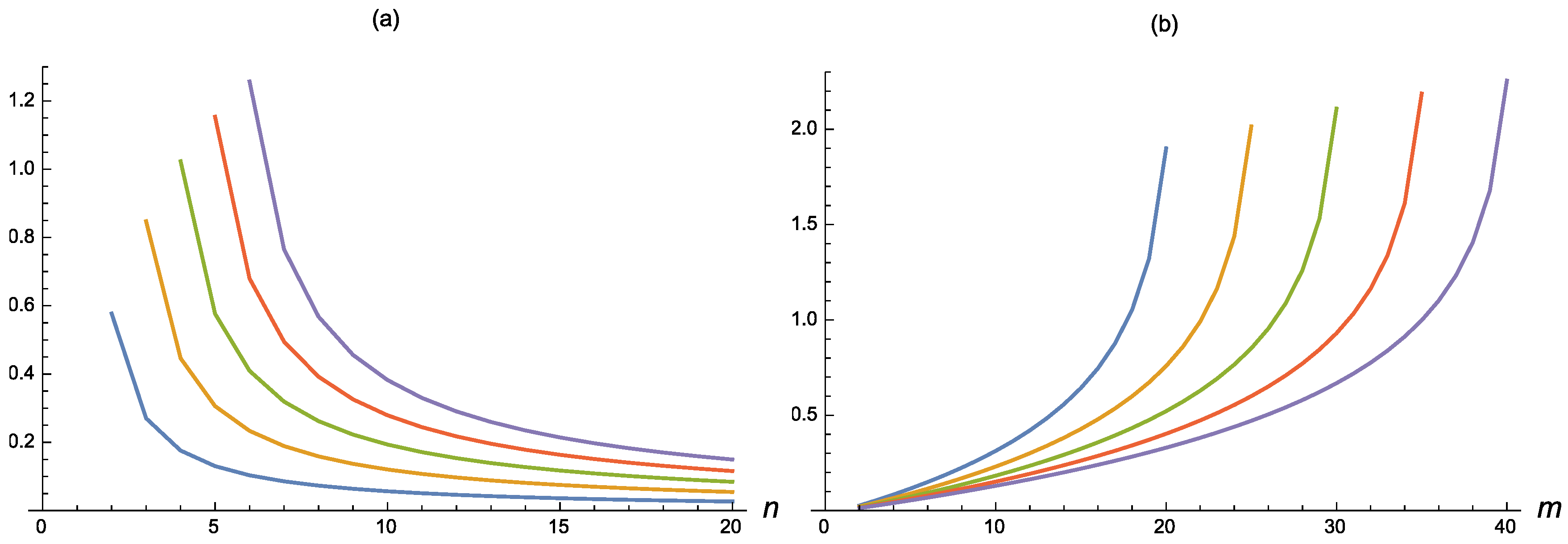
The mutual information between the m-th and the n-th k-lower records, determined in Equation (37), is shown in Figure 3 for different choices of m and n. For fixed values of m, such an information measure is decreasing in n, whereas for fixed n, it is increasing in m.

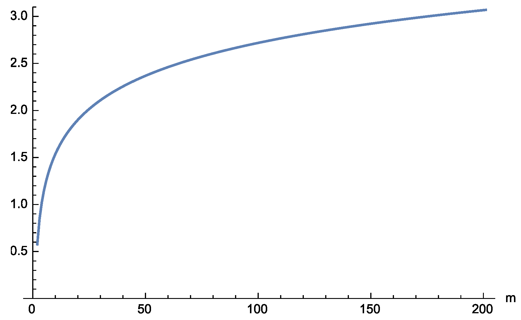
Finally, Figure 4 shows that $M(L_{m(k)},L_{m+1(k)})$ is increasing in m, in agreement with the point (ii) of Theorem 6.

6. Conclusions

In this paper, we discussed the concept of inaccuracy between $L_{n(k)}$ and X in a random sample generated by X. We proposed a dynamic version of cumulative inaccuracy and studied a related characterization result. We also proved that $I(L_{n(k)},X;t)$ can uniquely determine the parent distribution F. Moreover, we constructed bounds for characterization results of $I(L_{n(k)},X)$. Also, we estimated the cumulative measure of inaccuracy by means of the empirical cumulative inaccuracy in lower record values. These concepts can be applied in measuring the inaccuracy contained in the associated past lifetime. Finally, we studied the degree of dependency among the sequence of k-th lower record values in terms of mutual information. We showed that $M(L_{m(k)},L_{n(k)})$ is distribution-free and can be computed by using the distribution of the k-th lower record values of the sequence from the uniform distribution.