Spectra of Subdivision Vertex-Edge Join of Three Graphs

Abstract

In this paper, we introduce a new graph operation called subdivision vertex-edge join (denoted by $G_1^S▹(G_2^V\cup G_3^E)$ for short), and then the adjacency spectrum, the Laplacian spectrum and the signless Laplacian spectrum of $G_1^S▹(G_2^V\cup G_3^E)$ are respectively determined in terms of the corresponding spectra for a regular graph $G_1$ and two arbitrary graphs $G_2$ and $G_3$. All the above can be viewed as the generalizations of the main results in [X. Liu, Z. Zhang, Bull. Malays. Math. Sci. Soc., 2017:1–17]. Furthermore, we also determine the normalized Laplacian spectrum of $G_1^S▹(G_2^V\cup G_3^E)$ whenever $G_i$ are regular graphs for each index $i=1,2,3$. As applications, we construct infinitely many pairs of A-cospectral mates, L-cospectral mates, Q-cospectral mates and $\mathcal{L}$-cospectral mates. Finally, we give the number of spanning trees, the (degree-)Kirchhoff index and the Kemeny’s constant of $G_1^S▹(G_2^V\cup G_3^E)$, respectively.

1. Introduction

All graphs considered in this paper are undirected and simple. Let $G=(V,E)$ be a graph with $V\left(G\right)=\{v_1,v_2,\dots ,v_n\}$ and $E\left(G\right)=\{e_1,e_2,\dots ,e_m\}$, where $\left|V\right(G\left)\right|=n$ and $\left|E\right(G\left)\right|=m$. We denote by $d_i=d_G\left(v_i\right)$ the degree of $v_i$ in G, and define $A\left(G\right)$ and $D\left(G\right)$ to be the adjacency matrix and the degree diagonal matrix, respectively.

A graph matrix $M=M\left(G\right)$ is a symmetric matrix with respect to adjacency matrix $A\left(G\right)$ of G. As usual, M is separately called the adjacency matrix, the Laplacian matrix, the signless Laplacian matrix and the normalized Laplacian matrix of G if M equals $A\left(G\right)$, $L\left(G\right)=D\left(G\right)-A\left(G\right)$, $Q\left(G\right)=D\left(G\right)+A\left(G\right)$ and $\mathcal{L}\left(G\right)=D^{-1/2}\left(G\right)(D\left(G\right)-A\left(G\right))D^{-1/2}\left(G\right)=I-D^{-1/2}\left(G\right)A\left(G\right)D^{-1/2}\left(G\right)$. The M-characteristic polynomial of G is defined as ${\mathsf{\Phi }}_M\left(\lambda \right)=det(\lambda I-M)$. Since M is real symmetric, its eigenvalues are real number. The M-spectrum, denoted by $Spe{c}_M\left(G\right)$, of G is a multiset consisting of the M-eigenvalues. The A-eigenvalues, L-eigenvalues, Q-eigenvalues and $\mathcal{L}$-eigenvalues are respectively arranged as ${\theta }_1\le {\theta }_2\le \cdots \le {\theta }_n$, $0={\eta }_1\le {\eta }_2\le \cdots \le {\eta }_n$, ${\mu }_1\le {\mu }_2\le \cdots \le {\mu }_n$ and $0={\nu }_1\le {\nu }_2\le \cdots \le {\nu }_n\le 2$. Graphs G and H are said to be M-cospectral if they share the same M-spectrum. An M-cospectral mate of G is a graph cospectral with but not isomorphic to G, and G is said to be determined by its M-spectrum if any graph H that is M-cospectral with G is also isomorphic to G. Furthermore, the line graph $\ell \left(G\right)$ of graph G is a graph whose vertices corresponding the edges of G, and where two vertices are adjacent iff the corresponding edges of G are adjacent. Let $K_n$, $K_{m,n}$ and $P_n$ denote the complete graph, the complete bipartite graph and the path, respectively.

The spectra of a graph provide information on its structural properties and also on some relevant dynamical aspects [1,2]. Calculating the spectra of graphs as well as formulating the characteristic polynomials of graphs is a fundamental and very meaningful work in spectral graph theory. Moreover, those allow the calculation of some interesting graph invariants such as the number of spanning trees [3,4,5,6], the (degree-)Kirchhoff index [7] and the Kemeny’s constant [8] and so on. Up till now, many graph operations such as the disjoint union, the corona [9], the edge corona [10,11], the neighborhood corona [12] and the subdivision vertex (edge) neighborhood corona [13] have been introduced, and their spectra are computed respectively. 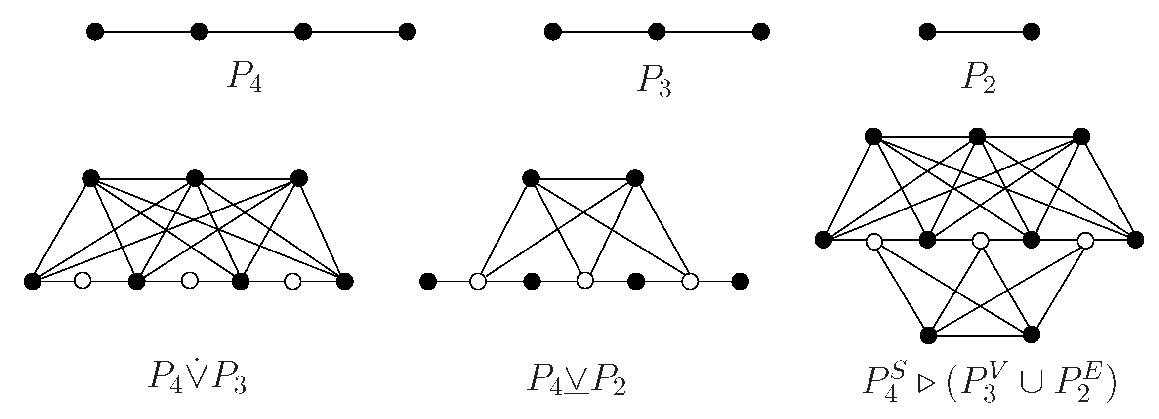Recently, many researchers have concerned the subdivision-join of two graphs. Indulal [14] introduced two new joins subdivision vertex-join $G_1\dot{\vee }{G}_2$ and subdivision edge-join $G_1⊻G_2$ (for example, we depict $P_4\dot{\vee }{P}_3$ and $P_4⊻P_2$ in Figure 1 if $G_1=P_4$ and $G_2=P_3$, or $P_2$), and their A-spectra are investigated when $G_1$ and $G_2$ are both regular graphs. In [15], Liu and Zhang have determined the adjacency, the Laplacian and the signless Laplacian spectra of $G_1\dot{\vee }{G}_2$ and $G_1⊻G_2$ for a regular graph $G_1$ and an arbitrary graph $G_2$.

Figure 1. Some related graphs.

Inspired by above, we introduce a new graph operation based on subdivision and join. For a graph $G_1$, let $S\left(G_1\right)$ be the subdividing graph of $G_1$ whose vertex set has two parts: one the origin vertices $V\left(G_1\right)$, another, denoted by $I\left(G_1\right)$, the inserting vertices corresponding to the edges of $G_1$. Let $G_2$ and $G_3$ be other two disjoint graphs. Then we have the following definition.

Definition 1.

The subdivision vertex-edge join (short for SVE-join) of $G_1$ with $G_2$ and $G_3$, denoted by $G_1^S▹(G_2^V\cup G_3^E)$, is the graph consisting of $S\left(G_1\right)$, $G_2$ and $G_3$, all vertex-disjoint, and joining the i-th vertex of $V\left(G_1\right)$ to every vertex in the $V\left(G_2\right)$ and i-th vertex of $I\left(G_1\right)$ to each vertex in the $V\left(G_3\right)$.

For instance, we depict $G_1^S▹(G_2^V\cup G_3^E)$ in the following Figure 1 if $G_1=P_4,G_2=P_3$ and $G_3=P_2$.

It is easy to see that $G_1^S▹(G_2^V\cup G_3^E)$ has $n=n_1+m_1+n_2+n_3$ vertices and $m=2m_1+n_1{n}_2+m_1{n}_3+m_2+m_3$ edges, where $n_i$ and $m_i$ are the number of vertices and edges of $G_i$ for $i=1,2,3$. Also, we see that $G_1^S▹(G_2^V\cup G_3^E)$ is $G_1\dot{\vee }{G}_2$ (see [14]) if $G_3$ is the null graph, and is $G_1⊻G_3$ (see [14]) if $G_2$ is the null graph.

In this paper, we respectively determine the adjacency, the Laplacian and the signless Laplacian spectrum of $G_1^S▹(G_2^V\cup G_3^E)$ for a regular graph $G_1$ and two arbitrary graph $G_2$ and $G_3$ in terms of the corresponding spectra for a regular graph $G_1$ and two arbitrary graphs $G_2$ and $G_3$. All the above can be viewed as the generalizations of the main results in [15]. In addition, we also determine the normalized Laplacian spectrum of $G_1^S▹(G_2^V\cup G_3^E)$ whenever $G_1$, $G_2$ and $G_3$ are regular graphs.

“Which graph is determined by its spectrum?” [16] is a long-standing open problem in the theory of graph spectra. The problem was first raised in 1956 by Günthard and Primas [17], which relates the theory of graph spectra to Hückel’s theory from chemistry. Showing graphs to be determined by their spectra or constructing as many as cospectral non-isomorphic graphs (i.e., cospectral mates) are two sides of one coin, and both providing valuable insights to understanding the above open question. As an application of our main results (See Theorems 1–4), we focus the later and construct infinitely many pairs of M-cospectral mates ($M=A,L,Q,\mathcal{L}$) since M-cospectral mates have the same M-characteristic polynomials, and SVE-join whose corresponding M-characteristic polynomials are known. Subsequently, we give the number of spanning trees, the (degree-)Kirchhoff index and the Kemeny’s constant of $G_1^S▹(G_2^V\cup G_3^E)$, respectively.

The paper is organized as follows. In Section 2, we give some preliminary results that will be needed in later in the paper. In Section 3, we present $A,L,Q,\mathcal{L}$-characteristic polynomials and their corresponding spectra of $G_1^S▹(G_2^V\cup G_3^E)$. Some applications are given in Section 4.

2. Elementary

In this section, we give some useful established results which are required in the proof of the main result.

Lemma 1 

([18]). For a graph G with n vertices and m edges, let $R\left(G\right)$ and $\ell \left(G\right)$ be the incidence matrix of G and the line graph of G, respectively. Then

$$R{\left(G\right)}^{T}R\left(G\right)=2I_m+A\left(\ell \left(G\right)\right),R\left(G\right)R{\left(G\right)}^T=Q\left(G\right).$$

Corollary 1 

([18]). If G is an r-regular graph. Then

(a)

${\mathsf{\Phi }}_{A\left(\ell \right(G\left)\right)}\left(\lambda \right)={(\lambda +2)}^{m-n}·{\displaystyle \prod _{i=1}^n}(\lambda -(r-2)-{\theta }_i\left(G\right))$;

(b)

${\mathsf{\Phi }}_{A\left(\ell \right(G\left)\right)}\left(\lambda \right)={(\lambda +2)}^{m-n}·{\displaystyle \prod _{i=1}^n}(\lambda -(2r-2)+{\eta }_i\left(G\right))$;

(c)

${\mathsf{\Phi }}_{A\left(\ell \right(G\left)\right)}\left(\lambda \right)={(\lambda +2)}^{m-n}·{\displaystyle \prod _{i=1}^n}(\lambda +2-{\mu }_i\left(G\right))$;

(d)

${\mathsf{\Phi }}_{A\left(\ell \right(G\left)\right)}\left(\lambda \right)={(\lambda +2)}^{m-n}·{\displaystyle \prod _{i=1}^n}(\lambda -(2r-2)+r{\nu }_i\left(G\right))$

where ${\theta }_i\left(G\right)$, ${\eta }_i\left(G\right)$, ${\mu }_i\left(G\right)$ and ${\nu }_i\left(G\right)$ are the eigenvalues of $A\left(G\right)$, $L\left(G\right)$, $Q\left(G\right)$ and $\mathcal{L}\left(G\right)$, respectively.

Corollary 2.

Let G be an r-regular graph with n vertices and m edges. For a constant a, we have

(i)

$R\left(G\right){(\lambda I_m-a{J}_{m\times m})}^{-1}R{\left(G\right)}^T=\frac{r{I}_n+A\left(G\right)}{\lambda }+\frac{a{r}^2{J}_{n\times n}}{\lambda (\lambda -ma)}$;

(ii)

$R{\left(G\right)}^T{(\lambda I_n-a{J}_{n\times n})}^{-1}R\left(G\right)=\frac{2I_m+A\left(\ell \left(G\right)\right)}{\lambda }+\frac{4a{J}_{m\times m}}{\lambda (\lambda -na)}$

where $I_m$ is identity matrix and $J_{n\times n}$ is matrix of size $n\times n$ with all entries equal to one.

Proof. 

Please note that G is an r-regular graph. Then by Lemma 1 we have $R\left(G\right)R{\left(G\right)}^T=r{I}_n+A\left(G\right)$. Therefore,

$$\begin{array}{cc}\hfill R\left(G\right){(\lambda I_m-a{J}_{m\times m})}^{-1}R{\left(G\right)}^T& =\frac{R\left(G\right)((\lambda -ma)I_m+a{J}_{m\times m})R{\left(G\right)}^T}{\lambda (\lambda -ma)}\hfill \\ \hfill & =\frac{(\lambda -ma)R\left(G\right)R{\left(G\right)}^T+aR\left(G\right)J_{m\times m}R{\left(G\right)}^T}{\lambda (\lambda -ma)}\hfill \\ & =\frac{r{I}_n+A\left(G\right)}{\lambda }+\frac{a{r}^2{J}_{n\times n}}{\lambda (\lambda -ma)}.\hfill \end{array}$$

Similarly, (ii) can be verified. □

Lemma 2 

([19]). Let $M_1$, $M_2$, $M_3$, $M_4$ be respectively $p\times p$, $p\times q$, $q\times p$, $q\times q$ matrices with $M_1$ and $M_4$ invertible. Then

$$\begin{array}{cc}\hfill det\left(\begin{array}{cc}\hfill M_1& M_2\hfill \\ \hfill M_3& M_4\hfill \end{array}\right)& =det\left(M_4\right)·det(M_1-M_2{M}_4^{-1}{M}_3)\hfill \\ & =det\left(M_1\right)·det(M_4-M_3{M}_1^{-1}{M}_2).\hfill \end{array}$$

where $M_1-M_2{M}_4^{-1}{M}_3$ and $M_4-M_3{M}_1^{-1}{M}_2$ are called the Schur complements of $M_4$ and $M_1$.

For two matrices $A={\left(a_{ij}\right)}_{m\times n}$ and $B={\left(b_{ij}\right)}_{m\times n}$, the Hadamard product $A•B$ is a matrix of size $m\times n$ with entries ${(A•B)}_{ij}=a_{ij}·b_{ij}$, which is given by [20].

For a matrix M of order n, we respectively denote by ${\mathbf{1}}_n$ and $J_{m\times n}$ the column vector of size n and the matrix of size $m\times n$ with all the entries equal one. M-coronal ${\Gamma }_M\left(\lambda \right)$ is defined, in [21], to be the sum of the entries of the matrix ${(\lambda I-M)}^{-1}$, i.e.,

$${\Gamma }_M\left(\lambda \right)={\mathbf{1}}_n^T{(\lambda I_n-M)}^{-1}{\mathbf{1}}_n.$$

If M has constant row sum t, it is easy to verify that

$${\Gamma }_M\left(\lambda \right)=\frac{n}{\lambda -t}.$$

Lemma 3 

([15]). Let A ba an $n\times n$ real matrix, and adj(A) denote the adjugated matrix of A. Then

$$det(A+a{J}_{n\times n})=det\left(A\right)+a{\mathbf{1}}_n^{T}adj\left(A\right){\mathbf{1}}_n,$$

Moreover,

$$det(\lambda I_n-A-a{J}_{n\times n})=(1-a{\Gamma }_A\left(\lambda \right))det(\lambda I_n-A).$$

3. Spectra of SVE-join

Let $G_i$ be a graph with $n_i$ vertices and $m_i$ edges for each index $i=1,2,3$. For the graph $G=G_1^S▹(G_2^V\cup G_3^E)$, we first label its vertices in the following: $V\left(G_1\right)=\{v_1,v_2,\dots ,v_{n_1}\}$, $I\left(G_1\right)=\{e_1,e_2,\dots ,e_{m_1}\}$, $V\left(G_2\right)=\{u_1,u_2,\dots ,u_{n_2}\}$ and $V\left(G_3\right)=\{w_1,w_2,\dots ,w_{n_3}\}$. Then the vertices of G is partitioned by

$$V\left(G\right)=V\left(G_1\right)\cup I\left(G_1\right)\cup V\left(G_2\right)\cup V\left(G_3\right).$$

(1)

From Definition 1, the degrees of the vertices of G are:

$$\begin{array}{c}{d}_G\left(v\right)=\left\{\begin{array}{cc}2+n_3\hfill & \mathrm{if}v\in I\left(G_1\right);\hfill \\ d_{G_1}\left(v_i\right)+n_2\hfill & \mathrm{if}v\in V\left(G_1\right),i=1,2,\dots ,n_1;\hfill \\ d_{G_2}\left(u_j\right)+n_1\hfill & \mathrm{if}v\in V\left(G_2\right),j=1,2,\dots ,n_2;\hfill \\ d_{G_3}\left(w_k\right)+m_1\hfill & \mathrm{if}v\in V\left(G_3\right),k=1,2,\dots ,n_3.\hfill \end{array}\right.\end{array}$$

(2)

Those above will be persisted in what follows.

3.1. A-spectrum, L-spectrum and Q-spectrum of SVE-join

In this section, we focus on determining the A-spectrum, L-spectrum and Q-spectrum of subdivision vertex-edge join $G_1^S▹(G_2^V\cup G_3^E)$ whenever $G_1$ is $r_1$-regular graph.

Theorem 1.

Let $G_1$ be an $r_1$-regular graph with $n_1$ vertices and $m_1$ edges, and $G_i$ be arbitrary graphs on $n_i$ vertices for each index $i=2,3$. Then $G=G_1^S▹(G_2^V\cup G_3^E)$ has A-characteristic polynomial

$$\begin{array}{cc}\hfill {\mathsf{\Phi }}_{A\left(G\right)}\left(\lambda \right)& ={\mathsf{\Phi }}_{A\left(G_2\right)}\left(\lambda \right)·{\mathsf{\Phi }}_{A\left(G_3\right)}\left(\lambda \right)·{\displaystyle \prod _{i=1}^{n_1-1}}({\lambda }^2-r_1-{\theta }_i\left(G_1\right))\hfill \\ & \times {\lambda }^{m_1-n_1}·\left({\lambda }^2-(n_1{\Gamma }_{A\left(G_2\right)}\left(\lambda \right)+m_1{\Gamma }_{A\left(G_3\right)}\left(\lambda \right))\lambda +m_1{n}_1{\Gamma }_{A\left(G_2\right)}\left(\lambda \right){\Gamma }_{A\left(G_3\right)}\left(\lambda \right)-2r_1\right).\hfill \end{array}$$

Proof. 

Let $R\left(G_1\right)$ be the adjacency matrix of $G_1$. The adjacency matrix of G can be represented in the form of block-matrix according to the partition (1) as follows:

$$A\left(G\right)=\left(\begin{array}{cccc}{O}_{n_1\times n_1}& R\left(G_1\right)& J_{n_1\times n_2}& O_{n_1\times m_3}\\ R{\left(G_1\right)}^T& O_{m_1\times m_1}& O_{m_1\times n_2}& J_{m_1\times n_3}\\ J_{n_2\times n_1}& O_{n_2\times m_1}& A\left(G_2\right)& O_{n_2\times n_3}\\ O_{n_3\times n_1}& J_{n_3\times m_1}& O_{n_3\times n_2}& A\left(G_3\right)\end{array}\right).$$

(3)

Then the characteristic polynomial of G is obtained from Equation (3) as follows

$$\begin{array}{cc}\hfill {\mathsf{\Phi }}_{A\left(G\right)}\left(\lambda \right)& =|\lambda I_n-A\left(G\right)|\hfill \\ \hfill & =\left|\begin{array}{cccc}\lambda I_{n_1}& -R\left(G_1\right)& -J_{n_1\times n_2}& O\\ -R{\left(G_1\right)}^T& \lambda I_{m_1}& O& -J_{m_1\times n_3}\\ -J_{n_2\times n_1}& O& \lambda I_{n_2}-A\left(G_2\right)& O\\ O& -J_{n_3\times m_1}& O& \lambda I_{n_3}-A\left(G_3\right)\end{array}\right|\hfill \\ \hfill & =\left|\begin{array}{cccc}\lambda I_{n_1}-{\Gamma }_{A\left(G_2\right)}\left(\lambda \right)J_{n_1\times n_1}& -R\left(G_1\right)& 0& O\\ -R{\left(G_1\right)}^T& \lambda I_{m_1}-{\Gamma }_{A\left(G_3\right)}\left(\lambda \right)J_{m_1\times m_1}& O& 0\\ -J_{n_2\times n_1}& O& \lambda I_{n_2}-A\left(G_2\right)& O\\ O& -J_{n_3\times m_1}& O& \lambda I_{n_3}-A\left(G_3\right)\end{array}\right|\hfill \\ & =|\lambda I_{n_2}-A\left(G_2\right)|·|\lambda I_{n_3}-A\left(G_3\right)|·det\left(S_1\right),\hfill \end{array}$$

where

$$\begin{array}{cc}\hfill S_1& =\left(\begin{array}{cc}\lambda I_{n_1}-{\Gamma }_{A\left(G_2\right)}\left(\lambda \right)J_{n_1\times n_1}& -R\left(G_1\right)\\ -R{\left(G_1\right)}^T& \lambda I_{m_1}-{\Gamma }_{A\left(G_3\right)}\left(\lambda \right)J_{m_1\times m_1}\end{array}\right).\hfill \end{array}$$

By Corollary 2, Lemmas 2 and 3, we have

$$\begin{array}{cc}\hfill det\left(S_1\right)& =det(\lambda I_{m_1}-{\Gamma }_{A\left(G_3\right)}\left(\lambda \right)J_{m_1\times m_1}-R{\left(G_1\right)}^T{(\lambda I_{n_1}-{\Gamma }_{A\left(G_2\right)}\left(\lambda \right)J_{n_1\times n_1})}^{-1}R\left(G_1\right))\hfill \\ \hfill & \times det(\lambda I_{n_1}-{\Gamma }_{A\left(G_2\right)}\left(\lambda \right)J_{n_1\times n_1})\hfill \\ \hfill & =det(\lambda I_{m_1}-{\Gamma }_{A\left(G_3\right)}\left(\lambda \right)J_{m_1\times m_1}-\frac{2I_{m_1}+A\left(\ell \left(G_1\right)\right)}{\lambda }-\frac{4{\Gamma }_{A\left(G_2\right)}\left(\lambda \right)J_{m_1\times m_1}}{\lambda (\lambda -n_1{\Gamma }_{A\left(G_2\right)}\left(\lambda \right))})\hfill \\ \hfill & \times det(\lambda I_{n_1}-{\Gamma }_{A\left(G_2\right)}\left(\lambda \right)J_{n_1\times n_1})\hfill \\ \hfill & =(1-(\frac{4{\Gamma }_{A\left(G_2\right)}\left(\lambda \right)}{\lambda (\lambda -n_1{\Gamma }_{A\left(G_2\right)}\left(\lambda \right))}+{\Gamma }_{A\left(G_3\right)}\left(\lambda \right)){\Gamma }_{\frac{2I_{m_1}+A\left(\ell \left(G_1\right)\right)}{\lambda }}\left(\lambda \right))·det(\lambda I_{m_1}-\frac{2I_{m_1}+A\left(\ell \left(G_1\right)\right)}{\lambda })\hfill \\ & \times det(\lambda I_{n_1}-{\Gamma }_{A\left(G_2\right)}\left(\lambda \right)J_{n_1\times n_1})\hfill \end{array}$$

(4)

From Lemma 3, we get

$$\begin{array}{cc}\hfill det(\lambda I_{n_1}-{\Gamma }_{A\left(G_2\right)}\left(\lambda \right)J_{n_1\times n_1})& =(1-{\Gamma }_{A\left(G_2\right)}\left(\lambda \right){\Gamma }_O\left(\lambda \right))·det\left(\lambda I_{n_1}\right)\hfill \\ \hfill & ={\lambda }^{n_1}(1-{\Gamma }_{A\left(G_2\right)}\left(\lambda \right)·\frac{n_1}{\lambda })\hfill \\ & ={\lambda }^{n_1}-n_1{\Gamma }_{A\left(G_2\right)}\left(\lambda \right){\lambda }^{n_1-1}.\hfill \end{array}$$

(5)

Moreover, the sum of all entries on every row of matrix $\frac{2I_{m_1}+A\left(\ell \left(G_1\right)\right)}{\lambda }$ is $\frac{2r_1}{\lambda }$, thus

$${\Gamma }_{\frac{2I_{m_1}+A\left(\ell \left(G_1\right)\right)}{\lambda }}\left(\lambda \right)=\frac{m_1}{\lambda -\frac{2r_1}{\lambda }}=\frac{m_1\lambda }{{\lambda }^2-2r_1}.$$

(6)

Since $G_1$ is an $r_1$-regular graph, ${\theta }_{n_1}\left(G_1\right)=r_1$. From Corollary 1 (a), we know that the eigenvalues of $A\left(\ell \left(G_1\right)\right)$ are the eigenvalues of $(r_1-2)I_{n_1}+A\left(G_1\right)$ and $-2$ repeated $m_1-n_1$ times. Combining Equations (4)–(6), we have

$$\begin{array}{cc}\hfill det\left(S_1\right)& =(1-(\frac{4{\Gamma }_{A\left(G_2\right)}\left(\lambda \right)}{\lambda (\lambda -n_1{\Gamma }_{A\left(G_2\right)}\left(\lambda \right))}+{\Gamma }_{A\left(G_3\right)}\left(\lambda \right)){\Gamma }_{\frac{2I_{m_1}+A\left(\ell \left(G_1\right)\right)}{\lambda }}\left(\lambda \right))·det(\lambda I_{m_1}-\frac{2I_{m_1}+A\left(\ell \left(G_1\right)\right)}{\lambda })\hfill \\ \hfill & \times det(\lambda I_{n_1}-{\Gamma }_{A\left(G_2\right)}\left(\lambda \right)J_{n_1\times n_1})\hfill \\ \hfill & =({\lambda }^{n_1}-n_1{\Gamma }_{A\left(G_2\right)}\left(\lambda \right){\lambda }^{n_1-1})·(1-(\frac{4{\Gamma }_{A\left(G_2\right)}\left(\lambda \right)}{\lambda (\lambda -n_1{\Gamma }_{A\left(G_2\right)}\left(\lambda \right))}+{\Gamma }_{A\left(G_3\right)}\left(\lambda \right))·\frac{m_1\lambda }{{\lambda }^2-2r_1})\hfill \\ \hfill & \times det(\lambda I_{m_1}-\frac{2I_{m_1}+A\left(\ell \left(G_1\right)\right)}{\lambda })\hfill \\ & =({\lambda }^{m_1-n_1}-n_1{\Gamma }_{A\left(G_2\right)}\left(\lambda \right){\lambda }^{m_1-n_1-1})·({\lambda }^2-2r_1-(\frac{4{\Gamma }_{A\left(G_2\right)}\left(\lambda \right)}{\lambda (\lambda -n_1{\Gamma }_{A\left(G_2\right)}\left(\lambda \right))}+{\Gamma }_{A\left(G_3\right)}\left(\lambda \right))·m_1\lambda )\hfill \\ \hfill & \times {\displaystyle \prod _{i=1}^{n_1-1}}({\lambda }^2-r_1-{\theta }_i\left(G_1\right))\hfill \\ & =(({\lambda }^2-2r_1)(\lambda -n_1{\Gamma }_{A\left(G_2\right)}\left(\lambda \right))-(4m_1{\Gamma }_{A\left(G_2\right)}\left(\lambda \right)+m_1\lambda {\Gamma }_{A\left(G_3\right)}\left(\lambda \right)(\lambda -n_1{\Gamma }_{A\left(G_2\right)}\left(\lambda \right))))\hfill \\ \hfill & \times {\lambda }^{m_1-n_1-1}·{\displaystyle \prod _{i=1}^{n_1-1}}({\lambda }^2-r_1-{\theta }_i\left(G_1\right))\hfill \\ \hfill & ={\lambda }^{m_1-n_1}·\left({\lambda }^2-\lambda (n_1{\Gamma }_{A\left(G_2\right)}\left(\lambda \right)+m_1{\Gamma }_{A\left(G_3\right)}\left(\lambda \right))+m_1{n}_1{\Gamma }_{A\left(G_2\right)}\left(\lambda \right){\Gamma }_{A\left(G_3\right)}\left(\lambda \right)-2r_1\right)\hfill \\ & \times {\displaystyle \prod _{i=1}^{n_1-1}}({\lambda }^2-r_1-{\theta }_i\left(G_1\right)).\hfill \end{array}$$

Here, the last step uses the fact that $2m_1=r_1{n}_1$ since $G_1$ is an $r_1$-regular graph.

Thus, the A-characteristic polynomial of G is

$$\begin{array}{cc}\hfill {\mathsf{\Phi }}_{A\left(G\right)}\left(\lambda \right)& ={\mathsf{\Phi }}_{A\left(G_2\right)}\left(\lambda \right)·{\mathsf{\Phi }}_{A\left(G_3\right)}\left(\lambda \right)·det\left(S_1\right)\hfill \\ \hfill & ={\mathsf{\Phi }}_{A\left(G_2\right)}\left(\lambda \right)·{\mathsf{\Phi }}_{A\left(G_3\right)}\left(\lambda \right)·{\displaystyle \prod _{i=1}^{n_1-1}}({\lambda }^2-r_1-{\theta }_i\left(G_1\right))\hfill \\ & \times {\lambda }^{m_1-n_1}·\left({\lambda }^2-(n_1{\Gamma }_{A\left(G_2\right)}\left(\lambda \right)+m_1{\Gamma }_{A\left(G_3\right)}\left(\lambda \right))\lambda +m_1{n}_1{\Gamma }_{A\left(G_2\right)}\left(\lambda \right){\Gamma }_{A\left(G_3\right)}\left(\lambda \right)-2r_1\right).\hfill \end{array}$$

The proof here follows. □

We notice that $G_1^S▹(G_2^V\cup G_3^E)=G_1\dot{\vee }{G}_2$ if $G_3$ is the null graph, where ${\mathsf{\Phi }}_{A\left(G_3\right)}\left(\lambda \right)=1$ and ${\Gamma }_{A\left(G_3\right)}\left(\lambda \right)=0$. Similarly, $G_1^S▹(G_2^V\cup G_3^E)=G_1⊻G_3$ if $G_2$ is the null graph. Then we can obtain the following results in [14,15] immediately.

Corollary 3 

([14,15]). Let $G_1$ be an $r_1$–regular graph with $n_1$ vertices and $m_1$ edges, and $G_i$ be arbitrary graphs on $n_i$ vertices for each index $i=2,3$. Then

(a)

${\mathsf{\Phi }}_{A\left(G_1\dot{\vee }{G}_2\right)}\left(\lambda \right)={\mathsf{\Phi }}_{A\left(G_2\right)}\left(\lambda \right)·{\lambda }^{m_1-n_1}·({\lambda }^2-n_1\lambda {\Gamma }_{A\left(G_2\right)}\left(\lambda \right)-2r_1)·{\displaystyle \prod _{i=1}^{n_1-1}}\left({\lambda }^2-r_1-{\theta }_i\left(G_1\right)\right)$;

(b)

${\mathsf{\Phi }}_{A(G_1⊻G_3)}\left(\lambda \right)={\mathsf{\Phi }}_{A\left(G_3\right)}\left(\lambda \right)·{\lambda }^{m_1-n_1}·({\lambda }^2-m_1\lambda {\Gamma }_{A\left(G_3\right)}\left(\lambda \right)-2r_1)·{\displaystyle \prod _{i=1}^{n_1-1}}\left({\lambda }^2-r_1-{\theta }_i\left(G_1\right)\right)$.

By Theorem 1, the A-spectrum of $G_1^S▹(G_2^V\cup G_3^E)$ can be obtained in the following.

Corollary 4.

Let $G_1$ be an $r_1$-regular graph with $n_1$ vertices and $m_1$ edges, and $G_i$ be arbitrary graphs on $n_i$ vertices for each index $i=2,3$. The A-spectrum of $G_1^S▹(G_2^V\cup G_3^E)$ consists of:

(a)

each eigenvalue ${\theta }_j\left(G_2\right)$ of $A\left(G_2\right)$, $j=1,2,\dots ,n_2$;

(b)

each eigenvalue ${\theta }_k\left(G_3\right)$ of $A\left(G_3\right)$, $k=1,2,\dots ,n_3$;

(c)

0 repeats $m_1-n_1$ times, and $\pm \sqrt{r_1+{\theta }_i\left(G_1\right)}$ for each ${\theta }_i\left(G_1\right)$, $i=1,2,\dots ,n_1-1$;

(d)

two roots of the equation

$$\begin{array}{c}{\lambda }^2-(n_1{\Gamma }_{A\left(G_2\right)}\left(\lambda \right)+m_1{\Gamma }_{A\left(G_3\right)}\left(\lambda \right))\lambda +m_1{n}_1{\Gamma }_{A\left(G_2\right)}\left(\lambda \right){\Gamma }_{A\left(G_3\right)}\left(\lambda \right)-2r_1=0.\hfill \end{array}$$

Theorem 2.

Let $G_1$ be an $r_1$-regular graph with $n_1$ vertices and $m_1$ edges, and $G_i$ be arbitrary graphs on $n_i$ vertices for each index $i=2,3$. Then $G=G_1^S▹(G_2^V\cup G_3^E)$ has Laplacian characteristic polynomial

$$\begin{array}{cc}\hfill {\mathsf{\Phi }}_{L\left(G\right)}\left(\lambda \right)& ={\displaystyle \prod _{i=2}^{n_2}}(\lambda -n_1-{\eta }_i\left(G_2\right))·{\displaystyle \prod _{i=2}^{n_3}}(\lambda -m_1-{\eta }_i\left(G_3\right))·{\displaystyle \prod _{i=2}^{n_1}}\left((\lambda -r_1-n_2)(\lambda -2-n_3)-2r_1+{\eta }_i\left(G_1\right)\right)\hfill \\ \hfill & \times {(\lambda -2-n_3)}^{m_1-n_1}·({\lambda }^4-(m_1+n_1+n_2+n_3+r_1+2){\lambda }^3+(m_1{n}_1+m_1{n}_2+m_1{r}_1+n_1{n}_3\hfill \\ & +n_1{r}_1+n_2{n}_3+n_3{r}_1+2m_1+2n_1+2n_2){\lambda }^2-(m_1{n}_1{r}_1+n_1{n}_3{r}_1+2m_1{n}_1+2m_1{n}_2)\lambda ).\hfill \end{array}$$

Proof. 

Let $R\left(G_1\right)$ be the adjacency matrix of $G_1$. By Equations (2) and (3), the Laplacian matrix of G can be written as

$$L\left(G\right)=\left(\begin{array}{cccc}(r_1+n_2)I_{n_1}& -R\left(G_1\right)& -J_{n_1\times n_2}& O_{n_1\times m_3}\\ -R{\left(G_1\right)}^T& (2+n_3)I_{m_1}& O_{m_1\times n_2}& -J_{m_1\times n_3}\\ -J_{n_2\times n_1}& O_{n_2\times m_1}& n_1{I}_{n_2}+L\left(G_2\right)& O_{n_2\times n_3}\\ O_{n_3\times n_1}& -J_{n_3\times m_1}& O_{n_3\times n_2}& m_1{I}_{n_3}+L\left(G_3\right)\end{array}\right).$$

Thus, the Laplacian characteristic polynomial of G is given below

$${\mathsf{\Phi }}_{L\left(G\right)}\left(\lambda \right)=det(\lambda I_n-L\left(G\right))=det\left(B_0\right)$$

where

$$B_0=\left(\begin{array}{cccc}(\lambda -r_1-n_2)I_{n_1}& R\left(G_1\right)& J_{n_1\times n_2}& O_{n_1\times m_3}\\ R{\left(G_1\right)}^T& (\lambda -2-n_3)I_{m_1}& O_{m_1\times n_2}& J_{m_1\times n_3}\\ J_{n_2\times n_1}& O_{n_2\times m_1}& (\lambda -n_1)I_{n_2}-L\left(G_2\right)& O_{n_2\times n_3}\\ O_{n_3\times n_1}& J_{n_3\times m_1}& O_{n_3\times n_2}& (\lambda -m_1)I_{n_3}-L\left(G_3\right)\end{array}\right).$$

Denote by X the elementary block matrices as follows:

$$X=\left(\begin{array}{cccc}{I}_{n_1}& O& -J_{n_1\times n_2}{((\lambda -n_1)I_{n_2}-L\left(G_2\right))}^{-1}& O\\ O& I_{m_1}& O& -J_{m_1\times n_3}{((\lambda -m_1)I_{n_3}-L\left(G_3\right))}^{-1}\\ O& O& I_{n_2}& O\\ O& O& O& I_{n_3}\end{array}\right).$$

Let $B=X{B}_0$. Then

$$B=\left(\begin{array}{cccc}(\lambda -r_1-n_2)I_{n_1}-{\Gamma }_{L\left(G_2\right)}(\lambda -n_1)J_{n_1\times n_1}& R\left(G_1\right)& O& O\\ R{\left(G_1\right)}^T& (\lambda -2-n_3)I_{m_1}-{\Gamma }_{L\left(G_3\right)}(\lambda -m_1)J_{m_1\times m_1}& O& O\\ J_{n_2\times n_1}& O& (\lambda -n_1)I_{n_2}-L\left(G_2\right)& O\\ O& J_{n_3\times m_1}& O& (\lambda -m_1)I_{n_3}-L\left(G_3\right)\end{array}\right).$$

Please note that $det\left(X\right)=1$. Thus

$${\mathsf{\Phi }}_{L\left(G\right)}\left(\lambda \right)=det\left(B_0\right)=det\left(X^{-1}\right)det\left(B\right)=det\left(B\right).$$

For the matrix B, we have

$$det\left(B\right)=det((\lambda -n_1)I_{n_2}-L\left(G_2\right))·det((\lambda -m_1)I_{n_3}-L\left(G_3\right))·det\left(S_2\right),$$

where

$$S_2=\left(\begin{array}{cc}(\lambda -r_1-n_2)I_{n_1}-{\Gamma }_{L\left(G_2\right)}(\lambda -n_1)J_{n_1\times n_1}& R\left(G_1\right)\\ R{\left(G_1\right)}^T& (\lambda -2-n_3)I_{m_1}-{\Gamma }_{L\left(G_3\right)}(\lambda -m_1)J_{m_1\times m_1}\end{array}\right).$$

For the sake of brevity, we write ${\Gamma }_{L\left(G_2\right)}(\lambda -n_1)$ and ${\Gamma }_{L\left(G_3\right)}(\lambda -m_1)$ as ${\Gamma }_2$ and ${\Gamma }_3$, respectively. By Corollary 2, Lemmas 2 and 3, we get

$$\begin{array}{cc}\hfill det\left(S_2\right)& =det\left((\lambda -r_1-n_2)I_{n_1}-{\Gamma }_2{J}_{n_1\times n_1}-R\left(G_1\right){\left((\lambda -2-n_3)I_{m_1}-{\Gamma }_3{J}_{m_1\times m_1}\right)}^{-1}R{\left(G_1\right)}^T\right)\hfill \\ \hfill & \times det\left((\lambda -2-n_3)I_{m_1}-{\Gamma }_3{J}_{m_1\times m_1}\right)\hfill \\ \hfill & =det((\lambda -r_1-n_2)I_{n_1}-{\Gamma }_2{J}_{n_1\times n_1}-\frac{R\left(G_1\right)R{\left(G_1\right)}^T}{\lambda -2-n_3}-\frac{{\Gamma }_3{r}_1^2{J}_{n_1\times n_1}}{(\lambda -2-n_3)(\lambda -2-n_3-m_1{\Gamma }_3)})\hfill \\ \hfill & \times det\left((\lambda -2-n_3)I_{m_1}-{\Gamma }_3{J}_{m_1\times m_1}\right)\hfill \\ \hfill & =det\left((\lambda -2-n_3)I_{m_1}-{\Gamma }_3{J}_{m_1\times m_1}\right)·det((\lambda -r_1-n_2)I_{n_1}-\frac{R\left(G_1\right)R{\left(G_1\right)}^T}{\lambda -2-n_3})\hfill \\ & \times (1-(\frac{{\Gamma }_3{r}_1^2}{(\lambda -2-n_3)(\lambda -2-n_3-m_1{\Gamma }_3)}+{\Gamma }_2){\Gamma }_{\frac{R\left(G_1\right)R{\left(G_1\right)}^T}{\lambda -2-n_3}}(\lambda -r_1-n_2)).\hfill \end{array}$$

(7)

From Lemma 3, we have

$$\begin{array}{cc}\hfill det\left((\lambda -2-n_3)I_{m_1}-{\Gamma }_3{J}_{m_1\times m_1}\right)& =(1-{\Gamma }_3{\Gamma }_O(\lambda -2-n_3))·det\left((\lambda -2-n_3)I_{m_1}\right)\hfill \\ \hfill & ={(\lambda -2-n_3)}^{m_1}(1-{\Gamma }_3·\frac{m_1}{\lambda -2-n_3})\hfill \\ & ={(\lambda -2-n_3)}^{m_1}-m_1{\Gamma }_3{(\lambda -2-n_3)}^{m_1-1}.\hfill \end{array}$$

(8)

Moreover, the sum of all entries on every row of matrix $\frac{R\left(G_1\right)R{\left(G_1\right)}^T}{\lambda -2-n_3}$ is $\frac{2r_1}{\lambda -2-n_3}$, so

$${\Gamma }_{\frac{R\left(G_1\right)R{\left(G_1\right)}^T}{\lambda -2-n_3}}(\lambda -r_1-n_2)=\frac{n_1}{\lambda -r_1-n_2-\frac{2r_1}{\lambda -2-n_3}}=\frac{n_1(\lambda -2-n_3)}{(\lambda -r_1-n_2)(\lambda -2-n_3)-2r_1}.$$

(9)

Since $G_1$ is an $r_1$-regular graph, we have ${\eta }_1\left(G_1\right)=0$, $2m_1=r_1{n}_1$ and ${\theta }_i\left(G_1\right)=r_1-{\eta }_i\left(G_1\right)$. Combining Equations (7)–(9), one can obtain

$$\begin{array}{cc}\hfill det\left(S_2\right)& =({(\lambda -2-n_3)}^{m_1}-m_1{\Gamma }_3{(\lambda -2-n_3)}^{m_1-1})·{\displaystyle \prod _{i=1}^{n_1}}(\lambda -r_1-n_2-\frac{2r_1-{\eta }_i\left(G_1\right)}{\lambda -2-n_3})\hfill \\ \hfill & \times (1-(\frac{{\Gamma }_3{r}_1^2}{(\lambda -2-n_3)(\lambda -2-n_3-m_1{\Gamma }_3)}+{\Gamma }_2)·\frac{n_1(\lambda -2-n_3)}{(\lambda -r_1-n_2)(\lambda -2-n_3)-2r_1})\hfill \\ \hfill & =({(\lambda -2-n_3)}^{m_1-n_1}-m_1{\Gamma }_3·{(\lambda -2-n_3)}^{m_1-n_1-1})·{\displaystyle \prod _{i=2}^{n_1}}\left((\lambda -r_1-n_2)(\lambda -2-n_3)-(2r_1-{\eta }_i\left(G_1\right))\right)\hfill \\ \hfill & \times (((\lambda -r_1-n_2)(\lambda -2-n_3)-2r_1)-(\frac{{\Gamma }_3{r}_1^2}{(\lambda -2-n_3)(\lambda -2-n_3-m_1{\Gamma }_3)}+{\Gamma }_2)·n_1(\lambda -2-n_3))\hfill \\ \hfill & =\left((\lambda -r_1-n_2)(\lambda -2-n_3)-n_1{\Gamma }_2·(\lambda -2-n_3)-m_1{\Gamma }_3·(\lambda -r_1-n_2)+m_1{n}_1{\Gamma }_2{\Gamma }_3-2r_1\right)\hfill \\ & \times {(\lambda -2-n_3)}^{m_1-n_1}·{\displaystyle \prod _{i=2}^{n_1}}\left((\lambda -r_1-n_2)(\lambda -2-n_3)-2r_1+{\eta }_i\left(G_1\right)\right).\hfill \end{array}$$

For a non-empty graph H, the sum of all entries on every row of matrix $L\left(H\right)$ is 0. So

$${\Gamma }_2={\Gamma }_{L\left(G_2\right)}(\lambda -n_1)=\frac{n_2}{\lambda -n_1},{\Gamma }_3={\Gamma }_{L\left(G_3\right)}(\lambda -m_1)=\frac{n_3}{\lambda -m_1}.$$

Consequently, the Laplacian characteristic polynomial of G is

$$\begin{array}{cc}\hfill {\mathsf{\Phi }}_{L\left(G\right)}\left(\lambda \right)& ={\displaystyle \prod _{i=1}^{n_2}}(\lambda -n_1-{\eta }_i\left(G_2\right))·{\displaystyle \prod _{i=1}^{n_3}}(\lambda -m_1-{\eta }_i\left(G_3\right))·det\left(S_2\right)\hfill \\ \hfill & ={\displaystyle \prod _{i=1}^{n_2}}(\lambda -n_1-{\eta }_i\left(G_2\right))·{\displaystyle \prod _{i=1}^{n_3}}(\lambda -m_1-{\eta }_i\left(G_3\right))·{\displaystyle \prod _{i=2}^{n_1}}\left((\lambda -r_1-n_2)(\lambda -2-n_3)-2r_1+{\eta }_i\left(G_1\right)\right)\hfill \\ \hfill & \times {(\lambda -2-n_3)}^{m_1-n_1}·((\lambda -r_1-n_2)(\lambda -2-n_3)-\frac{n_1{n}_2(\lambda -2-n_3)}{\lambda -n_1}-\frac{m_1{n}_3(\lambda -r_1-n_2)}{\lambda -m_1}+\frac{m_1{n}_1{n}_2{n}_3}{(\lambda -n_1)(\lambda -m_1)}-2r_1)\hfill \\ \hfill & ={\displaystyle \prod _{i=2}^{n_2}}(\lambda -n_1-{\eta }_i\left(G_2\right))·{\displaystyle \prod _{i=2}^{n_3}}(\lambda -m_1-{\eta }_i\left(G_3\right))·{\displaystyle \prod _{i=2}^{n_1}}\left((\lambda -r_1-n_2)(\lambda -2-n_3)-2r_1+{\eta }_i\left(G_1\right)\right)\hfill \\ \hfill & \times {(\lambda -2-n_3)}^{m_1-n_1}·({\lambda }^4-(m_1+n_1+n_2+n_3+r_1+2){\lambda }^3+(m_1{n}_1+m_1{n}_2+m_1{r}_1+n_1{n}_3\hfill \\ & +n_1{r}_1+n_2{n}_3+n_3{r}_1+2m_1+2n_1+2n_2){\lambda }^2-(m_1{n}_1{r}_1+n_1{n}_3{r}_1+2m_1{n}_1+2m_1{n}_2)\lambda ).\hfill \end{array}$$

The proof is completed. □

For the null graph H, we have ${\mathsf{\Phi }}_{L\left(H\right)}\left(\lambda \right)=1$ and ${\Gamma }_{L\left(H\right)}\left(\lambda \right)=0$. We know that $G_1^S▹(G_2^V\cup G_3^E)=G_1\dot{\vee }{G}_2$ if $G_3$ is the null graph, where $n_3=0$. Similarly, $G_1^S▹(G_2^V\cup G_3^E)=G_1⊻G_3$ if $G_2$ is the null graph, where $n_2=0$. Hence, our Theorem 2 includes the results in [15].

Corollary 5 

([15]). Let $G_1$ be an $r_1$–regular graph with $n_1$ vertices and $m_1$ edges, and $G_i$ be arbitrary graphs on $n_i$ vertices for each index $i=2,3$. Then

(a)

$\begin{array}{cc}\hfill {\mathsf{\Phi }}_{L\left(G_1\dot{\vee }{G}_2\right)}\left(\lambda \right)& =\lambda {(\lambda -2)}^{m_1-n_1}·({\lambda }^2-(2+r_1+n_1+n_2)\lambda +2n_1+2n_2+n_1{r}_1)\hfill \\ \hfill & \times {\displaystyle \prod _{i=2}^{n_2}}(\lambda -n_1-{\eta }_i\left(G_2\right))·{\displaystyle \prod _{i=2}^{n_1}}\left({\lambda }^2-(2+r_1+n_2)\lambda +2n_2+{\eta }_i\left(G_1\right)\right);\hfill \end{array}$

(b)

$\begin{array}{cc}\hfill {\mathsf{\Phi }}_{L(G_1⊻G_3)}\left(\lambda \right)& =\lambda {(\lambda -2-n_3)}^{m_1-n_1}·({\lambda }^2-(2+r_1+m_1+n_3)\lambda +r_1{n}_3+r_1{m}_1+2m_1)\hfill \\ \hfill & \times {\displaystyle \prod _{i=2}^{n_3}}(\lambda -m_1-{\eta }_i\left(G_3\right))·{\displaystyle \prod _{i=2}^{n_1}}\left({\lambda }^2-(2+r_1+n_3)\lambda +r_1{n}_3+{\eta }_i\left(G_1\right)\right).\hfill \end{array}$

Now, we give the L-spectrum of $G_1^S▹(G_2^V\cup G_3^E)$ in terms of the corresponding spectra of $G_i$ for $i=1,2,3$.

Corollary 6.

Let $G_1$ be an $r_1$-regular graph with $n_1$ vertices and $m_1$ edges, and $G_i$ be arbitrary graphs on $n_i$ vertices for each index $i=2,3$. The L-spectrum of $G_1^S▹(G_2^V\cup G_3^E)$ consists of:

(a)

$n_1+{\eta }_j\left(G_2\right)$ for each ${\eta }_j\left(G_2\right)$ of $L\left(G_2\right)$, $j=2,3,\dots ,n_2$;

(b)

$m_1+{\eta }_k\left(G_2\right)$ for each ${\eta }_k\left(G_3\right)$ of $L\left(G_3\right)$, $k=2,3,\dots ,n_3$;

(c)

$n_3+2$ repeats $m_1-n_1$ times, and two roots of the equation ${\lambda }^2-(n_2+n_3+r_1+2)\lambda +n_2{n}_3+r_1{n}_3+2n_2+{\eta }_i\left(G_1\right)=0$ for each ${\eta }_i\left(G_1\right)$ of $L\left(G_1\right)$, $i=2,3,\dots ,n_1$;

(d)

four roots of the equation

$$\begin{array}{c}{\lambda }^4-(m_1+n_1+n_2+n_3+r_1+2){\lambda }^3+(m_1{n}_1+m_1{n}_2+m_1{r}_1+n_1{n}_3+n_1{r}_1+n_2{n}_3\hfill \\ +n_3{r}_1+2m_1+2n_1+2n_2){\lambda }^2-(m_1{n}_1{r}_1+n_1{n}_3{r}_1+2m_1{n}_1+2m_1{n}_2)\lambda =0.\hfill \end{array}$$

Theorem 3.

Let $G_1$ be an $r_1$-regular graph with $n_1$ vertices and $m_1$ edges, and $G_i$ be arbitrary graphs on $n_i$ vertices for each index $i=2,3$. Then $G=G_1^S▹(G_2^V\cup G_3^E)$ has Q-characteristic polynomial

$$\begin{array}{cc}\hfill {\mathsf{\Phi }}_{Q\left(G\right)}\left(\lambda \right)& ={\displaystyle \prod _{i=1}^{n_2}}(\lambda -n_1-{\mu }_i\left(G_2\right))·{\displaystyle \prod _{i=1}^{n_3}}(\lambda -m_1-{\mu }_i\left(G_3\right))·{\displaystyle \prod _{i=2}^{n_1}}\left((\lambda -r_1-n_2)(\lambda -2-n_3)-{\mu }_i\left(G_1\right)\right)\hfill \\ \hfill & \times {(\lambda -2-n_3)}^{m_1-n_1}·((\lambda -r_1-n_2)(\lambda -2-n_3)-\left(n_1(\lambda -2-n_3)·{\Gamma }_{Q\left(G_2\right)}(\lambda -n_1)\right)\hfill \\ & -\left(m_1(\lambda -r_1-n_2)·{\Gamma }_{Q\left(G_3\right)}(\lambda -m_1)\right)+m_1{n}_1·{\Gamma }_{Q\left(G_2\right)}(\lambda -n_1)·{\Gamma }_{Q\left(G_3\right)}(\lambda -m_1)-2r_1).\hfill \end{array}$$

Proof. 

Let $R\left(G_1\right)$ be the adjacency matrix of $G_1$. By Equations 2 and 3, the Laplacian matrix of G can be written as

$$Q\left(G\right)=\left(\begin{array}{cccc}(r_1+n_2)I_{n_1}& R\left(G_1\right)& J_{n_1\times n_2}& O_{n_1\times m_3}\\ R{\left(G_1\right)}^T& (2+n_3)I_{m_1}& O_{m_1\times n_2}& J_{m_1\times n_3}\\ J_{n_2\times n_1}& O_{n_2\times m_1}& n_1{I}_{n_2}+Q\left(G_2\right)& O_{n_2\times n_3}\\ O_{n_3\times n_1}& J_{n_3\times m_1}& O_{n_3\times n_2}& m_1{I}_{n_3}+Q\left(G_3\right)\end{array}\right).$$

What needs to be stressed here is that $R\left(G_1\right)R{\left(G_1\right)}^T=Q\left(G_1\right)$. The rest of the proof is similar to that of Theorem 2. □

From Theorem 3, the following Corollaries can be deduced.

Corollary 7 

([15]). Let $G_1$ be an $r_1$-regular graph with $n_1$ vertices and $m_1$ edges, and $G_i$ be arbitrary graphs on $n_i$ vertices for each index $i=2,3$. Then

(a)

$\begin{array}{cc}\hfill {\mathsf{\Phi }}_{Q\left(G_1\dot{\vee }{G}_2\right)}\left(\lambda \right)& ={(\lambda -2)}^{m_1-n_1}·\left({\lambda }^2-(2+r_1+n_2)\lambda +2n_2-n_1(\lambda -2)·{\Gamma }_{Q\left(G_2\right)}(\lambda -n_1)\right)\hfill \\ \hfill & \times {\displaystyle \prod _{i=1}^{n_2}}(\lambda -n_1-{\mu }_i\left(G_2\right))·{\displaystyle \prod _{i=2}^{n_1}}\left({\lambda }^2-(2+r_1+n_2)\lambda +2(r_1+n_2)-{\mu }_i\left(G_1\right)\right);\hfill \end{array}$

(b)

$\begin{array}{cc}\hfill {\mathsf{\Phi }}_{Q(G_1⊻G_3)}\left(\lambda \right)& ={(\lambda -2-n_3)}^{m_1-n_1}·\left({\lambda }^2-(2+r_1+n_3)\lambda +r_1{n}_3-m_1(\lambda -r_1){\Gamma }_{Q\left(G_3\right)}(\lambda -m_1)\right)\hfill \\ \hfill & \times {\displaystyle \prod _{i=1}^{n_3}}(\lambda -m_1-{\mu }_i\left(G_3\right))·{\displaystyle \prod _{i=2}^{n_1}}\left({\lambda }^2-(2+r_1+n_3)\lambda +r_1{n}_3+2r_1-{\mu }_i\left(G_1\right)\right).\hfill \end{array}$

Corollary 8.

Let $G_1$ be an $r_1$-regular graph with $n_1$ vertices and $m_1$ edges, and $G_i$ be arbitrary graphs on $n_i$ vertices for each index $i=2,3$. The Q-spectrum of $G_1^S▹(G_2^V\cup G_3^E)$ consists of:

(a)

$n_1+{\mu }_j\left(G_2\right)$ for each ${\mu }_j\left(G_2\right)$ of $Q\left(G_2\right)$, $j=1,2,\dots ,n_2$;

(b)

$m_1+{\mu }_k\left(G_2\right)$ for each ${\mu }_k\left(G_3\right)$ of $Q\left(G_3\right)$, $k=1,2,\dots ,n_3$;

(c)

$n_3+2$ repeats $m_1-n_1$ times, and two roots of the equation

$${\lambda }^2-(n_2+n_3+r_1+2)\lambda +n_2{n}_3+r_1{n}_3+2n_2+2r_1-{\mu }_i\left(G_1\right)=0$$

where ${\mu }_i\left(G_1\right)$ are the eigenvalues of $Q\left(G_1\right)$ for $i=2,3,\dots ,n_1$;

(d)

two roots of the equation

$$\begin{array}{c}(\lambda -r_1-n_2)(\lambda -2-n_3)-\left(n_1(\lambda -2-n_3)·{\Gamma }_{Q\left(G_2\right)}(\lambda -n_1)\right)-(m_1(\lambda -r_1-n_2)\hfill \\ \times {\Gamma }_{Q\left(G_3\right)}(\lambda -m_1))+m_1{n}_1·{\Gamma }_{Q\left(G_2\right)}(\lambda -n_1)·{\Gamma }_{Q\left(G_3\right)}(\lambda -m_1)-2r_1=0.\hfill \end{array}$$

Example 1.

Let $G=K_{3,3}^S▹(K_3^V\cup P_2^E)$ (see Figure 2). By simple computation, one can get the following.

Figure 2. $K_{3,3}^S▹(K_3^V\cup P_2^E)$ and $K_{3,3}^S▹(P_2^V\cup K_1^E)$.

(i)

$Spe{c}_A\left(K_{3,3}\right)=\{-3,0^4,3\}$, $Spe{c}_A\left(K_3\right)=\{-1^2,2\}$ and $Spe{c}_A\left(P_2\right)=\{-1,1\}$. From Corollary 4, the A-spectrum of G consists of: 0 (multiplicity 5), $-1$ (multiplicity 3), $\sqrt{3}$ (multiplicity 4), $-\sqrt{3}$(multiplicity 4), four roots of the equation ${\lambda }^4-3{\lambda }^3-40{\lambda }^2+72\lambda +312=0$.

(ii)

$Spe{c}_L\left(K_{3,3}\right)=\{6,3^4,0\}$, $Spe{c}_L\left(K_3\right)=\{3^2,0\}$ and $Spe{c}_L\left(P_2\right)=\{2,0\}$. From Corollary 6, the L-spectrum of G consists of: 4 (multiplicity 3), 9 (multiplicity 2), 11, each root of the equation ${\lambda }^2-10\lambda +21=0$ with multiplicity 4 (that is, 3 (multiplicity 4) and 7 (multiplicity 4)), two roots of the equation ${\lambda }^2-10\lambda +24=0$ (that is, 4 and 6), four roots of the equation ${\lambda }^4-25{\lambda }^3+186{\lambda }^2-360\lambda =0$.

(iii)

$Spe{c}_Q\left(K_{3,3}\right)=\{0,3^4,6\}$, $Spe{c}_Q\left(K_3\right)=\{1^2,4\}$ and $Spe{c}_Q\left(P_2\right)=\{0,2\}$. From Corollary 8, the Q-spectrum of G consists of: 4 (multiplicity 3), 7 (multiplicity 2), 9, each root of the equation ${\lambda }^2-10\lambda +21=0$ with multiplicity 4 (that is, 3 (multiplicity 4) and 7 (multiplicity 4)), two roots of the equation ${\lambda }^2-10\lambda +18=0$, four roots of the equation ${\lambda }^4-31{\lambda }^3+302{\lambda }^2-920\lambda +432=0$.

3.2. The Normalized Laplacian Spectrum of SVE-Join

In this section, we will give the $\mathcal{L}$-spectrum of subdivision vertex-edge join $G_1^S▹(G_2^V\cup G_3^E)$ whenever $G_i$ is $r_i$-regular graph, $i=1,2,3$.

Theorem 4.

Let $G=G_1^S▹(G_2^V\cup G_3^E)$. If $G_i$ is an $r_i$-regular graph with $n_i$ vertices and $m_i$ edges $(i=1,2,3)$, then G has the $\mathcal{L}$-characteristic polynomial

$$\begin{array}{cc}\hfill {\mathsf{\Phi }}_{\mathcal{L}\left(G\right)}\left(\lambda \right)& ={(\lambda -1)}^{m_1-n_1}·{\displaystyle \prod _{i=2}^{n_2}}(\lambda -\frac{n_1+r_2{\nu }_i\left(G_2\right)}{r_2+n_1})·{\displaystyle \prod _{i=2}^{n_3}}(\lambda -\frac{m_1+r_3{\nu }_i\left(G_3\right)}{r_3+m_1})·{\displaystyle \prod _{i=2}^{n_1}}({(\lambda -1)}^2-\frac{r_1(2-{\nu }_i\left(G_1\right))}{(r_1+n_2)(2+n_3)})\hfill \\ \hfill & \times ((\lambda -\frac{n_1}{r_2+n_1})(\lambda -\frac{m_1}{r_3+m_1}){(\lambda -1)}^2-(\lambda -1)(\frac{n_1{n}_2(\lambda -\frac{m_1}{r_3+m_1})}{(r_1+n_2)(r_2+n_1)}+\frac{m_1{n}_3(\lambda -\frac{n_1}{r_2+n_1})}{(2+n_3)(r_3+m_1)})\hfill \\ & -\frac{2r_1}{(r_1+n_2)(2+n_3)}(\lambda -\frac{n_1}{r_2+n_1})(\lambda -\frac{m_1}{r_3+m_1})+\frac{m_1{n}_1{n}_2{n}_3}{(r_1+n_2)(r_2+n_1)(2+n_3)(r_3+m_1)}).\hfill \end{array}$$

Proof. 

Let $R\left(G_1\right)$ be the adjacency matrix of $G_1$. By Equations (2), (3) and $\mathcal{L}\left(G\right)=I-D^{-1/2}\left(G\right)A\left(G\right)D^{-1/2}\left(G\right)$, the normalized Laplacian matrix of G can be written as

$$\mathcal{L}\left(G\right)=\left(\begin{array}{cccc}{I}_{n_1}& -aR\left(G_1\right)& -b{J}_{n_1\times n_2}& O_{n_1\times m_3}\\ -aR{\left(G_1\right)}^T& I_{m_1}& O_{m_1\times n_2}& -c{J}_{m_1\times n_3}\\ -b{J}_{n_2\times n_1}& O_{n_2\times m_1}& \mathcal{L}\left(G_2\right)•B\left(G_2\right)& O_{n_2\times n_3}\\ O_{n_3\times n_1}& -c{J}_{n_3\times m_1}& O_{n_3\times n_2}& \mathcal{L}\left(G_3\right)•B\left(G_3\right)\end{array}\right)$$

where a, b and c are the constant whose value are $\frac{1}{\sqrt{(r_1+n_2)(2+n_3)}}$, $\frac{1}{\sqrt{(r_1+n_2)(r_2+n_1)}}$ and $\frac{1}{\sqrt{(2+n_3)(r_3+m_1)}}$, respectively. $B\left(G_2\right)$ is the $n_2\times n_2$ matrix whose all diagonal entries are 1 and off-diagonal entries are $\frac{r_2}{r_2+n_1}$. $B\left(G_3\right)$ is the $n_3\times n_3$ matrix whose all diagonal entries are 1 and off-diagonal entries are $\frac{r_3}{r_3+m_1}$.

The Laplacian characteristic polynomial of G is thus given below

$$\begin{array}{cc}\hfill {\mathsf{\Phi }}_{\mathcal{L}\left(G\right)}\left(\lambda \right)& =det(\lambda I_n-\mathcal{L}\left(G\right))\hfill \\ \hfill & =\left|\begin{array}{cccc}(\lambda -1)I_{n_1}& aR\left(G_1\right)& b{J}_{n_1\times n_2}& O_{n_1\times m_3}\\ aR{\left(G_1\right)}^T& (\lambda -1)I_{m_1}& O_{m_1\times n_2}& c{J}_{m_1\times n_3}\\ b{J}_{n_2\times n_1}& O_{n_2\times m_1}& \lambda I_{n_2}-\mathcal{L}\left(G_2\right)•B\left(G_2\right)& O_{n_2\times n_3}\\ O_{n_3\times n_1}& c{J}_{n_3\times m_1}& O_{n_3\times n_2}& \lambda I_{n_3}-\mathcal{L}\left(G_3\right)•B\left(G_3\right)\end{array}\right|\hfill \\ \hfill & =\left|\begin{array}{c}\begin{array}{cccc}(\lambda -1)I_{n_1}-b^2{\Gamma }_2\left(\lambda \right)J_{n_1\times n_1}& aR\left(G_1\right)& O& O\\ aR{\left(G_1\right)}^T& (\lambda -1)I_{m_1}-c^2{\Gamma }_3\left(\lambda \right)J_{m_1\times m_1}& O& c{J}_{m_1\times n_3}\\ b{J}_{n_2\times n_1}& O& \lambda I_{n_2}-\mathcal{L}\left(G_2\right)•B\left(G_2\right)& O\\ O& c{J}_{n_3\times m_1}& O& \lambda I_{n_3}-\mathcal{L}\left(G_3\right)•B\left(G_3\right)\end{array}\end{array}\right|\hfill \\ & =det(\lambda I_{n_2}-\mathcal{L}\left(G_2\right)•B\left(G_2\right))·det(\lambda I_{n_3}-\mathcal{L}\left(G_3\right)•B\left(G_3\right))·det\left(S_3\right),\hfill \end{array}$$

where ${\Gamma }_{\mathcal{L}\left(G_2\right)•B\left(G_2\right)}\left(\lambda \right)$ and ${\Gamma }_{\mathcal{L}\left(G_3\right)•B\left(G_3\right)}\left(\lambda \right)$ are simply written as ${\Gamma }_2\left(\lambda \right)$ and ${\Gamma }_3\left(\lambda \right)$, and

$$S_3=\left(\begin{array}{cc}(\lambda -1)I_{n_1}-b^2{\Gamma }_2\left(\lambda \right)J_{n_1\times n_1}& aR\left(G_1\right)\\ aR{\left(G_1\right)}^T& (\lambda -1)I_{m_1}-c^2{\Gamma }_3\left(\lambda \right)J_{m_1\times m_1}\end{array}\right).$$

By Corollary 2, Lemmas 2 and 3, we have

$$\begin{array}{cc}\hfill det\left(S_3\right)& =det\left((\lambda -1)I_{n_1}-b^2{\Gamma }_2\left(\lambda \right)J_{n_1\times n_1}-a^{2}R\left(G_1\right){\left((\lambda -1)I_{m_1}-c^2{\Gamma }_3\left(\lambda \right)J_{m_1\times m_1}\right)}^{-1}R{\left(G_1\right)}^T\right)\hfill \\ \hfill & \times det\left((\lambda -1)I_{m_1}-c^2{\Gamma }_3\left(\lambda \right)J_{m_1\times m_1}\right)\hfill \\ \hfill & =det((\lambda -1)I_{n_1}-b^2{\Gamma }_2\left(\lambda \right)J_{n_1\times n_1}-\frac{a^{2}R\left(G_1\right)R{\left(G_1\right)}^T}{\lambda -1}-\frac{a^2{c}^2{\Gamma }_3\left(\lambda \right)r_1^2{J}_{n_1\times n_1}}{(\lambda -1)(\lambda -1-m_1{c}^2{\Gamma }_3\left(\lambda \right))})\hfill \\ \hfill & \times det\left((\lambda -1)I_{m_1}-c^2{\Gamma }_3\left(\lambda \right)J_{m_1\times m_1}\right)\hfill \\ \hfill & =det\left((\lambda -1)I_{m_1}-c^2{\Gamma }_3\left(\lambda \right)J_{m_1\times m_1}\right)·det((\lambda -1)I_{n_1}-\frac{a^{2}R\left(G_1\right)R{\left(G_1\right)}^T}{\lambda -1})\hfill \\ & \times (1-(\frac{a^2{c}^2{\Gamma }_3\left(\lambda \right)r_1^2}{(\lambda -1)(\lambda -1-m_1{c}^2{\Gamma }_3\left(\lambda \right))}+b^2{\Gamma }_2\left(\lambda \right))·{\Gamma }_{\frac{a^{2}R\left(G_1\right)R{\left(G_1\right)}^T}{\lambda -1}}(\lambda -1)).\hfill \end{array}$$

(10)

From Lemma 1, we have $R\left(G_1\right)R{\left(G_1\right)}^T=A\left(G_1\right)+r_1{I}_{n_1}$. Please note that $A\left(G_1\right)=r_1(I_{n_1}-\mathcal{L}\left(G_1\right))$. Then

$$R\left(G_1\right)R{\left(G_1\right)}^T=r_1(2I_{n_1}-\mathcal{L}\left(G_1\right)).$$

(11)

As $\mathcal{L}\left(G_2\right)•B\left(G_2\right)=(I_{n_2}-\frac{1}{r_2}A\left(G_2\right))•B\left(G_2\right)=I_{n_2}-\frac{1}{r_2+n_1}A\left(G_2\right)$, we get

$$\mathcal{L}\left(G_2\right)•B\left(G_2\right)=\frac{1}{r_2+n_1}(n_1{I}_{n_2}+r_2\mathcal{L}\left(G_2\right)).$$

Similarly, we have $\mathcal{L}\left(G_3\right)•B\left(G_3\right)=\frac{1}{r_3+m_1}(m_1{I}_{n_3}+r_3\mathcal{L}\left(G_3\right))$. Since $(\mathcal{L}\left(G_2\right)•B\left(G_2\right)){\mathbf{1}}_{n_2}=(I_{n_2}-\frac{1}{r_2+n_1}A\left(G_2\right)){\mathbf{1}}_{n_2}=(1-\frac{r_2}{r_2+n_1}){\mathbf{1}}_{n_2}=\frac{n_1}{r_2+n_1}{\mathbf{1}}_{n_2}$ that is, the sum of all entries on every row of matrix $\mathcal{L}\left(G_2\right)•B\left(G_2\right)$ is $\frac{n_1}{r_2+n_1}$. Also, because $b^2=\frac{1}{(r_1+n_2)(r_2+n_1)}$, so we have

$$b^2{\Gamma }_2\left(\lambda \right)=b^2{\Gamma }_{\mathcal{L}\left(G_2\right)•B\left(G_2\right)}\left(\lambda \right)=b^2·\frac{n_2}{\lambda -\frac{n_1}{r_2+n_1}}=\frac{n_2}{(r_1+n_2)(r_2+n_1)(\lambda -\frac{n_1}{r_2+n_1})}.$$

The value of ${\Gamma }_3\left(\lambda \right)$ is similar to that of ${\Gamma }_2\left(\lambda \right)$, so

$$c^2{\Gamma }_3\left(\lambda \right)=c^2{\Gamma }_{\mathcal{L}\left(G_3\right)•B\left(G_3\right)}\left(\lambda \right)=c^2·\frac{n_3}{\lambda -\frac{m_1}{r_3+m_1}}=\frac{n_3}{(2+n_3)(r_3+m_1)(\lambda -\frac{m_1}{r_3+m_1})}.$$

Moreover, the sum of all entries on every row of matrix $\frac{a^{2}R\left(G_1\right)R{\left(G_1\right)}^T}{\lambda -1}$ is $\frac{2a^2{r}_1}{\lambda -1}$, so

$${\Gamma }_{\frac{a^{2}R\left(G_1\right)R{\left(G_1\right)}^T}{\lambda -1}}(\lambda -1)=\frac{n_1}{\lambda -1-\frac{2a^2{r}_1}{\lambda -1}}=\frac{n_1(\lambda -1)}{{(\lambda -1)}^2-2a^2{r}_1}.$$

(12)

From Lemma 3, we have

$$\begin{array}{cc}\hfill det\left((\lambda -1)I_{m_1}-c^2{\Gamma }_3\left(\lambda \right)J_{m_1\times m_1}\right)& =(1-c^2{\Gamma }_3\left(\lambda \right){\Gamma }_O(\lambda -1))·det\left((\lambda -1)I_{m_1}\right)\hfill \\ \hfill & ={(\lambda -1)}^{m_1}(1-c^2{\Gamma }_3\left(\lambda \right)·\frac{m_1}{\lambda -1})\hfill \\ & ={(\lambda -1)}^{m_1}-m_1{c}^2{\Gamma }_3\left(\lambda \right){(\lambda -1)}^{m_1-1}.\hfill \end{array}$$

(13)

Combining Equations (10)–(13), we can obtain that

$$\begin{array}{cc}\hfill det\left(S_3\right)& =({(\lambda -1)}^{m_1}-m_1{c}^2{\Gamma }_3\left(\lambda \right){(\lambda -1)}^{m_1-1})·{\displaystyle \prod _{i=1}^{n_1}}(\lambda -1-\frac{a^2{r}_1(2-{\nu }_i\left(G_1\right))}{\lambda -1})\hfill \\ \hfill & \times (1-(\frac{a^2{c}^2{\Gamma }_3\left(\lambda \right)r_1^2}{(\lambda -1)(\lambda -1-m_1{c}^2{\Gamma }_3\left(\lambda \right))}+b^2{\Gamma }_2\left(\lambda \right))·\frac{n_1(\lambda -1)}{{(\lambda -1)}^2-2a^2{r}_1})\hfill \\ \hfill & =({(\lambda -1)}^{m_1-n_1}-m_1{c}^2{\Gamma }_3\left(\lambda \right){(\lambda -1)}^{m_1-n_1-1})·{\displaystyle \prod _{i=2}^{n_1}}{((\lambda -1)}^2-a^2{r}_1(2-{\nu }_i\left(G_1\right))\hfill \\ \hfill & \times \left({(\lambda -1)}^2-2a^2{r}_1-(\frac{a^2{c}^2{\Gamma }_3\left(\lambda \right)r_1^2}{(\lambda -1)(\lambda -1-m_1{c}^2{\Gamma }_3\left(\lambda \right))}+b^2{\Gamma }_2\left(\lambda \right))·n_1(\lambda -1)\right)\hfill \\ & =({(\lambda -1)}^2-(n_1{b}^2{\Gamma }_2\left(\lambda \right)+m_1{c}^2{\Gamma }_3\left(\lambda \right))(\lambda -1)+m_1{n}_1·b^2{\Gamma }_2\left(\lambda \right)·c^2{\Gamma }_3\left(\lambda \right)-2a^2{r}_1)\hfill \\ & \times {(\lambda -1)}^{m_1-n_1}·{\displaystyle \prod _{i=2}^{n_1}}{((\lambda -1)}^2-a^2{r}_1(2-{\nu }_i\left(G_1\right)).\hfill \end{array}$$

Therefore, the normalized Laplacian characteristic polynomial of G is

$$\begin{array}{cc}\hfill {\mathsf{\Phi }}_{\mathcal{L}\left(G\right)}\left(\lambda \right)& ={\displaystyle \prod _{i=1}^{n_2}}(\lambda -\frac{n_1+r_2{\nu }_i\left(G_2\right)}{r_2+n_1})·{\displaystyle \prod _{i=1}^{n_3}}(\lambda -\frac{m_1+r_3{\nu }_i\left(G_3\right)}{r_3+m_1})·det\left(S_3\right)\hfill \\ \hfill & ={(\lambda -1)}^{m_1-n_1}·{\displaystyle \prod _{i=1}^{n_2}}(\lambda -\frac{n_1+r_2{\nu }_i\left(G_2\right)}{r_2+n_1})·{\displaystyle \prod _{i=1}^{n_3}}(\lambda -\frac{m_1+r_3{\nu }_i\left(G_3\right)}{r_3+m_1})·{\displaystyle \prod _{i=2}^{n_1}}({(\lambda -1)}^2-a^2{r}_1(2-{\nu }_i\left(G_1\right))\hfill \\ \hfill & \times \left({(\lambda -1)}^2-\left(n_1{b}^2{\Gamma }_2\left(\lambda \right)+m_1{c}^2{\Gamma }_3\left(\lambda \right)\right)(\lambda -1)+m_1{n}_1·b^2{\Gamma }_2\left(\lambda \right)·c^2{\Gamma }_3\left(\lambda \right)-2a^2{r}_1\right)\hfill \\ \hfill & ={(\lambda -1)}^{m_1-n_1}·{\displaystyle \prod _{i=2}^{n_2}}(\lambda -\frac{n_1+r_2{\nu }_i\left(G_2\right)}{r_2+n_1})·{\displaystyle \prod _{i=2}^{n_3}}(\lambda -\frac{m_1+r_3{\nu }_i\left(G_3\right)}{r_3+m_1})·{\displaystyle \prod _{i=2}^{n_1}}({(\lambda -1)}^2-\frac{r_1(2-{\nu }_i\left(G_1\right))}{(r_1+n_2)(2+n_3)})\hfill \\ \hfill & \times ((\lambda -\frac{n_1}{r_2+n_1})(\lambda -\frac{m_1}{r_3+m_1}){(\lambda -1)}^2-(\frac{n_1{n}_2(\lambda -\frac{m_1}{r_3+m_1})}{(r_1+n_2)(r_2+n_1)}+\frac{m_1{n}_3(\lambda -\frac{n_1}{r_2+n_1})}{(2+n_3)(r_3+m_1)})(\lambda -1)\hfill \\ & -\frac{2r_1}{(r_1+n_2)(2+n_3)}(\lambda -\frac{n_1}{r_2+n_1})(\lambda -\frac{m_1}{r_3+m_1})+\frac{m_1{n}_1{n}_2{n}_3}{(r_1+n_2)(r_2+n_1)(2+n_3)(r_3+m_1)}).\hfill \end{array}$$

The proof completes. □

Remark 1.

For the null graph H, ${\mathsf{\Phi }}_{\mathcal{L}\left(H\right)}\left(\lambda \right)=1$. We notice that $G_1^S▹(G_2^V\cup G_3^E)=G_1\dot{\vee }{G}_2$ if $G_3$ is the null graph, and $G_1^S▹(G_2^V\cup G_3^E)=G_1⊻G_3$ if $G_2$ is the null graph. Hence, Theorem 4 can immediately deduce the normalized Laplacian characteristic polynomials of $G_1\dot{\vee }{G}_2$ and $G_1⊻G_3$.

Corollary 9.

Let $G=G_1^S▹(G_2^V\cup G_3^E)$. If $G_i$ is an $r_i$-regular graph with $n_i$ vertices and $m_i$ edges $(i=1,2,3)$, the $\mathcal{L}$-spectrum of G consists of:

(a)

$\frac{n_1+r_2{\nu }_i\left(G_2\right)}{r_2+n_1}$ for each eigenvalue ${\nu }_i\left(G_2\right)$ of $\mathcal{L}\left(G_2\right)$, $i=2,3,\dots ,n_2$;

(b)

$\frac{m_1+r_3{\nu }_i\left(G_3\right)}{r_3+m_1}$ for each eigenvalue ${\nu }_i\left(G_3\right)$ of $\mathcal{L}\left(G_3\right)$, $i=2,3,\dots ,n_3$;

(c)

1 repeats $m_1-n_1$ times; two roots of the equation

$$(n_2{n}_3+r_1{n}_3+2n_2+2r_1){\lambda }^2-(2n_2{n}_3+2r_1{n}_3+4n_2+4r_1)\lambda +r_1{n}_3+n_2{n}_3+2n_2+r_1{\nu }_i\left(G_1\right)=0,$$

where each eigenvalue ${\nu }_i\left(G_1\right)$ of $\mathcal{L}\left(G_1\right)$, $i=2,3,\dots ,n_1$;

(d)

four roots of the equation

$$\begin{array}{c}{\displaystyle (r_1+n_2)(n_3+2)\left((r_2+n_1)\lambda -n_1\right)\left((r_3+m_1)\lambda -m_1\right){(\lambda -1)}^2-n_1{n}_2(n_3+2)\left((r_3+m_1)\lambda -m_1\right)(\lambda -1)}\\ {\displaystyle -m_1{n}_3(r_1+n_2)\left((r_2+n_1)\lambda -n_1\right)(\lambda -1)-2r_1\left((r_2+n_1)\lambda -n_1\right)\left((r_3+m_1)\lambda -m_1\right)+m_1{n}_1{n}_2{n}_3=0.}\end{array}$$

Example 2.

Let $G=K_{3,3}^S▹(P_2^V\cup K_1^E)$ (see Figure 2). By simple computation, $Spe{c}_{\mathcal{L}}\left(K_{3,3}\right)=\{0,1^4,2\}$, $Spe{c}_{\mathcal{L}}\left(P_2\right)=\{0,2\}$ and $Spe{c}_{\mathcal{L}}\left(K_1\right)=\left\{0\right\}$. By Corollary 9, the normalized Laplacian spectrum of G consists of: $\frac{8}{7}$, 1 (multiplicity 5), two roots of the equation $5{\lambda }^2-10\lambda +4=0$ (that is, $5\pm \sqrt{5}$ with multiplicity 4), four roots of the equation $945{\lambda }^4-3645{\lambda }^3+4248{\lambda }^2-1440\lambda =0$.

4. Applications

In this section, we give the cospectral non-isomorphic graphs, the number of the spanning trees, the (degree-)Kirchhoff index and the Kemeny’s constant of $G_1^S▹(G_2^V\cup G_3^E)$ in terms of the corresponding spectra of graphs $G_1$, $G_2$ and $G_3$.

4.1. Cospectral Mates

Based on the graph operations, we here construct some infinite families of $A,L,Q,\mathcal{L}$-cospectral mates. Please note that A-cospectral (resp. Q-cospectral) graphs may have different A-coronals (resp. Q-coronals) in ([20], Remark 3). By Theorems 1–3, we obtain infinitely many pairs of cospectral mates in the following:

Theorem 5. 

(a)

Let $G_1$ and $H_1$ be A-cospectral regular graphs. If $G_i$ and $H_i$ (at least one pair of) are A-cospectral mates with ${\Gamma }_{A\left(G_i\right)}\left(\lambda \right)={\Gamma }_{A\left(H_i\right)}\left(\lambda \right)$ for each index $i=2,3$, then $G_1^S▹(G_2^V\cup G_3^E)$ and $H_1^S▹(H_2^V\cup H_3^E)$ are A-cospectral mates;

(b)

Let $G_1$ and $H_1$ are L-cospectral regular graphs. If $G_i$ and $H_i$ (at least one pair of) are L-cospectral mates, $i=2,3$, then $G_1^S▹(G_2^V\cup G_3^E)$ and $H_1^S▹(H_2^V\cup H_3^E)$ are L-cospectral mates;

(c)

Let $G_1$ and $H_1$ be Q-cospectral regular graphs. If $G_i$ and $H_i$ (at least one pair of) are Q-cospectral mates with ${\Gamma }_{Q\left(G_i\right)}\left(\lambda \right)={\Gamma }_{Q\left(H_i\right)}\left(\lambda \right)$, $i=2,3$, then $G_1^S▹(G_2^V\cup G_3^E)$ and $H_1^S▹(H_2^V\cup H_3^E)$ are Q-cospectral mates.

Theorem 6.

Let $G_i$ and $H_i$ are $r_i$-regular graphs ($i=1,2,3$). If $G_i$ and $H_i$ (at least one pair of distinct) are A-cospectral graphs, then $G_1^S▹(G_2^V\cup G_3^E)$ and $H_1^S▹(H_2^V\cup H_3^E)$ are $\mathcal{L}$-cospectral mates.

Proof. 

For an r-regular graph G, we have $\mathcal{L}\left(G\right)=I_n-\frac{1}{r}A\left(G\right)$. In other words, the normalized Laplacian spectrum of regular graph is determined by the adjacency spectrum. Owing to $G_i$ and $H_i$$(i=1,2,3)$ are A-cospectral regular graphs, $G_i$ and $H_i$ are $\mathcal{L}$-cospectral graphs. From Corollary 9, the normalized Laplacian spectra of $G_1^S▹(G_2^V\cup G_3^E)$ depend on the degrees of regularities, number of vertices, number of edges and normalized Laplacian eigenvalues of regular graph $G_i(i=1,2,3)$. In addition, so, $G_1^S▹(G_2^V\cup G_3^E)$ and $H_1^S▹(H_2^V\cup H_3^E)$ are $\mathcal{L}$-cospectral mates, which is constructed by subdivision vertex-edge join. □

Until now, many infinite families of A, L, Q and $\mathcal{L}$-cospectral mates are generated by using graph operations (see [9,10,11,12,13,14,15]). In the following Example 3, we obtain infinitely many pairs of A, L, Q and $\mathcal{L}$-cospectral mates by Theorems 5 and 6.

Example 3.

Using MATLAB $7.0$ software we obtain two A-cospectral 3-regular graphs $X_1$ and $Y_1$ on 14 vertices. It is know from ([16], Proposition 3) that $X_2$ and $Y_2$ are a pair of A-cospectral 4-regular graphs, and from [22] that $X_3$ and $Y_3$ are L-cospectral, all those graphs are shown in Figure 3.

Figure 3. Some cospectral graphs.

Let $G=G_1^S▹(G_2^V\cup G_3^E)$ and $H=H_1^S▹(H_2^V\cup H_3^E)$. Since $X_i$ and $Y_i$ ($i=1,2$) are pairs of A-cospectral regular graphs, we have ${\Gamma }_{M\left(X_i\right)}\left(\lambda \right)={\Gamma }_{M\left(Y_i\right)}\left(\lambda \right)$ where M is equal to A or Q. By Theorems 5 and 6, we can construct infinitely many pairs of cospectral mates.

(a)

Let $G_3$ and $H_3$ are A-cospectral with ${\Gamma }_{A_{\left(G_3\right)}}\left(\lambda \right)={\Gamma }_{A_{\left(H_3\right)}}\left(\lambda \right)$. Then $G=X_1^S▹(X_2^V\cup G_3^E)$ and $H=Y_1^S▹(Y_2^V\cup H_3^E)$ are infinitely many pairs of A-cospectral mates;

(b)

Let $G_2$ and $H_2$ are L-cospectral graphs. Then $G=X_1^S▹(G_2^V\cup X_3^E)$ and $H=Y_1^S▹(H_2^V\cup Y_3^E)$ are infinitely many pairs of L-cospectral mates;

(c)

Let $G_3$ and $H_3$ are Q-cospectral with ${\Gamma }_{Q_{\left(G_3\right)}}\left(\lambda \right)={\Gamma }_{Q_{\left(H_3\right)}}\left(\lambda \right)$. Then $G=X_1^S▹(X_2^V\cup G_3^E)$ and $H=Y_1^S▹(Y_2^V\cup H_3^E)$ are infinitely many pairs of Q-cospectral mates;

(d)

Let $G_3$ and $H_3$ are $\mathcal{L}$-cospectral regular graphs. Then $G=X_1^S▹(X_2^V\cup G_3^E)$ and $H=Y_1^S▹(Y_2^V\cup G_3^E)$ are infinitely many pairs of $\mathcal{L}$-cospectral mates.

4.2. Spanning Trees

From the Matrix-Tree theorem in [18], the number of spanning trees of a connected graph G can be obtained by

$$\tau \left(G\right)=\frac{{\eta }_2\left(G\right){\eta }_3\left(G\right)\cdots {\eta }_n\left(G\right)}{n}$$

where ${\eta }_2\left(G\right),{\eta }_3\left(G\right),\dots ,{\eta }_n\left(G\right)$ are the non-zero Laplacian eigenvalues of G. As an application of Theorem 2, we give the following expression of the number of spanning trees.

Theorem 7.

Let $G_1$ be an $r_1$-regular graph with $n_1$ vertices and $m_1$ edges, and $G_i$ be arbitrary graphs on $n_i$ vertices for each index $i=2,3$. Then the number of spanning trees of $G=G_1^S▹(G_2^V\cup G_3^E)$ is given by

$$\begin{array}{c}\tau \left(G\right)=\frac{{(n_3+2)}^{m_1-n_1}·(m_1{n}_1{r}_1+n_1{n}_3{r}_1+2m_1{n}_1+2m_1{n}_2)·{\displaystyle \prod _{i=2}^{n_1}}(n_2{n}_3+r_1{n}_3+2n_2+{\eta }_i\left(G_1\right))·{\displaystyle \prod _{i=2}^{n_2}}(n_1+{\eta }_i\left(G_2\right))·{\displaystyle \prod _{i=2}^{n_3}}(m_1+{\eta }_i\left(G_3\right))}{n_1+m_1+n_2+n_3}.\hfill \end{array}$$

Proof. 

Let ${\alpha }_1$ and ${\alpha }_2$ are the roots of the equation

$${\lambda }^2-(n_2+n_3+r_1+2)\lambda +n_2{n}_3+r_1{n}_3+2n_2+{\eta }_i\left(G_1\right)=0,$$

(14)

and let ${\beta }_1$, ${\beta }_2$, ${\beta }_3$ and 0 be the roots of the equation

$$\begin{array}{c}{\lambda }^4-(m_1+n_1+n_2+n_3+r_1+2){\lambda }^3+(m_1{n}_1+m_1{n}_2+m_1{r}_1+n_1{n}_3\hfill \\ +n_1{r}_1+n_2{n}_3+n_3{r}_1+2m_1+2n_1+2n_2){\lambda }^2-(m_1{n}_1{r}_1+n_1{n}_3{r}_1\hfill \\ +2m_1{n}_1+2m_1{n}_2)\lambda =0.\hfill \end{array}$$

(15)

Applying the well-known Vieta Theorem to Equations (14) and (15), we have

$$\begin{array}{c}{\alpha }_1{\alpha }_2=n_2{n}_3+r_1{n}_3+2n_2+{\eta }_i\left(G_1\right);\hfill \\ {\beta }_1{\beta }_2{\beta }_3=m_1{n}_1{r}_1+n_1{n}_3{r}_1+2m_1{n}_1+2m_1{n}_2.\hfill \end{array}$$

(16)

Combine Equation (16) and Corollary 6, the result follows. □

A known result from Chung [23] allows the calculation of spanning tree from the normalized Laplacian spectrum and the degrees of all the vertices that is

$$\begin{array}{c}\tau \left(G\right)=\frac{{\prod }_{i=1}^n{d}_i{\prod }_{i=2}^n{\nu }_i\left(G\right)}{{\sum }_{i=1}^n{d}_i}.\hfill \end{array}$$

In light of Corollary 9 we obtain the number of spanning trees of $G_1^S▹(G_2^V\cup G_3^E)$ which is related to the $\mathcal{L}$-spectrum as follows

Theorem 8.

Let $G_i$ be $r_i$-regular graphs with $n_i$ vertices and $m_i$ edges for each index $i=1,2,3$. Then the number of spanning trees for $G=G_1^S▹(G_2^V\cup G_3^E)$ is given by

$$\begin{array}{cc}\hfill \tau \left(G\right)& =\frac{{(n_3+2)}^{m_1-n_1}·{\displaystyle \prod _{i=2}^{n_1}}(n_2{n}_3+r_1{n}_3+2n_2+r_1{\nu }_i\left(G_1\right))·{\displaystyle \prod _{i=2}^{n_2}}(n_1+r_2{\nu }_i\left(G_2\right))·{\displaystyle \prod _{i=2}^{n_3}}(m_1+r_3{\nu }_i\left(G_3\right))}{2(2m_1+n_1{n}_2+m_1{n}_3+m_2+m_3)}\hfill \\ & \times (2m_1{n}_1{n}_3{r}_1+n_1{n}_3{r}_1{r}_3+4m_1{n}_1{n}_2+4m_1{n}_1{r}_1+2m_1{n}_2{r}_2).\hfill \end{array}$$

Example 4.

Let $G=K_{3,3}^S▹(K_3^V\cup P_2^E)$ (see Figure 2). We notice that $Spe{c}_L\left(K_{3,3}\right)=\{6,3^4,0\}$, $Spe{c}_L\left(K_3\right)=\{3^2,0\}$ and $Spe{c}_L\left(P_2\right)=\{2,0\}$. Then by Theorem 7

$${\displaystyle \prod _{i=2}^{n_1}}(n_2{n}_3+r_1{n}_3+2n_2+{\eta }_i\left(G_1\right))=24\times {21}^4,{\displaystyle \prod _{i=2}^{n_2}}(n_1+{\eta }_i\left(G_2\right))=81,{\displaystyle \prod _{i=2}^{n_3}}(m_1+{\eta }_i\left(G_3\right))=11.$$

Also, $m_1{n}_1{r}_1+n_1{n}_3{r}_1+2m_1{n}_1+2m_1{n}_2=360$ and ${(n_3+2)}^{m_1-n_1}=64$. Hence,

$$\tau \left(G\right)=\frac{64\times 360\times 24\times {21}^4\times 81\times 11}{20}=1188\times {252}^4.$$

On the other hand, $Spe{c}_{\mathcal{L}}\left(K_{3,3}\right)=\{0,1^4,2\}$, $Spe{c}_{\mathcal{L}}\left(K_3\right)=\{{\left(\frac{3}{2}\right)}^2,0\}$ and $Spe{c}_{\mathcal{L}}\left(P_2\right)=\{2,0\}$. According to the Theorem 9, we know that

$$\tau \left(G\right)=\frac{64\times 2088\times 24\times {21}^4\times 81\times 11}{116}=1188\times {252}^4.$$

From the above we see that the number of spanning trees for $K_{3,3}^S▹(K_3^V\cup P_2^E)$ deduced by its Laplacian spectrum is the same as that of derived from its normalized Laplacian spectrum since, each connected graph that of the number is unique although the two formulae of Theorems 7 and 9 are different.

4.3. Kirchhoff Index and Kemeny’s Constant

As we known, the Kirchhoff index $Kf={\sum }_{i<j}{r}_{ij}$ is closely related to the eigenvalues of L, that is, ${\displaystyle Kf\left(G\right)=n{\displaystyle \sum _{i=2}^n}\frac{1}{{\eta }_i\left(G\right)}}$ where ${\eta }_i\left(G\right)$ are the eigenvalues of $L\left(G\right)$. By Theorem 2, we determine the Kirchhoff index of $G_1^S▹(G_2^V\cup G_3^E)$ in the following.

Theorem 9.

Let $G_1$ be an $r_1$-regular graph with $n_1$ vertices and $m_1$ edges, and $G_i$ be arbitrary graphs on $n_i$ vertices for each index $i=2,3$. Then $G=G_1^S▹(G_2^V\cup G_3^E)$ has the Kirchhoff index

$$\begin{array}{cc}\hfill Kf\left(G\right)& =(n_1+m_1+n_2+n_3)·(\frac{m_1-n_1}{2+n_3}+{\displaystyle \sum _{i=2}^{n_1}}\frac{2+n_3+r_1+n_2}{n_2{n}_3+r_1{n}_3+2n_2+{\eta }_i\left(G_1\right)}+{\displaystyle \sum _{i=2}^{n_2}}\frac{1}{n_1+{\eta }_i\left(G_2\right)}\hfill \\ & +{\displaystyle \sum _{i=2}^{n_3}}\frac{1}{m_1+{\eta }_i\left(G_3\right)}+\frac{m_1{n}_1+m_1{n}_2+m_1{r}_1+n_1{n}_3+n_1{r}_1+n_2{n}_3+n_3{r}_1+2m_1+2n_1+2n_2}{m_1{n}_1{r}_1+n_1{n}_3{r}_1+2m_1{n}_1+2m_1{n}_2}).\hfill \end{array}$$

Proof. 

From Theorem 7, Equations (14) and (15), we have

$$\begin{array}{c}\frac{1}{{\alpha }_1}+\frac{1}{{\alpha }_2}=\frac{{\alpha }_1+{\alpha }_2}{{\alpha }_1{\alpha }_2}=\frac{2+n_3+r_1+n_2}{n_2{n}_3+r_1{n}_3+2n_2+{\eta }_i\left(G_1\right)};\hfill \\ \frac{1}{{\beta }_1}+\frac{1}{{\beta }_2}+\frac{1}{{\beta }_3}=\frac{{\beta }_2{\beta }_3+{\beta }_1{\beta }_3+{\beta }_1{\beta }_2}{{\beta }_1{\beta }_2{\beta }_3}=\frac{m_1{n}_1+m_1{n}_2+m_1{r}_1+n_1{n}_3+n_1{r}_1+n_2{n}_3+n_3{r}_1+2m_1+2n_1+2n_2}{m_1{n}_1{r}_1+n_1{n}_3{r}_1+2m_1{n}_1+2m_1{n}_2}.\hfill \end{array}$$

In light of the above and Corollary 6, it follows from ${\displaystyle Kf\left(G\right)=n{\displaystyle \sum _{i=2}^n}\frac{1}{{\eta }_i\left(G\right)}}$ that

$$\begin{array}{cc}\hfill Kf\left(G\right)& =n·(\frac{m_1-n_1}{2+n_3}+{\displaystyle \sum _{i=2}^{n_1}}\frac{2+n_3+r_1+n_2}{n_2{n}_3+r_1{n}_3+2n_2+{\eta }_i\left(G_1\right)}+{\displaystyle \sum _{i=2}^{n_2}}\frac{1}{n_1+{\eta }_i\left(G_2\right)}\hfill \\ & +{\displaystyle \sum _{i=2}^{n_3}}\frac{1}{m_1+{\eta }_i\left(G_3\right)}+\frac{m_1{n}_1+m_1{n}_2+m_1{r}_1+n_1{n}_3+n_1{r}_1+n_2{n}_3+n_3{r}_1+2m_1+2n_1+2n_2}{m_1{n}_1{r}_1+n_1{n}_3{r}_1+2m_1{n}_1+2m_1{n}_2}),\hfill \end{array}$$

as required. □

Chen and Zhang [7] have introduced a new graph index related to resistance distance, defined as $K{f}^{*}\left(G\right)={\sum }_{i<j}{d}_i{d}_j{r}_{ij}$, which is called degree-Kirchhoff index. It has been proved [7] that $K{f}^{*}\left(G\right)$ is related to the eigenvalues of $\mathcal{L}\left(G\right)$ below

$$K{f}^{*}\left(G\right)=2E{\displaystyle \sum _{i=2}^n}\frac{1}{{\nu }_i\left(G\right)}\mathrm{where}0={\nu }_1\left(G\right)<{\nu }_2\left(G\right)\le \cdots \le {\nu }_n\left(G\right)\le 2.$$

Here, similar to Theorem 9, we obtain the degree-Kirchhoff index which is related to the normalized Laplacian spectrum as follows

Theorem 10.

Let $G_i$ be an $r_i$-regular graph with $n_i$ vertices and $m_i$ edges ($i=1,2,3$). Then $G=G_1^S▹(G_2^V\cup G_3^E)$ has the degree-Kirchhoff index

$$\begin{array}{cc}\hfill K{f}^{*}\left(G\right)& =2(2m_1+n_1{n}_2+m_1{n}_3+m_2+m_3)·(m_1-n_1+{\displaystyle \sum _{i=2}^{n_1}}\frac{2n_2{n}_3+2r_1{n}_3+4n_2+4r_1}{n_2{n}_3+r_1{n}_3+2n_2+r_1{\nu }_i\left(G_1\right)}\hfill \\ \hfill & +\frac{(r_1+n_2)(n_3+2)(r_2{r}_3+3r_2{m}_1+3n_1{r}_3+6m_1{n}_1)-n_1{n}_2(n_3+2)(r_3+m_1)-(r_2+n_1)(m_1{n}_3{r}_1+m_1{n}_2{n}_3+2m_1{r}_1+2r_1{r}_3)}{2m_1{n}_1{n}_3{r}_1+n_1{n}_3{r}_1{r}_3+4m_1{n}_1{n}_2+4m_1{n}_1{r}_1+2m_1{n}_2{r}_2}\hfill \\ & +{\displaystyle \sum _{i=2}^{n_2}}\frac{r_2+n_1}{n_1+r_2{\nu }_i\left(G_2\right)}+{\displaystyle \sum _{i=2}^{n_3}}\frac{r_3+m_1}{m_1+r_3{\nu }_i\left(G_3\right)}).\hfill \end{array}$$

Example 5.

Let $G=K_{3,3}^S▹(P_2^V\cup K_1^E)$, which is shown in Figure 2.

(1)

$Spe{c}_L\left(K_{3,3}\right)=\{6,3^4,0\}$, $Spe{c}_L\left(P_2\right)=\{2,0\}$ and $Spe{c}_L\left(K_1\right)=\left\{0\right\}$. By Theorem 9,

$$\begin{array}{c}\frac{m_1{n}_1+m_1{n}_2+m_1{r}_1+n_1{n}_3+n_1{r}_1+n_2{n}_3+n_3{r}_1+2m_1+2n_1+2n_2}{m_1{n}_1{r}_1+n_1{n}_3{r}_1+2m_1{n}_1+2m_1{n}_2}=\frac{1}{2},{\displaystyle \sum _{i=2}^{n_1}}\frac{2+n_3+r_1+n_2}{n_2{n}_3+r_1{n}_3+2n_2+{\eta }_i\left(G_1\right)}=\frac{48}{15}.\hfill \end{array}$$

Hence, the Kirchhoff index of $K_{3,3}^S▹(P_2^V\cup K_1^E)$ can be obtained as follows

$$Kf\left(G\right)=18(1+\frac{48}{15}+\frac{1}{8}+\frac{1}{2})=\frac{1737}{20}.$$

(2)

By Example 2 and Theorem 10 we get

$$\begin{array}{c}\frac{(r_1+n_2)(n_3+2)(r_2{r}_3+3r_2{m}_1+3n_1{r}_3+6m_1{n}_1)-n_1{n}_2(n_3+2)(r_3+m_1)-(r_2+n_1)(m_1{n}_3{r}_1+m_1{n}_2{n}_3+2m_1{r}_1+2r_1{r}_3)}{2m_1{n}_1{n}_3{r}_1+n_1{n}_3{r}_1{r}_3+4m_1{n}_1{n}_2+4m_1{n}_1{r}_1+2m_1{n}_2{r}_2}=\frac{177}{60},\hfill \\ {\displaystyle \sum _{i=2}^{n_1}}\frac{2n_2{n}_3+2r_1{n}_3+4n_2+4r_1}{n_2{n}_3+r_1{n}_3+2n_2+r_1{\nu }_i\left(G_1\right)}=12,and{\displaystyle \sum _{i=2}^{n_2}}\frac{r_2+n_1}{n_1+r_2{\nu }_i\left(G_2\right)}=\frac{7}{8}.\hfill \end{array}$$

Thus, the degree-Kirchhoff index of $G=K_{3,3}^S▹(P_2^V\cup K_1^E)$ can be given in the following

$$K{f}^{*}\left(G\right)=80(3+12+\frac{7}{8}+\frac{177}{60})=1506.$$

Kemeny offered a prize for the first person to find an intuitively plausible interpretation for his constant (so called the Kemeny’s constant). Peter Doyle suggested the following explanation: choose a target state j according to the steady state probability vector. Start from a state i and wait until the time $T_j$, also called hitting time, that the target state occurs for the first time. For a graph G, the Kemeny’s constant $K\left(G\right)$ [8] is defined as

$$K\left(G\right)={\displaystyle \sum _{i=2}^n}\frac{1}{{\nu }_i}.$$

Please note that $2m·K\left(G\right)=K{f}^{*}\left(G\right)$. Thus, the following result can be obtained from Theorem 10 immediately.

Corollary 10.

Let $G_i$ be an $r_i$-regular graph with $n_i$ vertices and $m_i$ edges ($i=1,2,3$). Then $G=G_1^S▹(G_2^V\cup G_3^E)$ has the Kemeny’s constant

$$\begin{array}{cc}\hfill K\left(G\right)& =m_1-n_1+{\displaystyle \sum _{i=2}^{n_1}}\frac{2n_2{n}_3+2r_1{n}_3+4n_2+4r_1}{n_2{n}_3+r_1{n}_3+2n_2+r_1{\nu }_i\left(G_1\right)}\hfill \\ \hfill & +\frac{(r_1+n_2)(n_3+2)(r_2{r}_3+3r_2{m}_1+3n_1{r}_3+6m_1{n}_1)-n_1{n}_2(n_3+2)(r_3+m_1)-(r_2+n_1)(m_1{n}_3{r}_1+m_1{n}_2{n}_3+2m_1{r}_1+2r_1{r}_3)}{2m_1{n}_1{n}_3{r}_1+n_1{n}_3{r}_1{r}_3+4m_1{n}_1{n}_2+4m_1{n}_1{r}_1+2m_1{n}_2{r}_2}\hfill \\ & +{\displaystyle \sum _{i=2}^{n_2}}\frac{r_2+n_1}{n_1+r_2{\nu }_i\left(G_2\right)}+{\displaystyle \sum _{i=2}^{n_3}}\frac{r_3+m_1}{m_1+r_3{\nu }_i\left(G_3\right)}.\hfill \end{array}$$