Weak and Strong Convergence Theorems for the Inclusion Problem and the Fixed-Point Problem of Nonexpansive Mappings

Abstract

In this work, we study the inclusion problem of the sum of two monotone operators and the fixed-point problem of nonexpansive mappings in Hilbert spaces. We prove the weak and strong convergence theorems under some weakened conditions. Some numerical experiments are also given to support our main theorem.

1. Introduction

Let H be a real Hilbert space. We study the following inclusion problem: find $\widehat{x}\in H$ such that

$$\begin{array}{c}\hfill 0\in A\widehat{x}+B\widehat{x}\end{array}$$

(1)

where $A:H\to H$ is an operator and $B:H\to 2^H$ is a set-valued operator.

If $A:=\nabla F$ and $B:=\partial G$, where $\nabla F$ is the gradient of F and G is the subdifferential of G which is defined by

$$\begin{array}{c}\hfill \partial G\left(x\right)=\{z\in H:\langle y-x,z\rangle +G(x)\le G(y),\forall y\in H\}.\end{array}$$

(2)

Then problem (1) becomes the following minimization problem:

$$\begin{array}{c}\hfill {\displaystyle \underset{x\in H}{\min }F\left(x\right)+G\left(x\right)}\end{array}$$

(3)

To solve the inclusion problem via fixed-point theory, let us define, for $r>0$, the mapping $T_r:H\to H$ as follows:

$$\begin{array}{c}\hfill T_r={(I+rB)}^{-1}(I-rA).\end{array}$$

(4)

It is known that solutions of the inclusion problem involving A and B can be characterized via the fixed-point equation:

$$\begin{array}{ccc}\hfill T_{r}x=x& \iff & x={(I+rB)}^{-1}(x-rAx)\hfill \\ & \iff & x-rAx\in x+rBx\hfill \\ & \iff & 0\in Ax+Bx,\hfill \end{array}$$

which suggests the following iteration process: $x_1\in H$ and

$$\begin{array}{c}\hfill x_{n+1}={(I+r_{n}B)}^{-1}(x_n-r_{n}A{x}_n),n\ge 1,\end{array}$$

(5)

where $\left\{r_n\right\}\subset (0,\infty )$.

Xu [1] and Kamimura-Takahashi [2] introduced the following inexact iteration process: $u,x_1\in H$ and

$$\begin{array}{c}\hfill x_{n+1}={\alpha }_{n}u+(1-{\alpha }_n)J_{r_n}{x}_n+e_n,n\ge 1,\end{array}$$

(6)

where $\left\{{\alpha }_n\right\}\subset (0,1),\left\{r_n\right\}\subset (0,\infty ),\left\{e_n\right\}\subset H$ and $J_{r_n}={(I+r_{n}B)}^{-1}.$ Strong convergence was proved under some mild conditions. This scheme was also investigated subsequently by [3,4,5] with different conditions. In [6], Yao-Noor proposed the generalized version of the scheme (6) as follows: $u,x_1\in H$ and

$$\begin{array}{c}\hfill x_{n+1}={\alpha }_{n}u+{\beta }_n{x}_n+(1-{\beta }_n-{\alpha }_n)J_{r_n}{x}_n+e_n,n\ge 1,\end{array}$$

(7)

where $\left\{{\alpha }_n\right\},\left\{{\beta }_n\right\}\subset (0,1)$ with $0\le {\alpha }_n+{\beta }_n\le 1,\left\{r_n\right\}\subset (0,\infty )$ and $\left\{e_n\right\}\subset H.$ The strong convergence is discussed with some suitable conditions. Recently, Wang-Cui [7] also studied the contraction-proximal point algorithm (7) by the relaxed conditions on parameters: ${\alpha }_n\to 0,$ ${\displaystyle \sum _{n=1}^{\infty }{\alpha }_n=\infty ,\underset{n\to \infty }{\mathrm{lim\; sup}} {\beta }_n<1,\underset{n\to \infty }{\mathrm{lim\; inf}} r_n>0,}$ and either ${\displaystyle \sum _{n=1}^{\infty }\parallel e_n\parallel <\infty }$ or $\frac{\parallel e_n\parallel }{{\alpha }_n}\to 0.$

Takahashi et al. [8] introduced the following Halpern-type iteration process: $u,x_1\in H$ and

$$\begin{array}{c}\hfill x_{n+1}={\alpha }_{n}u+(1-{\alpha }_n)J_{r_n}(x_n-r_{n}A{x}_n),n\ge 1,\end{array}$$

(8)

where $\left\{{\alpha }_n\right\}\subset (0,1),\left\{r_n\right\}\subset (0,\infty ),$ A is an $\alpha$-inverse strongly monotone operator on H and B is a maximal monotone operator on H. They proved that $\left\{x_n\right\}$ defined by (8) strongly converges to zeroes of $A+B$ if the following conditions hold:

(i) 

${\displaystyle \underset{n\to \infty }{\lim }{\alpha }_n=0,\sum _{n=1}^{\infty }{\alpha }_n=\infty ;}$

(ii) 

${\displaystyle \sum _{n=1}^{\infty }|{\alpha }_{n+1}-{\alpha }_n|<\infty ;}$

(iii) 

${\displaystyle \sum _{n=1}^{\infty }|r_{n+1}-r_n|<\infty ;}$

(iv) 

$0<a\le r_n<2\alpha .$

Takahashi et al. [8] also studied the following iterative scheme: $u,x_1\in H$ and

$$\begin{array}{c}\hfill x_{n+1}={\beta }_n{x}_n+(1-{\beta }_n)({\alpha }_{n}u+(1-{\alpha }_n)J_{r_n}(x_n-r_{n}A{x}_n)),n\ge 1,\end{array}$$

(9)

where $\left\{{\alpha }_n\right\},\left\{{\beta }_n\right\}\subset (0,1)$ and $\left\{r_n\right\}\subset (0,\infty )$. They proved that $\left\{x_n\right\}$ defined by (9) strongly converges to zeroes of $A+B$ if the following conditions hold:

(i) 

${\displaystyle \underset{n\to \infty }{\lim }{\alpha }_n=0,\sum _{n=1}^{\infty }{\alpha }_n=\infty ;}$

(ii) 

$0<b\le {\beta }_n\le c<1;$

(iii) 

${\displaystyle \underset{n\to \infty }{\lim }|r_{n+1}-r_n|=0;}$

(iv) 

$0<a\le r_n<2\alpha .$

There have been, in the literature, many methods constructed to solve the inclusion problem for maximal monotone operators in Hilbert or Banach spaces; see, for examples, in [9,10,11].

Let C be a nonempty, closed, and convex subset in a Hilbert space H and let T be a nonexpansive mapping of C into itself, that is,

$$\begin{array}{c}\hfill \parallel Tx-Ty\parallel \le \parallel x-y\parallel \end{array}$$

(10)

for all $x,y\in C$. We denote by $F\left(T\right)$ the set of fixed points of T.

The iteration procedure of Mann’s type for approximating fixed points of a nonexpansive mapping T is the following: $x_1\in C$ and

$$\begin{array}{c}\hfill x_{n+1}={\alpha }_n{x}_n+(1-{\alpha }_n)T{x}_n,n\ge 1\end{array}$$

(11)

where $\left\{{\alpha }_n\right\}$ is a sequence in $[0,1]$.

On the other hand, the iteration procedure of Halpern’s type is the following: $x_1=x\in C$ and

$$\begin{array}{c}\hfill x_{n+1}={\alpha }_{n}x+(1-{\alpha }_n)T{x}_n,n\ge 1.\end{array}$$

(12)

where $\left\{{\alpha }_n\right\}$ is a sequence in $[0,1]$.

Recently, Takahashi et al. [12] proved the following theorem for solving the inclusion problem and the fixed-point problem of nonexpansive mappings.

Theorem 1.

[12] Let C be a closed and convex subset of a real Hilbert space H. Let A be an α-inverse strongly monotone mapping of C into H and let B be a maximal monotone operator on H such that the domain of B is included in C. Let $J_{\lambda }={(I+\lambda B)}^{-1}$ be the resolvent of B for $\lambda >0$ and let T be a nonexpansive mapping of C into itself such that $F\left(T\right)\cap {(A+B)}^{-1}0\ne \varnothing$. Let $x_1=x\in C$ and let $\left\{x_n\right\}\subset C$ be a sequence generated by

$$\begin{array}{c}\hfill x_{n+1}={\beta }_n{x}_n+(1-{\beta }_n)T({\alpha }_{n}x+(1-{\alpha }_n)J_{{\lambda }_n}(x_n-{\lambda }_{n}A{x}_n))\end{array}$$

(13)

for all $n\in \mathbb{N}$, where $\left\{{\lambda }_n\right\}\subset (0,2\alpha ),\left\{{\beta }_n\right\}\subset (0,1)$ and $\left\{{\alpha }_n\right\}\subset (0,1)$ satisfy

$$0<a\le {\lambda }_n\le b<2\alpha ,\hspace{0.17em}0<c\le {\beta }_n\le d<1,$$

$$\underset{n\to \infty }{\lim }({\lambda }_n-{\lambda }_{n+1})=0,\hspace{0.17em}\underset{n\to \infty }{\lim }{\alpha }_n=0 and \sum _{n=1}^{\infty }{\alpha }_n=\infty$$

.

Then $\left\{x_n\right\}$ converges strongly to a point of $F\left(T\right)\cap {(A+B)}^{-1}0$.

In this paper, motivated by Takahashi et al. [13] and Halpern [14], we introduce an iteration of finding a common point of the set of fixed points of nonexpansive mappings and the set of inclusion problems for inverse strongly monotone mappings and maximal monotone operators by using the inertial technique (see, [15,16]). We then prove strong and weak convergence theorems under suitable conditions. Finally, we provide some numerical examples to support our iterative methods.

2. Preliminaries

In this section, we provide some basic concepts, definitions, and lemmas which will be used in the sequel. Let H be a real Hilbert space with inner product $\langle ·,·\rangle$ and norm $\parallel ·\parallel$. When $x_n$ is a sequence in H, $x_n\rightharpoonup x$ implies that $\left\{x_n\right\}$ converges weakly to x and $x_n\to x$ means the strong convergence. In a real Hilbert space, we have

$$\begin{array}{c}\hfill {\parallel \lambda x+(1-\lambda )y\parallel }^2={\lambda \parallel x\parallel }^2+{(1-\lambda )\parallel y\parallel }^2-\lambda (1-\lambda ){\parallel x-y\parallel }^2,\end{array}$$

(14)

for all $x,y\in H$ and $\lambda \in \mathbb{R}.$

We know the following Opial’s condition:

$$\begin{array}{c}\hfill \underset{n\to \infty }{\mathrm{lim\; inf}}\parallel x_n-u\parallel <\underset{n\to \infty }{\mathrm{lim\; inf}}\parallel x_n-v\parallel \end{array}$$

(15)

if $x_n\rightharpoonup u$ and $u\ne v$.

Let C be a nonempty, closed, and convex subset of a Hilbert space H. The nearest point projection of H onto C is denoted by $P_C$, that is, $\parallel x-P_{C}x\parallel \le \parallel x-y\parallel$ for all $x\in H$ and $y\in C$. The operator $P_C$ is called the metric projection of H onto C. We know that the metric projection $P_C$ is firmly nonexpansive, for all $x,y\in H$

$$\begin{array}{c}\hfill \parallel P_{C}x-P_C{y\parallel }^2\le \langle P_{C}x-P_{C}y,x-y\rangle .\end{array}$$

(16)

or equivalently

$$\begin{array}{c}\hfill \parallel P_{C}x-P_C{y\parallel }^2\le {\parallel x-y\parallel }^2-{\parallel (I-P_C)x-(I-P_C)y\parallel }^2.\end{array}$$

(17)

It is well known that $P_C$ is characterized by the inequality, for all $x\in H$ and $y\in C$

$$\begin{array}{c}\hfill \langle x-P_{C}x,y-P_{C}x\rangle \le 0.\end{array}$$

(18)

In a real Hilbert space H, we have the following equality:

$$\begin{array}{c}\hfill \langle x,y\rangle =\frac{1}{2}{\parallel x\parallel }^2+\frac{1}{2}{\parallel y\parallel }^2-\frac{1}{2}{\parallel x-y\parallel }^2.\end{array}$$

(19)

and the subdifferential inequality

$$\begin{array}{c}\hfill {\parallel x+y\parallel }^2\le {\parallel x\parallel }^2+2\langle y,x+y\rangle \end{array}$$

(20)

for all $x,y\in H$.

Let $\alpha >0$. A mapping $A:C\to H$ is said to be $\alpha$-inverse strongly monotone iff

$$\begin{array}{c}\hfill \langle x-y,Ax-Ay\rangle \ge {\alpha \parallel Ax-Ay\parallel }^2\end{array}$$

(21)

for all $x,y\in C$.

A mapping $f:H\to H$ is said to be a contraction if there exists $a\in (0,1)$ such that

$$\begin{array}{c}\hfill \parallel f\left(x\right)-f\left(y\right)\parallel \le a\parallel x-y\parallel \end{array}$$

(22)

for all $x,y\in H$.

Let B be a mapping of H into $2^H$. The effective domain of B is denoted by $dom\left(B\right)$, that is, $dom\left(B\right)=\{x\in H:Bx\ne \varnothing \}$. A multi-valued mapping B is said to be a monotone operator on H iff $\langle x-y,u-v\rangle \ge 0$ for all $x,y\in dom\left(B\right)$, $u\in Bx$ and $v\in By$. A monotone operator B on H is said to be maximal iff its graph is not strictly contained in the graph of any other monotone operator on H. For a maximal monotone operator B on H and $r>0,$ we define a single-valued operator $J_r={(I+rB)}^{-1}:H\to dom\left(B\right)$, which is called the resolvent of B for r.

Lemma 1.

[17] Let $\left\{a_n\right\}$ and $\left\{c_n\right\}$ be sequences of nonnegative real numbers such that

$$\begin{array}{c}\hfill a_{n+1}\le (1-{\delta }_n)a_n+b_n+c_n,\forall n\ge 1\end{array}$$

(23)

where $\left\{{\delta }_n\right\}$ is a sequence in $(0,1)$ and $\left\{b_n\right\}$ is a real sequence. Assume ${\displaystyle \sum _{n=1}^{\infty }{c}_n<\infty .}$ Then the following results hold:

(i) 

If $b_n\le {\delta }_{n}M$ for some $M\ge 0,$ then $\left\{a_n\right\}$ is a bounded sequence.

(ii) 

If ${\displaystyle \sum _{n=1}^{\infty }{\delta }_n=\infty }$ and ${\displaystyle \underset{n\to \infty }{\mathrm{lim\; sup}} b_n/{\delta }_n\le 0,}$ then ${\displaystyle \underset{n\to \infty }{\lim }{a}_n=0.}$

Lemma 2.

[17] Let $\left\{{\mathsf{\Gamma }}_n\right\}$ be a sequence of real numbers that does not decrease at infinity in the sense that there exists a subsequence $\left\{{\mathsf{\Gamma }}_{n_i}\right\}$ of $\left\{{\mathsf{\Gamma }}_n\right\}$ which satisfies ${\mathsf{\Gamma }}_{n_i}<{\mathsf{\Gamma }}_{n_i+1}$ for all $i\in \mathbb{N}$. Define the sequence ${\left\{\psi \left(n\right)\right\}}_{n\ge n_0}$ of integers as follows:

$$\begin{array}{c}\hfill \psi \left(n\right)=\max \{k\le n:{\mathsf{\Gamma }}_k<{\mathsf{\Gamma }}_{k+1}\},\end{array}$$

(24)

where $n_0\in \mathbb{N}$ such that $\{k\le n_0:{\mathsf{\Gamma }}_k<{\mathsf{\Gamma }}_{k+1}\}\ne \varnothing$. Then, the following hold:

(i) 

$\psi \left(n_0\right)\le \psi (n_0+1)\le \dots$ and $\psi \left(n\right)\to \infty$,

(ii) 

${\mathsf{\Gamma }}_{\psi \left(n\right)}\le {\mathsf{\Gamma }}_{\psi \left(n\right)+1}$ and ${\mathsf{\Gamma }}_n\le {\mathsf{\Gamma }}_{\psi \left(n\right)+1},\forall n\ge n_0$.

Lemma 3.

[18] Let H be a Hilbert space and $\left\{x_n\right\}$ a sequence in H such that there exists a nonempty set $S\subset H$ satisfying:

(i) 

For every $\tilde{x}\in S$, ${\displaystyle \underset{n\to \infty }{\lim }\parallel x_n-\tilde{x}\parallel }$ exists.

(ii) 

Any weak cluster point of $\left\{x_n\right\}$ belongs to S.

Then, there exists $\tilde{x}\in S$ such that $\left\{x_n\right\}$ weakly converges to $\tilde{x}$.

Lemma 4.

[18] Let $\left\{{\varphi }_n\right\}\subset [0,\infty )$ and $\left\{{\delta }_n\right\}\subset [0,\infty )$ verify:

(i) 

${\varphi }_{n+1}-{\varphi }_n\le {\theta }_n({\varphi }_n-{\varphi }_{n-1})+{\delta }_n$,

(ii) 

${\displaystyle \sum _{n=1}^{\infty }{\delta }_n<\infty }$,

(iii) 

$\left\{{\theta }_n\right\}\subset [0,\theta ],where\theta \in [0,1]$.

Then $\left\{{\varphi }_n\right\}$ is a converging sequence and ${\displaystyle \sum _{n=1}^{\infty }{[{\varphi }_{n+1}-{\varphi }_n]}_{+}<\infty }$, where ${\left[t\right]}_{+}:=max\{t,0\}(foranyt\in \mathbb{R})$.

3. Strong Convergence Theorem

In this section, we are now ready to prove the strong convergence theorem in Hilbert spaces.

Theorem 2.

Let C be a nonempty, closed, and convex subset of a real Hilbert space H. Let A be an α-inverse strongly monotone mapping of H into itself and let B be a maximal monotone operator on H such that the domain of B is included in C. Let $J_{\lambda }={(I+\lambda B)}^{-1}$ be the resolvent of B for $\lambda >0$ and let S be a nonexpansive mapping of C into itself such that $F\left(S\right)\cap {(A+B)}^{-1}0\ne \varnothing$. Let $f:C\to C$ be a contraction. Let $x_0,x_1\in C$ and let $\left\{x_n\right\}\subset C$ be a sequence generated by

$$\begin{array}{ccc}\hfill y_n& =& x_n+{\theta }_n(x_n-x_{n-1}),\hfill \\ \hfill x_{n+1}& =& {\beta }_n{x}_n+(1-{\beta }_n)S({\alpha }_{n}f\left(x_n\right)+(1-{\alpha }_n)J_{{\lambda }_n}(y_n-{\lambda }_{n}A{y}_n))\hfill \end{array}$$

(25)

for all $n\in \mathbb{N}$, where $\left\{{\alpha }_n\right\}\subset (0,1),\left\{{\beta }_n\right\}\subset (0,1),\left\{{\lambda }_n\right\}\subset (0,2\alpha )$ and $\left\{{\theta }_n\right\}\subset [0,\theta ]$, where $\theta \in [0,1)$ satisfy

(C1) 

${\displaystyle \underset{n\to \infty }{\lim }{\alpha }_n=0}$ and ${\displaystyle \sum _{n=1}^{\infty }{\alpha }_n=\infty ;}$

(C2) 

${\displaystyle \underset{n\to \infty }{\mathrm{lim\; inf}} {\beta }_n(1-{\beta }_n)>0;}$

(C3) 

${\displaystyle 0<\underset{n\to \infty }{\mathrm{lim\; inf}} {\lambda }_n\le \underset{n\to \infty }{\mathrm{lim\; sup}} {\lambda }_n<2\alpha ;}$

(C4) 

${\displaystyle \underset{n\to \infty }{\lim }\frac{{\theta }_n}{{\alpha }_n}\parallel x_n-x_{n-1}\parallel =0.}$

Then $\left\{x_n\right\}$ converges strongly to a point of $F\left(S\right)\cap {(A+B)}^{-1}0.$

Proof. 

Let $z=P_{F\left(S\right)\cap {(A+B)}^{-1}0}f\left(z\right)$. Then $z=J_{{\lambda }_n}(z-{\lambda }_{n}Az)$ for all $n\ge 1$. It follows that by the firm nonexpansivity of $J_{{\lambda }_n}$,

$$\begin{array}{ccc}\hfill \parallel J_{{\lambda }_n}(y_n-{\lambda }_{n}A{y}_n){-z\parallel }^2& =& \parallel J_{{\lambda }_n}(y_n-{\lambda }_{n}A{y}_n)-J_{{\lambda }_n}(z-{\lambda }_{n}Az){\parallel }^2\hfill \\ & \le & \parallel (y_n-{\lambda }_{n}A{y}_n)-(z-{\lambda }_{n}Az){\parallel }^2\hfill \\ & & -\parallel (I-J_{{\lambda }_n})(y_n-{\lambda }_{n}A{y}_n)-(I-J_{{\lambda }_n})(z-{\lambda }_{n}Az){\parallel }^2\hfill \\ & =& \parallel (y_n-z)-{\lambda }_n(A{y}_n-Az){\parallel }^2\hfill \\ & & -\parallel y_n-{\lambda }_{n}A{y}_n-J_{{\lambda }_n}(y_n-{\lambda }_{n}A{y}_n)-z+{\lambda }_{n}Az+J_{{\lambda }_n}(z-{\lambda }_{n}Az){\parallel }^2\hfill \\ & =& \parallel (y_n-z)-{\lambda }_n(A{y}_n-Az){\parallel }^2\hfill \\ & & -\parallel y_n-{\lambda }_n(A{y}_n-Az)-J_{{\lambda }_n}(y_n-{\lambda }_{n}A{y}_n){\parallel }^2\hfill \\ & =& \parallel y_n{-z\parallel }^2-2{\lambda }_n\langle y_n-z,A{y}_n-Az\rangle +{\lambda }_n^2{\parallel A{y}_n-Az\parallel }^2\hfill \\ & & -\parallel y_n-{\lambda }_n(A{y}_n-Az)-J_{{\lambda }_n}(y_n-{\lambda }_{n}A{y}_n){\parallel }^2\hfill \\ & \le & \parallel y_n{-z\parallel }^2-2{\lambda }_n\alpha \parallel A{y}_n{-Az\parallel }^2+{\lambda }_n^2{\parallel A{y}_n-Az\parallel }^2\hfill \\ & & -\parallel y_n-{\lambda }_n(A{y}_n-Az)-J_{{\lambda }_n}(y_n-{\lambda }_{n}A{y}_n){\parallel }^2\hfill \\ & =& \parallel y_n{-z\parallel }^2-{\lambda }_n(2\alpha -{\lambda }_n){\parallel A{y}_n-Az\parallel }^2\hfill \\ & & -\parallel y_n-{\lambda }_n(A{y}_n-Az)-J_{{\lambda }_n}(y_n-{\lambda }_{n}A{y}_n){\parallel }^2.\hfill \end{array}$$

(26)

By (C3), we obtain

$$\begin{array}{c}\hfill \parallel J_{{\lambda }_n}(y_n-{\lambda }_{n}A{y}_n)-z\parallel \le \parallel y_n-z\parallel .\end{array}$$

(27)

On the other hand, since $y_n=x_n+{\theta }_n(x_n-x_{n-1})$, it follows that

$$\begin{array}{ccc}\hfill \parallel y_n-z\parallel & =& \parallel x_n-z+{\theta }_n(x_n-x_{n-1})\parallel \hfill \\ & \le & \parallel x_n-z\parallel +{\theta }_n\parallel x_n-x_{n-1}\parallel .\hfill \end{array}$$

(28)

Hence $\parallel J_{{\lambda }_n}(y_n-{\lambda }_{n}A{y}_n)-z\parallel \le \parallel x_n-z\parallel +{\theta }_n\parallel x_n-x_{n-1}\parallel$ by (27) and (28).

Let $w_n={\alpha }_{n}f\left(x_n\right)+(1-{\alpha }_n)J_{{\lambda }_n}(y_n-{\lambda }_{n}A{y}_n)$ for all $n\ge 1$. Then we obtain

$$\begin{array}{ccc}\hfill \parallel w_n-z\parallel & =& \parallel {\alpha }_n(f\left(x_n\right)-z)+(1-{\alpha }_n)J_{{\lambda }_n}(y_n-{\lambda }_{n}A{y}_n)-z\parallel \hfill \\ & \le & {\alpha }_n\parallel f\left(x_n\right)-f\left(z\right)\parallel +{\alpha }_n\parallel f\left(z\right)-z\parallel +(1-{\alpha }_n)\parallel x_n-z\parallel \hfill \\ & & +{\theta }_n(1-{\alpha }_n)\parallel x_n-x_{n-1}\parallel \hfill \\ & \le & {\alpha }_{n}a\parallel x_n-z\parallel +{\alpha }_n\parallel f\left(z\right)-z\parallel +(1-{\alpha }_n)\parallel x_n-z\parallel \hfill \\ & & +{\theta }_n(1-{\alpha }_n)\parallel x_n-x_{n-1}\parallel \hfill \\ & =& (1-{\alpha }_n(1-a))\parallel x_n-z\parallel +{\alpha }_n\parallel f\left(z\right)-z\parallel +{\theta }_n(1-{\alpha }_n)\parallel x_n-x_{n-1}\parallel .\hfill \end{array}$$

So, we have

$$\begin{array}{ccc}\hfill \parallel x_{n+1}-z\parallel & =& \parallel {\beta }_n(x_n-z)+(1-{\beta }_n)(S{w}_n-z)\parallel \hfill \\ & \le & {\beta }_n\parallel x_n-z\parallel +(1-{\beta }_n)\parallel S{w}_n-z\parallel \hfill \\ & \le & {\beta }_n\parallel x_n-z\parallel +(1-{\beta }_n)\parallel w_n-z\parallel \hfill \\ & \le & {\beta }_n\parallel x_n-z\parallel +(1-{\beta }_n)[(1-{\alpha }_n(1-a))\parallel x_n-z\parallel +{\alpha }_n\parallel f\left(z\right)-z\parallel \hfill \\ & & +{\theta }_n(1-{\alpha }_n)\parallel x_n-x_{n-1}\parallel ]\hfill \\ & =& (1-{\alpha }_n(1-{\beta }_n)(1-a))\parallel x_n-z\parallel \hfill \\ & & +{\alpha }_n(1-{\beta }_n)(1-a)\left[\frac{\parallel f\left(z\right)-z\parallel }{1-\alpha }+\frac{{\theta }_n(1-{\alpha }_n)}{{\alpha }_n(1-\alpha )}\parallel x_n-x_{n-1}\parallel \right].\hfill \end{array}$$

By Lemma 1(i), we have that $\left\{x_n\right\}$ is bounded. We see that

$$\begin{array}{ccc}\hfill \parallel x_{n+1}{-z\parallel }^2& =& \parallel {\beta }_n(x_n-z)+(1-{\beta }_n)(S{w}_n-z){\parallel }^2\hfill \\ & =& {\beta }_n\parallel x_n{-z\parallel }^2+(1-{\beta }_n)\parallel S{w}_n{-z\parallel }^2-{\beta }_n(1-{\beta }_n){\parallel x_n-S{w}_n\parallel }^2\hfill \\ & \le & {\beta }_n\parallel x_n{-z\parallel }^2+(1-{\beta }_n)\parallel w_n{-z\parallel }^2-{\beta }_n(1-{\beta }_n){\parallel S{w}_n-x_n\parallel }^2.\hfill \end{array}$$

(29)

We next estimate the following:

$$\begin{array}{ccc}\hfill \parallel w_n{-z\parallel }^2& =& \langle w_n-z,w_n-z\rangle \hfill \\ & =& \langle {\alpha }_n(f\left(x_n\right)-z)+(1-{\alpha }_n)(J_{{\lambda }_n}(y_n-{\lambda }_{n}A{y}_n)-z),w_n-z\rangle \hfill \\ & =& {\alpha }_n\langle f\left(x_n\right)-f\left(z\right),w_n-z\rangle +{\alpha }_n\langle f\left(z\right)-z,w_n-z\rangle \hfill \\ & & +(1-{\alpha }_n)\langle J_{{\lambda }_n}(y_n-{\lambda }_{n}A{y}_n)-z,w_n-z\rangle \hfill \\ & \le & {\alpha }_n\parallel f\left(x_n\right)-f\left(z\right)\parallel \parallel w_n-z\parallel \hfill \\ & & +(1-{\alpha }_n)\parallel J_{{\lambda }_n}(y_n-{\lambda }_{n}A{y}_n)-z\parallel \parallel w_n-z\parallel +{\alpha }_n\langle f\left(z\right)-z,w_n-z\rangle \hfill \\ & \le & {\alpha }_{n}a\parallel x_n-z\parallel \parallel w_n-z\parallel +(1-{\alpha }_n)\parallel J_{{\lambda }_n}(y_n-{\lambda }_{n}A{y}_n)-z\parallel \parallel w_n-z\parallel \hfill \\ & & +{\alpha }_n\langle f\left(z\right)-z,w_n-z\rangle \hfill \\ & \le & \frac{1}{2}{\alpha }_{n}a\parallel x_n{-z\parallel }^2+\frac{1}{2}{\alpha }_{n}a\parallel w_n{-z\parallel }^2+\frac{1}{2}(1-{\alpha }_n){\parallel J_{{\lambda }_n}(y_n-{\lambda }_{n}A{y}_n)-z\parallel }^2\hfill \\ & & +\frac{1}{2}(1-{\alpha }_n){\parallel w_n-z\parallel }^2+{\alpha }_n\langle f\left(z\right)-z,w_n-z\rangle \hfill \\ & =& \frac{1}{2}{\alpha }_{n}a\parallel x_n{-z\parallel }^2+\frac{1}{2}(1-{\alpha }_n){\parallel J_{{\lambda }_n}(y_n-{\lambda }_{n}A{y}_n)-z\parallel }^2\hfill \\ & & +\frac{1}{2}(1-{\alpha }_n(1-a)){\parallel w_n-z\parallel }^2+{\alpha }_n\langle f\left(z\right)-z,w_n-z\rangle .\hfill \end{array}$$

It follows that

$$\begin{array}{ccc}\hfill \parallel w_n{-z\parallel }^2& \le & \frac{{\alpha }_{n}a}{1-{\alpha }_n(a-1)}\parallel x_n{-z\parallel }^2+\frac{1-{\alpha }_n}{1-{\alpha }_n(a-1)}{\parallel J_{{\lambda }_n}(y_n-{\lambda }_{n}A{y}_n)-z\parallel }^2\hfill \\ & & +\frac{2{\alpha }_n}{1-{\alpha }_n(a-1)}\langle f\left(z\right)-z,w_n-z\rangle .\hfill \end{array}$$

(30)

We also have, using (19)

$$\begin{array}{ccc}\hfill \parallel y_n{-z\parallel }^2& =& \parallel (x_n-z)+{\theta }_n(x_n-x_{n-1}){\parallel }^2\hfill \\ & =& \parallel x_n{-z\parallel }^2+2{\theta }_n\langle x_n-z,x_n-x_{n-1}\rangle +{\theta }_n^2{\parallel x_n-x_{n-1}\parallel }^2\hfill \\ & =& \parallel x_n{-z\parallel }^2+2{\theta }_n\left[\frac{1}{2}\parallel x_n{-z\parallel }^2+\frac{1}{2}\parallel x_n-x_{n-1}{\parallel }^2-\frac{1}{2}{\parallel x_n-z-x_n+x_{n-1}\parallel }^2\right]\hfill \\ & & +{\theta }_n^2{\parallel x_n-x_{n-1}\parallel }^2\hfill \\ & =& \parallel x_n{-z\parallel }^2+{\theta }_n[\parallel x_n{-z\parallel }^2+\parallel x_n-x_{n-1}{\parallel }^2-\parallel x_{n-1}-z{\parallel }^2]\hfill \\ & & +{\theta }_n^2{\parallel x_n-x_{n-1}\parallel }^2\hfill \\ & =& \parallel x_n{-z\parallel }^2+{\theta }_n[\parallel x_n{-z\parallel }^2-\parallel x_{n-1}{-z\parallel }^2]+({\theta }_n^2+{\theta }_n){\parallel x_n-x_{n-1}\parallel }^2\hfill \\ & \le & \parallel x_n{-z\parallel }^2+{\theta }_n[\parallel x_n{-z\parallel }^2-\parallel x_{n-1}{-z\parallel }^2]+2{\theta }_n{\parallel x_n-x_{n-1}\parallel }^2.\hfill \end{array}$$

(31)

Combining (26) and (31), we get

$$\begin{array}{ccc}\hfill \parallel J_{{\lambda }_n}(y_n-{\lambda }_{n}A{y}_n){-z\parallel }^2& \le & \parallel x_n{-z\parallel }^2+{\theta }_n[\parallel x_n{-z\parallel }^2-\parallel x_{n-1}{-z\parallel }^2]+2{\theta }_n{\parallel x_n-x_{n-1}\parallel }^2\hfill \\ & & -{\lambda }_n(2\alpha -{\lambda }_n){\parallel A{y}_n-Az\parallel }^2\hfill \\ & & -\parallel y_n-{\lambda }_n(A{y}_n-Az)-J_{{\lambda }_n}(y_n-{\lambda }_{n}A{y}_n){\parallel }^2.\hfill \end{array}$$

(32)

Combining (30) and (32), we obtain

$$\begin{array}{ccc}\hfill \parallel w_n{-z\parallel }^2& \le & \frac{{\alpha }_{n}a}{1-{\alpha }_n(a-1)}\parallel x_n{-z\parallel }^2+\frac{1-{\alpha }_n}{1-{\alpha }_n(a-1)}[\parallel x_n{-z\parallel }^2+{\theta }_n{\parallel x_n-z\parallel }^2\hfill \\ & & -{\theta }_n\parallel x_{n-1}{-z\parallel }^2+2{\theta }_n\parallel x_n-x_{n-1}{\parallel }^2-{\lambda }_n(2\alpha -{\lambda }_n){\parallel A{y}_n-Az\parallel }^2\hfill \\ & & -\parallel y_n-{\lambda }_n(A{y}_n-Az)-J_{{\lambda }_n}(y_n-{\lambda }_{n}A{y}_n){\parallel }^2]\hfill \\ & & +\frac{2{\alpha }_n}{1-{\alpha }_n(a-1)}\langle f\left(z\right)-z,w_n-z\rangle \hfill \\ & =& \frac{1-{\alpha }_n(1-a)}{1-{\alpha }_n(a-1)}\parallel x_n{-z\parallel }^2+\frac{{\theta }_n(1-{\alpha }_n)}{1-{\alpha }_n(a-1)}[\parallel x_n{-z\parallel }^2-\parallel x_{n-1}-z{\parallel }^2]\hfill \\ & & +\frac{2{\theta }_n(1-{\alpha }_n)}{1-{\alpha }_n(a-1)}\parallel x_n-x_{n-1}{\parallel }^2-\frac{{\lambda }_n(1-{\alpha }_n)(2\alpha -{\lambda }_n)}{1-{\alpha }_n(a-1)}{\parallel A{y}_n-Az\parallel }^2\hfill \\ & & -\frac{1-{\alpha }_n}{1-{\alpha }_n(a-1)}{\parallel y_n-{\lambda }_n(A{y}_n-Az)-J_{{\lambda }_n}(y_n-{\lambda }_{n}A{y}_n)\parallel }^2\hfill \\ & & +\frac{2{\alpha }_n}{1-{\alpha }_n(a-1)}\langle f\left(z\right)-z,w_n-z\rangle .\hfill \end{array}$$

(33)

From (29) and (33), we have

$$\begin{array}{ccc}\hfill \parallel x_{n+1}{-z\parallel }^2& \le & {\beta }_n\parallel x_n{-z\parallel }^2+(1-{\beta }_n)[\frac{1-{\alpha }_n(1-\alpha )}{1-{\alpha }_n(\alpha -1)}{\parallel x_n-z\parallel }^2\hfill \\ & & +\frac{{\theta }_n(1-{\alpha }_n)}{1-{\alpha }_n(a-1)}(\parallel x_n{-z\parallel }^2-\parallel x_{n-1}{-z\parallel }^2)+\frac{2{\theta }_n(1-{\alpha }_n)}{1-{\alpha }_n(a-1)}{\parallel x_n-x_{n-1}\parallel }^2\hfill \\ & & -\frac{{\lambda }_n(1-{\alpha }_n)(2\alpha -{\lambda }_n)}{1-{\alpha }_n(a-1)}{\parallel A{y}_n-Az\parallel }^2\hfill \\ & & -\frac{1-{\alpha }_n}{1-{\alpha }_n(a-1)}{\parallel y_n-{\lambda }_n(A{y}_n-Az)-J_{{\lambda }_n}(y_n-{\lambda }_{n}A{y}_n)\parallel }^2\hfill \\ & & +\frac{2{\alpha }_n}{1-{\alpha }_n(a-1)}\langle f\left(z\right)-z,w_n-z\rangle ]-{\beta }_n(1-{\beta }_n){\parallel S{w}_n-x_n\parallel }^2\hfill \\ & =& \left(1-\frac{2{\alpha }_n(1-a)(1-{\beta }_n)}{1-{\alpha }_n(a-1)}\right){\parallel x_n-z\parallel }^2\hfill \\ & & +\frac{{\theta }_n(1-{\beta }_n)(1-{\alpha }_n)}{1-{\alpha }_n(a-1)}(\parallel x_n{-z\parallel }^2-\parallel x_{n-1}-z{\parallel }^2)\hfill \\ & & +\frac{2{\theta }_n(1-{\beta }_n)(1-{\alpha }_n)}{1-{\alpha }_n(a-1)}{\parallel x_n-x_{n-1}\parallel }^2\hfill \\ & & -\frac{{\lambda }_n(1-{\alpha }_n)(1-{\beta }_n)(2\alpha -{\lambda }_n)}{1-{\alpha }_n(a-1)}{\parallel A{y}_n-Az\parallel }^2\hfill \\ & & -\frac{(1-{\beta }_n)(1-{\alpha }_n)}{1-{\alpha }_n(a-1)}{\parallel y_n-{\lambda }_n(A{y}_n-Az)-J_{{\lambda }_n}(y_n-{\lambda }_{n}A{y}_n)\parallel }^2\hfill \\ & & +\frac{2{\alpha }_n(1-{\beta }_n)}{1-{\alpha }_n(a-1)}\langle f\left(z\right)-z,w_n-z\rangle -{\beta }_n(1-{\beta }_n){\parallel S{w}_n-x_n\parallel }^2.\hfill \end{array}$$

(34)

Set ${\mathsf{\Gamma }}_n={\parallel x_n-z\parallel }^2,\forall n\ge 1.$ We next consider two cases.

Case 1: Suppose that there exists a natural number N such that ${\mathsf{\Gamma }}_{n+1}\le {\mathsf{\Gamma }}_n$ for all $n\ge N$. In this case, $\left\{{\mathsf{\Gamma }}_n\right\}$ is convergent. From (34) we obtain

$$\begin{array}{ccc}\hfill {\mathsf{\Gamma }}_{n+1}& \le & \left[1-\frac{2{\alpha }_n(1-a)(1-{\beta }_n)}{1-{\alpha }_n(a-1)}\right]{\mathsf{\Gamma }}_n+\frac{{\theta }_n(1-{\beta }_n)(1-{\alpha }_n)}{1-{\alpha }_n(a-1)}({\mathsf{\Gamma }}_n-{\mathsf{\Gamma }}_{n-1})\hfill \\ & & +\frac{2{\theta }_n(1-{\beta }_n)(1-{\alpha }_n)}{1-{\alpha }_n(a-1)}\parallel x_n-x_{n-1}{\parallel }^2-\frac{{\lambda }_n(1-{\alpha }_n)(1-{\beta }_n)(2\alpha -{\lambda }_n)}{1-{\alpha }_n(a-1)}{\parallel A{y}_n-Az\parallel }^2\hfill \\ & & -\frac{(1-{\beta }_n)(1-{\alpha }_n)}{1-{\alpha }_n(a-1)}{\parallel y_n-{\lambda }_n(A{y}_n-Az)-J_{{\lambda }_n}(y_n-{\lambda }_{n}A{y}_n)\parallel }^2\hfill \\ & & +\frac{2{\alpha }_n(1-{\beta }_n)}{1-{\alpha }_n(a-1)}\langle f\left(z\right)-z,w_n-z\rangle -{\beta }_n(1-{\beta }_n){\parallel S{w}_n-x_n\parallel }^2.\hfill \end{array}$$

It follows that

$${\displaystyle \frac{{\lambda }_n(1-{\alpha }_n)(1-{\beta }_n)(2\alpha -{\lambda }_n)}{1-{\alpha }_n(a-1)}{\parallel A{y}_n-Az\parallel }^2}$$

$${\displaystyle \le {\mathsf{\Gamma }}_n-{\mathsf{\Gamma }}_{n+1}+\frac{{\theta }_n(1-{\beta }_n)(1-{\alpha }_n)}{1-{\alpha }_n(a-1)}({\mathsf{\Gamma }}_n-{\mathsf{\Gamma }}_{n-1})+\frac{2{\theta }_n(1-{\beta }_n)(1-{\alpha }_n)}{1-{\alpha }_n(a-1)}{\parallel x_n-x_{n-1}\parallel }^2}$$

$${\displaystyle +\frac{2{\alpha }_n(1-{\beta }_n)}{1-{\alpha }_n(a-1)}\langle f\left(z\right)-z,w_n-z\rangle .}$$

Also, we obtain

$${\displaystyle \frac{(1-{\beta }_n)(1-{\alpha }_n)}{1-{\alpha }_n(a-1)}{\parallel y_n-{\lambda }_n(A{y}_n-Az)-J_{{\lambda }_n}(y_n-{\lambda }_{n}A{y}_n)\parallel }^2}$$

$${\displaystyle \le {\mathsf{\Gamma }}_n-{\mathsf{\Gamma }}_{n+1}+\frac{{\theta }_n(1-{\beta }_n)(1-{\alpha }_n)}{1-{\alpha }_n(a-1)}({\mathsf{\Gamma }}_n-{\mathsf{\Gamma }}_{n-1})+\frac{2{\theta }_n(1-{\beta }_n)(1-{\alpha }_n)}{1-{\alpha }_n(a-1)}{\parallel x_n-x_{n-1}\parallel }^2}$$

$${\displaystyle +\frac{2{\alpha }_n(1-{\beta }_n)}{1-{\alpha }_n(a-1)}\langle f\left(z\right)-z,w_n-z\rangle .}$$

We also have

$$\begin{array}{ccc}\hfill {\beta }_n(1-{\beta }_n){\parallel S{w}_n-x_n\parallel }^2& \le & {\mathsf{\Gamma }}_n-{\mathsf{\Gamma }}_{n+1}+\frac{{\theta }_n(1-{\beta }_n)(1-{\alpha }_n)}{1-{\alpha }_n(a-1)}({\mathsf{\Gamma }}_n-{\mathsf{\Gamma }}_{n-1})\hfill \\ & & +\frac{2{\theta }_n(1-{\beta }_n)(1-{\alpha }_n)}{1-{\alpha }_n(a-1)}{\parallel x_n-x_{n-1}\parallel }^2\hfill \\ & & +\frac{2{\alpha }_n(1-{\beta }_n)}{1-{\alpha }_n(a-1)}\langle f\left(z\right)-z,w_n-z\rangle .\hfill \end{array}$$

Since ${\displaystyle \underset{n\to \infty }{\lim }\frac{{\theta }_n}{{\alpha }_n}\parallel x_n-x_{n-1}\parallel =0}$, ${\displaystyle \underset{n\to \infty }{\lim }{\alpha }_n=0}$ and $\left\{{\mathsf{\Gamma }}_n\right\}$ converges, we have

$$\parallel A{y}_n-Az\parallel \to 0,$$

$$\parallel y_n-{\lambda }_n(A{y}_n-Az)-J_{{\lambda }_n}(y_n-{\lambda }_{n}A{y}_n)\parallel \to 0,$$

and

$$\parallel S{w}_n-x_n\parallel \to 0$$

as $n\to \infty$. We next show that $\parallel J_{{\lambda }_n}(y_n-{\lambda }_{n}A{y}_n)-y_n\parallel \to 0$ as $n\to \infty .$ We see that

$$\begin{array}{ccc}\hfill \parallel J_{{\lambda }_n}(y_n-{\lambda }_{n}A{y}_n)-y_n\parallel & =& \parallel J_{{\lambda }_n}(y_n-{\lambda }_{n}A{y}_n)-{\lambda }_n(A{y}_n-Az)+{\lambda }_n(A{y}_n-Az)-y_n\parallel \hfill \\ & \le & \parallel y_n-{\lambda }_n(A{y}_n-Az)-J_{{\lambda }_n}(y_n-{\lambda }_{n}A{y}_n)\parallel +{\lambda }_n\parallel A{y}_n-Az\parallel \hfill \\ & \to & 0,asn\to \infty .\hfill \end{array}$$

We also have

$$\begin{array}{ccc}\hfill \parallel w_n-x_n\parallel & =& \parallel {\alpha }_n(f\left(x_n\right)-x_n)+(1-{\alpha }_n)(J_{{\lambda }_n}(y_n-{\lambda }_{n}A{y}_n)-x_n)\parallel \hfill \\ & \le & {\alpha }_n\parallel f\left(x_n\right)-x_n\parallel +\parallel y_n-{\lambda }_n(A{y}_n-Az)-J_{{\lambda }_n}(y_n-{\lambda }_{n}A{y}_n)\parallel \hfill \\ & & +{\lambda }_n\parallel A{y}_n-Az\parallel +\parallel x_n-y_n\parallel +{\alpha }_n\parallel J_{{\lambda }_n}(y_n-{\lambda }_{n}A{y}_n)-x_n\parallel \hfill \\ & =& {\alpha }_n\parallel f\left(x_n\right)-x_n\parallel +\parallel y_n-{\lambda }_n(A{y}_n-Az)-J_{{\lambda }_n}(y_n-{\lambda }_{n}A{y}_n)\parallel \hfill \\ & & +{\lambda }_n\parallel A{y}_n-Az\parallel +{\theta }_n\parallel x_n-x_{n-1}\parallel +{\alpha }_n\parallel J_{{\lambda }_n}(y_n-{\lambda }_{n}A{y}_n)-x_n\parallel \hfill \\ & \to & 0,asn\to \infty .\hfill \end{array}$$

We next show that $\parallel S{x}_n-x_n\parallel \to 0$ as $n\to \infty$. We see that

$$\begin{array}{ccc}\hfill \parallel S{x}_n-x_n\parallel & \le & \parallel S{x}_n-S{w}_n\parallel +\parallel S{w}_n-x_n\parallel \hfill \\ & \le & \parallel x_n-w_n\parallel +\parallel S{w}_n-x_n\parallel \hfill \\ & \to & 0,asn\to \infty .\hfill \end{array}$$

Since $\left\{x_n\right\}$ is bounded, we can choose a subsequence $\left\{x_{n_i}\right\}$ of $\left\{x_n\right\}$ which converges weakly to a point $x^{\ast }\in C.$ Suppose that $x^{\ast }\ne S{x}^{\ast }$. Then by Opial’s Condition we obtain

$$\begin{array}{ccc}\hfill {\displaystyle \underset{i\to \infty }{\mathrm{lim\; inf}}\parallel x_{n_i}-x^{\ast }\parallel }& <& {\displaystyle \underset{i\to \infty }{\mathrm{lim\; inf}}\parallel x_{n_i}-S{x}^{\ast }\parallel }\hfill \\ & =& {\displaystyle \underset{i\to \infty }{\mathrm{lim\; inf}}\parallel x_{n_i}-S{x}_{n_i}+S{x}_{n_i}-S{x}^{\ast }\parallel }\hfill \\ & \le & {\displaystyle \underset{i\to \infty }{\mathrm{lim\; inf}}\parallel x_{n_i}-S{x}_{n_i}\parallel +\underset{i\to \infty }{\mathrm{lim\; inf}}\parallel S{x}_{n_i}-S{x}^{\ast }\parallel }\hfill \\ & \le & {\displaystyle \underset{i\to \infty }{\mathrm{lim\; inf}}\parallel x_{n_i}-x^{\ast }\parallel .}\hfill \end{array}$$

This is a contradiction. Hence $x^{\ast }\in F\left(S\right)$. From $w_n={\alpha }_{n}f\left(x_n\right)+(1-{\alpha }_n)J_{{\lambda }_n}(y_n-{\lambda }_{n}A{y}_n)$, we have

$$\begin{array}{ccc}\hfill \frac{w_n-{\alpha }_{n}f\left(x_n\right)}{1-{\alpha }_n}& =& J_{{\lambda }_n}(y_n-{\lambda }_{n}A{y}_n).\hfill \end{array}$$

From $J_{{\lambda }_n}={(I+{\lambda }_{n}B)}^{-1}$, we also have

$$\begin{array}{ccc}\hfill \frac{w_n-{\alpha }_{n}f\left(x_n\right)}{1-{\alpha }_n}& =& {(I+{\lambda }_{n}B)}^{-1})(y_n-{\lambda }_{n}A{y}_n).\hfill \end{array}$$

This gives

$$\begin{array}{ccc}\hfill y_n-{\lambda }_{n}A{y}_n& \in & \frac{w_n-{\alpha }_{n}f\left(x_n\right)}{1-{\alpha }_n}+{\lambda }_{n}B\frac{w_n-{\alpha }_{n}f\left(x_n\right)}{1-{\alpha }_n}.\hfill \end{array}$$

So, we obtain

$$\begin{array}{ccc}\hfill \frac{y_n}{{\lambda }_n}-A{y}_n-\frac{w_n+{\alpha }_{n}f\left(x_n\right)}{{\lambda }_n(1-{\alpha }_n)}& \in & B\frac{w_n-{\alpha }_{n}f\left(x_n\right)}{1-{\alpha }_n}.\hfill \end{array}$$

Since B is monotone, we have for $(p,q)\in B$

$$\begin{array}{ccc}\hfill 〈\frac{w_n-{\alpha }_{n}f\left(x_n\right)}{1-{\alpha }_n}-p,\frac{y_n}{{\lambda }_n}-A{y}_n-\frac{w_n+{\alpha }_{n}f\left(x_n\right)}{{\lambda }_n(1-{\alpha }_n)}-q〉& \ge & 0.\hfill \end{array}$$

So, we have

$$\langle {\lambda }_n(w_n-{\alpha }_{n}f\left(x_n\right))-p{\lambda }_n(1-{\alpha }_n),y_n(1-{\alpha }_n)-A{y}_n{\lambda }_n(1-{\alpha }_n)-w_n+{\alpha }_{n}f\left(x_n\right)-q{\lambda }_n(1-{\alpha }_n)\rangle \ge 0,$$

which implies

$$\begin{array}{c}\hfill \langle {\lambda }_n{w}_n-p{\lambda }_n-{\lambda }_n{\alpha }_n(f\left(x_n\right)-p),y_n-w_n-{\alpha }_n(y_n-f\left(x_n\right))-{\lambda }_n(1-{\alpha }_n)(A{y}_n+q)\rangle \ge 0.\end{array}$$

(35)

Since $\langle y_n-x^{\ast },A{y}_n-A{x}^{\ast }\rangle \ge \alpha {\parallel A{y}_n-A{x}^{\ast }\parallel }^2,A{y}_n\to Az$ and $y_{n_i}\rightharpoonup x^{\ast }$(since $\parallel x_n-y_n\parallel \to 0$), we have $\alpha \parallel A{y}_n-A{x}^{\ast }{\parallel }^2\le 0$ and thus $Az=A{x}^{\ast }$. From (35), we have $\langle x^{\ast }-p,-A{x}^{\ast }-q\rangle \ge 0$.

Since B is maximal monotone, we have $-A{x}^{\ast }\in B{x}^{\ast }.$ Hence $0\in (A+B)x^{\ast }$ and thus we have $x^{\ast }\in F\left(S\right)\cap {(A+B)}^{-1}0$.

We will show that ${\displaystyle \underset{n\to \infty }{\mathrm{lim\; sup}}\langle f\left(z\right)-z,w_n-z\rangle \le 0.}$ Sine $\left\{w_n\right\}$ is bounded and $\parallel x_n-w_n\parallel \to 0$, there exists a subsequence $\left\{w_{n_i}\right\}$ of $\left\{w_n\right\}$ such that

$$\begin{array}{ccc}\hfill {\displaystyle \underset{n\to \infty }{\mathrm{lim\; sup}}\langle f\left(z\right)-z,w_n-z\rangle }& =& {\displaystyle \underset{i\to \infty }{\lim }\langle f\left(z\right)-z,w_{n_i}-z\rangle }\hfill \\ & =& \langle f\left(z\right)-z,x^{\ast }-z\rangle \le 0.\hfill \end{array}$$

We know that

$$\begin{array}{ccc}\hfill {\mathsf{\Gamma }}_{n+1}& \le & \left[1-\frac{2{\alpha }_n(1-a)(1-{\beta }_n)}{1-{\alpha }_n(a-1)}\right]{\mathsf{\Gamma }}_n\hfill \\ & & +\left[\frac{2{\alpha }_n(1-a)(1-{\beta }_n)}{1-{\alpha }_n(a-1)}\right]\left[\frac{{\theta }_n(1-{\alpha }_n)}{{\alpha }_n(1-a)}{\parallel x_n-x_{n-1}\parallel }^2+\frac{1}{(1-a)}\langle f\left(z\right)-z,w_n-z\rangle \right].\hfill \end{array}$$

Since ${\displaystyle \underset{n\to \infty }{\mathrm{lim\; sup}}\left[\frac{{\theta }_n(1-{\alpha }_n)}{{\alpha }_n(1-a)}{\parallel x_n-x_{n-1}\parallel }^2+\frac{1}{1-a}\langle f\left(z\right)-z,w_n-z\rangle \right]\le 0,}$ by Lemma 1(ii) ${\displaystyle \underset{n\to \infty }{\lim }{\mathsf{\Gamma }}_n=0.}$ So $x_n\to z$.

Case 2: Suppose that there exists a subsequence $\left\{{\mathsf{\Gamma }}_{n_i}\right\}$ of the sequence $\left\{{\mathsf{\Gamma }}_n\right\}$ such that ${\mathsf{\Gamma }}_{n_i}<{\mathsf{\Gamma }}_{n_i+1}$ for all $i\in \mathbb{N}$. In this case, we define $\phi :\mathbb{N}\to \mathbb{N}$ as in Lemma 2. Then, by Lemma 2, we have ${\mathsf{\Gamma }}_{\phi \left(n\right)}\le {\mathsf{\Gamma }}_{\phi \left(n\right)+1}$. We see that

$$\begin{array}{ccc}\hfill \parallel x_{\phi \left(n\right)+1}-x_{\phi \left(n\right)}\parallel & \le & (1-{\beta }_{\phi \left(n\right)})\parallel S{w}_{\phi \left(n\right)}-x_{\phi \left(n\right)}\parallel \hfill \\ & \to & 0,asn\to \infty .\hfill \end{array}$$

From (34) we have

$$\begin{array}{ccc}\hfill {\mathsf{\Gamma }}_{\phi \left(n\right)+1}& \le & \left[1-\frac{2{\alpha }_{\phi \left(n\right)}(1-a)(1-{\beta }_{\phi \left(n\right)})}{1-{\alpha }_{\phi \left(n\right)}(a-1)}\right]{\mathsf{\Gamma }}_{\phi \left(n\right)}+\frac{{\theta }_{\phi \left(n\right)}(1-{\beta }_{\phi \left(n\right)})(1-{\alpha }_{\phi \left(n\right)})}{1-{\alpha }_{\phi \left(n\right)}(a-1)}({\mathsf{\Gamma }}_{\phi \left(n\right)}-{\mathsf{\Gamma }}_{\phi \left(n\right)-1})\hfill \\ & & +\frac{2{\theta }_{\phi \left(n\right)}(1-{\beta }_{\phi \left(n\right)})(1-{\alpha }_{\phi \left(n\right)})}{1-{\alpha }_{\phi \left(n\right)}(a-1)}{\parallel x_{\phi \left(n\right)}-x_{\phi \left(n\right)-1}\parallel }^2\hfill \\ & & -\frac{{\lambda }_{\phi \left(n\right)}(1-{\alpha }_{\phi \left(n\right)})(1-{\beta }_{\phi \left(n\right)})(2\alpha -{\lambda }_{\phi \left(n\right)})}{1-{\alpha }_{\phi \left(n\right)}(a-1)}{\parallel A{y}_{\phi \left(n\right)}-Az\parallel }^2\hfill \\ & & -\frac{(1-{\beta }_{\phi \left(n\right)})(1-{\alpha }_{\phi \left(n\right)})}{1-{\alpha }_{\phi \left(n\right)}(a-1)}{\parallel y_{\phi \left(n\right)}-{\lambda }_{\phi \left(n\right)}(A{y}_{\phi \left(n\right)}-Az)-J_{{\lambda }_{\phi \left(n\right)}}(y_{\phi \left(n\right)}-{\lambda }_{\phi \left(n\right)}A{y}_{\phi \left(n\right)})\parallel }^2\hfill \\ & & +\frac{2{\alpha }_{\phi \left(n\right)}(1-{\beta }_{\phi \left(n\right)})}{1-{\alpha }_{\phi \left(n\right)}(a-1)}\langle f\left(z\right)-z,w_{\phi \left(n\right)}-z\rangle -{\beta }_{\phi \left(n\right)}(1-{\beta }_{\phi \left(n\right)}){\parallel S{w}_{\phi \left(n\right)}-x_{\phi \left(n\right)}\parallel }^2.\hfill \end{array}$$

It follows that

$${\displaystyle \frac{{\lambda }_{\phi \left(n\right)}(1-{\alpha }_{\phi \left(n\right)})(1-{\beta }_{\phi \left(n\right)})(2a-{\lambda }_{\phi \left(n\right)})}{1-{\alpha }_{\phi \left(n\right)}(\alpha -1)}{\parallel A{y}_{\phi \left(n\right)}-Az\parallel }^2}$$

$$\begin{array}{cc}\le & {\mathsf{\Gamma }}_{\phi \left(n\right)}-{\mathsf{\Gamma }}_{\phi \left(n\right)+1}-\left[1-\frac{2{\alpha }_{\phi \left(n\right)}(1-\alpha )(1-{\beta }_{\phi \left(n\right)})}{1-{\alpha }_{\phi \left(n\right)}(\alpha -1)}\right]{\mathsf{\Gamma }}_{\phi \left(n\right)}\hfill \\ & +\frac{{\theta }_{\phi \left(n\right)}(1-{\beta }_{\phi \left(n\right)})(1-{\alpha }_{\phi \left(n\right)})}{1-{\alpha }_{\phi \left(n\right)}(\alpha -1)}({\mathsf{\Gamma }}_{\phi \left(n\right)}-{\mathsf{\Gamma }}_{\phi \left(n\right)-1})+\frac{2{\theta }_{\phi \left(n\right)}(1-{\beta }_{\phi \left(n\right)})(1-{\alpha }_{\phi \left(n\right)})}{1-{\alpha }_{\phi \left(n\right)}(\alpha -1)}{\parallel x_{\phi \left(n\right)}-x_{\phi \left(n\right)-1}\parallel }^2\hfill \\ & +\frac{2{\alpha }_{\phi \left(n\right)}(1-{\beta }_{\phi \left(n\right)})}{1-{\alpha }_{\phi \left(n\right)}(\alpha -1)}\langle f\left(z\right)-z,w_{\phi \left(n\right)}-z\rangle \hfill \\ \le & \frac{{\theta }_{\phi \left(n\right)}(1-{\beta }_{\phi \left(n\right)})(1-{\alpha }_{\phi \left(n\right)})}{1-{\alpha }_{\phi \left(n\right)}(\alpha -1)}({\mathsf{\Gamma }}_{\phi \left(n\right)}-{\mathsf{\Gamma }}_{\phi \left(n\right)-1})+\frac{2{\theta }_{\phi \left(n\right)}(1-{\beta }_{\phi \left(n\right)})(1-{\alpha }_{\phi \left(n\right)})}{1-{\alpha }_{\phi \left(n\right)}(\alpha -1)}{\parallel x_{\phi \left(n\right)}-x_{\phi \left(n\right)-1}\parallel }^2\hfill \\ & +\frac{2{\alpha }_{\phi \left(n\right)}(1-{\beta }_{\phi \left(n\right)})}{1-{\alpha }_{\phi \left(n\right)}(\alpha -1)}\langle f\left(z\right)-z,w_{\phi \left(n\right)}-z\rangle .\hfill \end{array}$$

(36)

We also have

$${\displaystyle {\beta }_{\phi \left(n\right)}(1-{\beta }_{\phi \left(n\right)}){\parallel S{w}_{\phi \left(n\right)}-x_{\phi \left(n\right)}\parallel }^2}$$

$$\begin{array}{cc}\le & {\mathsf{\Gamma }}_{\phi \left(n\right)}-{\mathsf{\Gamma }}_{\phi \left(n\right)+1}-\left[1-\frac{2{\alpha }_{\phi \left(n\right)}(1-\alpha )(1-{\beta }_{\phi \left(n\right)})}{1-{\alpha }_{\phi \left(n\right)}(\alpha -1)}\right]{\mathsf{\Gamma }}_{\phi \left(n\right)}\hfill \\ & +\frac{{\theta }_{\phi \left(n\right)}(1-{\beta }_{\phi \left(n\right)})(1-{\alpha }_{\phi \left(n\right)})}{1-{\alpha }_{\phi \left(n\right)}(\alpha -1)}({\mathsf{\Gamma }}_{\phi \left(n\right)}-{\mathsf{\Gamma }}_{\phi \left(n\right)-1})+\frac{2{\theta }_{\phi \left(n\right)}(1-{\beta }_{\phi \left(n\right)})(1-{\alpha }_{\phi \left(n\right)})}{1-{\alpha }_{\phi \left(n\right)}(\alpha -1)}{\parallel x_{\phi \left(n\right)}-x_{\phi \left(n\right)-1}\parallel }^2\hfill \\ & +\frac{2{\alpha }_{\phi \left(n\right)}(1-{\beta }_{\phi \left(n\right)})}{1-{\alpha }_{\phi \left(n\right)}(\alpha -1)}\langle f\left(z\right)-z,w_{\phi \left(n\right)}-z\rangle \hfill \end{array}$$

$$\begin{array}{cc}\le & \frac{{\theta }_{\phi \left(n\right)}(1-{\beta }_{\phi \left(n\right)})(1-{\alpha }_{\phi \left(n\right)})}{1-{\alpha }_{\phi \left(n\right)}(\alpha -1)}({\mathsf{\Gamma }}_{\phi \left(n\right)}-{\mathsf{\Gamma }}_{\phi \left(n\right)-1})+\frac{2{\theta }_{\phi \left(n\right)}(1-{\beta }_{\phi \left(n\right)})(1-{\alpha }_{\phi \left(n\right)})}{1-{\alpha }_{\phi \left(n\right)}(\alpha -1)}{\parallel x_{\phi \left(n\right)}-x_{\phi \left(n\right)-1}\parallel }^2\hfill \\ & +\frac{2{\alpha }_{\phi \left(n\right)}(1-{\beta }_{\phi \left(n\right)})}{1-{\alpha }_{\phi \left(n\right)}(\alpha -1)}\langle f\left(z\right)-z,w_{\phi \left(n\right)}-z\rangle .\hfill \end{array}$$

(37)

We also have

$${\displaystyle \frac{(1-{\beta }_{\phi \left(n\right)})(1-{\alpha }_{\phi \left(n\right)})}{1-{\alpha }_{\phi \left(n\right)}(\alpha -1)}{\parallel y_{\phi \left(n\right)}-{\lambda }_{\phi \left(n\right)}(A{y}_{\phi \left(n\right)}-Az)-J_{{\lambda }_{\phi \left(n\right)}}(y_{\phi \left(n\right)}-{\lambda }_{\phi \left(n\right)}A{y}_{\phi \left(n\right)})\parallel }^2}$$

$$\begin{array}{cc}\le & {\mathsf{\Gamma }}_{\phi \left(n\right)}-{\mathsf{\Gamma }}_{\phi \left(n\right)+1}-\left[1-\frac{2{\alpha }_{\phi \left(n\right)}(1-\alpha )(1-{\beta }_{\phi \left(n\right)})}{1-{\alpha }_{\phi \left(n\right)}(\alpha -1)}\right]{\mathsf{\Gamma }}_{\phi \left(n\right)}\hfill \\ & +\frac{{\theta }_{\phi \left(n\right)}(1-{\beta }_{\phi \left(n\right)})(1-{\alpha }_{\phi \left(n\right)})}{1-{\alpha }_{\phi \left(n\right)}(\alpha -1)}({\mathsf{\Gamma }}_{\phi \left(n\right)}-{\mathsf{\Gamma }}_{\phi \left(n\right)-1})\hfill \\ & +\frac{2{\theta }_{\phi \left(n\right)}(1-{\beta }_{\phi \left(n\right)})(1-{\alpha }_{\phi \left(n\right)})}{1-{\alpha }_{\phi \left(n\right)}(\alpha -1)}{\parallel x_{\phi \left(n\right)}-x_{\phi \left(n\right)-1}\parallel }^2+\frac{2{\alpha }_{\phi \left(n\right)}(1-{\beta }_{\phi \left(n\right)})}{1-{\alpha }_{\phi \left(n\right)}(\alpha -1)}\langle f\left(z\right)-z,w_{\phi \left(n\right)}-z\rangle \hfill \\ \le & \frac{{\theta }_{\phi \left(n\right)}(1-{\beta }_{\phi \left(n\right)})(1-{\alpha }_{\phi \left(n\right)})}{1-{\alpha }_{\phi \left(n\right)}(\alpha -1)}({\mathsf{\Gamma }}_{\phi \left(n\right)}-{\mathsf{\Gamma }}_{\phi \left(n\right)-1})\hfill \\ & +\frac{2{\theta }_{\phi \left(n\right)}(1-{\beta }_{\phi \left(n\right)})(1-{\alpha }_{\phi \left(n\right)})}{1-{\alpha }_{\phi \left(n\right)}(\alpha -1)}{\parallel x_{\phi \left(n\right)}-x_{\phi \left(n\right)-1}\parallel }^2\hfill \\ & +\frac{2{\alpha }_{\phi \left(n\right)}(1-{\beta }_{\phi \left(n\right)})}{1-{\alpha }_{\phi \left(n\right)}(\alpha -1)}\langle f\left(z\right)-z,w_{\phi \left(n\right)}-z\rangle .\hfill \end{array}$$

(38)

We know that

$$\begin{array}{ccc}\hfill {\mathsf{\Gamma }}_{\phi \left(n\right)}-{\mathsf{\Gamma }}_{\phi \left(n\right)-1}& =& \parallel x_{\phi \left(n\right)}{-z\parallel }^2-{\parallel x_{\phi \left(n\right)-1}-z\parallel }^2\hfill \\ & =& [\parallel x_{\phi \left(n\right)}-z\parallel -\parallel x_{\phi \left(n\right)-1}-z\parallel \left]\right[\parallel x_{\phi \left(n\right)}-z\parallel +\parallel x_{\phi \left(n\right)-1}-z\parallel ]\hfill \\ & \le & \parallel x_{\phi \left(n\right)}-x_{\phi \left(n\right)-1}\parallel [\parallel x_{\phi \left(n\right)}-z\parallel +\parallel x_{\phi \left(n\right)-1}-z\parallel ]\hfill \\ & \to & 0,asn\to \infty .\hfill \end{array}$$

From (36)–(38), we have

$$\begin{array}{c}\hfill \parallel A{y}_{\phi \left(n\right)}-Az\parallel \to 0,\parallel y_{\phi \left(n\right)}-{\lambda }_{\phi \left(n\right)}(A{y}_{\phi \left(n\right)}-Az)-J_{{\lambda }_{\phi \left(n\right)}}(y_{\phi \left(n\right)}-{\lambda }_{\phi \left(n\right)}A{y}_{\phi \left(n\right)})\parallel \to 0\end{array}$$

and $\parallel S{w}_{\phi \left(n\right)}-x_{\phi \left(n\right)}\parallel \to 0.$ Now repeating the argument of the proof in Case 1, we obtain ${\displaystyle \underset{n\to \infty }{\mathrm{lim\; sup}}\langle f\left(z\right)-z,w_{\phi \left(n\right)}-z\rangle \le 0}$. We note that

$$\begin{array}{ccc}\hfill \frac{2{\alpha }_{\phi \left(n\right)}(1-a)(1-{\beta }_{\phi \left(n\right)})}{1-{\alpha }_{\phi \left(n\right)}(a-1)}{\mathsf{\Gamma }}_{\phi \left(n\right)}& \le & \frac{{\theta }_{\phi \left(n\right)}(1-{\beta }_{\phi \left(n\right)})(1-{\alpha }_{\phi \left(n\right)})}{1-{\alpha }_{\phi \left(n\right)}(a-1)}({\mathsf{\Gamma }}_{\phi \left(n\right)}-{\mathsf{\Gamma }}_{\phi \left(n\right)-1})\hfill \\ & & +\frac{2{\theta }_{\phi \left(n\right)}(1-{\beta }_{\phi \left(n\right)})(1-{\alpha }_{\phi \left(n\right)})}{1-{\alpha }_{\phi \left(n\right)}(a-1)}{\parallel x_{\phi \left(n\right)}-x_{\phi \left(n\right)-1}\parallel }^2\hfill \\ & & +\frac{2{\alpha }_{\phi \left(n\right)}(1-{\beta }_{\phi \left(n\right)})}{1-{\alpha }_{\phi \left(n\right)}(a-1)}\langle f\left(z\right)-z,w_{\phi \left(n\right)}-z\rangle .\hfill \end{array}$$

This gives

$$\begin{array}{ccc}\hfill {\mathsf{\Gamma }}_{\phi \left(n\right)}& \le & \frac{{\theta }_{\phi \left(n\right)}(1-{\alpha }_{\phi \left(n\right)})}{2{\alpha }_{\phi \left(n\right)}(1-a)}[{\mathsf{\Gamma }}_{\phi \left(n\right)}-{\mathsf{\Gamma }}_{\phi \left(n\right)-1}]+\frac{{\theta }_{\phi \left(n\right)}(1-{\alpha }_{\phi \left(n\right)})}{{\alpha }_{\phi \left(n\right)}(1-a)}{\parallel x_{\phi \left(n\right)}-x_{\phi \left(n\right)-1}\parallel }^2\hfill \\ & & +\frac{1}{1-a}\langle f\left(z\right)-z,w_{\phi \left(n\right)}-z\rangle .\hfill \end{array}$$

So ${\displaystyle \underset{n\to \infty }{\mathrm{lim\; sup}} {\mathsf{\Gamma }}_{\phi \left(n\right)}\le 0.}$ This means ${\displaystyle \underset{n\to \infty }{\lim }{\mathsf{\Gamma }}_{\phi \left(n\right)}=\underset{n\to \infty }{\lim }{\parallel x_{\phi \left(n\right)}-z\parallel }^2=0.}$ Hence $x_{{\phi }_n}\to z$. It follows that

$$\begin{array}{ccc}\hfill \parallel x_{\phi \left(n\right)+1}-z\parallel & \le & \parallel x_{\phi \left(n\right)+1}-x_{\phi \left(n\right)}\parallel +\parallel x_{\phi \left(n\right)}-z\parallel \hfill \\ & \to & 0,asn\to \infty .\hfill \end{array}$$

By Lemma 2, we have ${\mathsf{\Gamma }}_n\le {\mathsf{\Gamma }}_{\phi \left(n\right)+1}$. Thus, we obtain

$$\begin{array}{ccc}\hfill {\mathsf{\Gamma }}_n& =& \parallel x_n{-z\parallel }^2\hfill \\ & \le & \parallel x_{\phi \left(n\right)+1}{-z\parallel }^2\hfill \\ & \to & 0,asn\to \infty .\hfill \end{array}$$

Hence ${\mathsf{\Gamma }}_n\to 0$ and thus $x_n\to z.$ This completes the proof. □

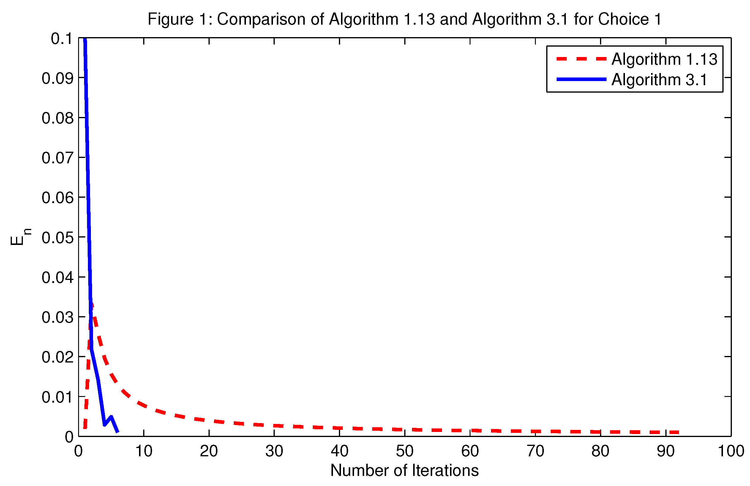
Remark 1.

It is noted that the condition

$$\begin{array}{c}\hfill {\displaystyle \underset{n\to \infty }{\lim }({\lambda }_n-{\lambda }_{n+1})=0}\end{array}$$

is removed from Theorem TTT of Takahashi et al. [12].

Remark 2.

[17] We remark here that the conditions (C4) is easily implemented in numerical computation since the valued of $\parallel x_n-x_{n-1}\parallel$ is known before choosing ${\theta }_n$. Indeed, the parameter ${\theta }_n$ can be chosen such that $0\le {\theta }_n\le {\overline{\theta }}_n$, where

$${\overline{\theta }}_n=\left\{\begin{array}{c}\min \left\{\frac{{\omega }_n}{\parallel x_n-x_{n-1}\parallel },\theta \right\}if{x}_n\ne x_{n-1},\hfill \\ \theta otherwise,\hfill \end{array}\right.$$

where $\left\{{\omega }_n\right\}$ is a positive sequence such that ${\omega }_n=o\left({\alpha }_n\right)$.

4. Weak Convergence Theorem

In this section, we prove the weak convergence theorem.

Theorem 3.

Let C be a nonempty, closed, and convex subset of a real Hilbert space H. Let A be an α-inverse strongly monotone mapping of H into itself and let B be a maximal monotone operator on H such that the domain of B is included in C. Let $J_{\lambda }={(I+\lambda B)}^{-1}$ be the resolvent of B for $\lambda >0$ and let S be a nonexpansive mapping of C into itself such that $F\left(S\right)\cap {(A+B)}^{-1}0\ne \varnothing$. Let $x_0,x_1\in C$ and let $\left\{x_n\right\}\subset C$ be a sequence generated by

$$\begin{array}{ccc}\hfill y_n& =& x_n+{\theta }_n(x_n-x_{n-1}),\hfill \\ \hfill x_{n+1}& =& {\beta }_n{x}_n+(1-{\beta }_n)S\left(J_{{\lambda }_n}(y_n-{\lambda }_{n}A{y}_n)\right)\hfill \end{array}$$

(39)

for all $n\in \mathbb{N}$, where $\left\{{\lambda }_n\right\}\subset (0,2\alpha ),\left\{{\beta }_n\right\}\subset (0,1)$ and $\left\{{\theta }_n\right\}\subset [0,\theta ]$, where $\theta \in [0,1)$ satisfy

(C1) 

${\displaystyle \underset{n\to \infty }{\mathrm{lim\; inf}} {\beta }_n(1-{\beta }_n)>0}$;

(C2) 

${\displaystyle 0<\underset{n\to \infty }{\mathrm{lim\; inf}} {\lambda }_n\le \underset{n\to \infty }{\mathrm{lim\; sup}} {\lambda }_n<2\alpha }$;

(C3) 

${\displaystyle \sum _{n=1}^{\infty }{\theta }_n{\parallel x_n-x_{n-1}\parallel }^2<\infty }$.

Then $\left\{x_n\right\}$ converges weakly to a point of $F\left(S\right)\cap {(A+B)}^{-1}0$.

Proof. 

Let $z\in F\left(S\right)\cap {(A+B)}^{-1}0$ and $w_n=J_{{\lambda }_n}(y_n-{\lambda }_{n}A{y}_n)\forall n\ge 1$. Then $z=J_{{\lambda }_n}(z-{\lambda }_{n}Az)$. From Theorem 2 we have

$$\begin{array}{c}\hfill \parallel x_{n+1}{-z\parallel }^2\le {\beta }_n\parallel x_n{-z\parallel }^2+(1-{\beta }_n)\parallel w_n{-z\parallel }^2-{\beta }_n(1-{\beta }_n){\parallel x_n-S{w}_n\parallel }^2,\end{array}$$

(40)

$$\begin{array}{ccc}\hfill \parallel w_n{-z\parallel }^2& =& \parallel y_n{-z\parallel }^2-{\lambda }_n(2\alpha -{\lambda }_n){\parallel A{y}_n-Az\parallel }^2\hfill \\ & & -\parallel y_n-{\lambda }_n(A{y}_n-Az)-J_{{\lambda }_n}(y_n-{\lambda }_{n}A{y}_n){\parallel }^2\hfill \end{array}$$

(41)

and

$$\begin{array}{c}\hfill \parallel y_n{-z\parallel }^2\le (1+{\theta }_n)\parallel x_n{-z\parallel }^2+2{\theta }_n\parallel x_n-x_{n-1}{\parallel }^2-{\theta }_n{\parallel x_{n-1}-z\parallel }^2.\end{array}$$

(42)

Combining (42) and (41), we obtain

$$\begin{array}{ccc}\hfill \parallel w_n{-z\parallel }^2& \le & (1+{\theta }_n)\parallel x_n{-z\parallel }^2+2{\theta }_n\parallel x_n-x_{n-1}{\parallel }^2-{\theta }_n{\parallel x_{n-1}-z\parallel }^2\hfill \\ & & -{\lambda }_n(2\alpha -{\lambda }_n)\parallel A{y}_n{-Az\parallel }^2-{\parallel y_n-{\lambda }_n(A{y}_n-Az)-J_{{\lambda }_n}(y_n-{\lambda }_{n}A{y}_n)\parallel }^2.\hfill \end{array}$$

(43)

Combining (40) and (43), we also have

$$\begin{array}{ccc}\hfill \parallel x_{n+1}{-z\parallel }^2& \le & {\beta }_n\parallel x_n{-z\parallel }^2+(1-{\beta }_n)[(1+{\theta }_n)\parallel x_n{-z\parallel }^2+2{\theta }_n{\parallel x_n-x_{n-1}\parallel }^2\hfill \\ & & -{\theta }_n\parallel x_{n-1}{-z\parallel }^2-{\lambda }_n(2\alpha -{\lambda }_n){\parallel A{y}_n-Az\parallel }^2\hfill \\ & & -\parallel y_n-{\lambda }_n(A{y}_n-Az)-J_{{\lambda }_n}(y_n-{\lambda }_{n}A{y}_n)\parallel ]-{\beta }_n(1-{\beta }_n){\parallel x_n-S{w}_n\parallel }^2\hfill \\ & =& {\beta }_n\parallel x_n{-z\parallel }^2+(1-{\beta }_n)(1+{\theta }_n)\parallel x_n{-z\parallel }^2+2{\theta }_n(1-{\beta }_n){\parallel x_n-x_{n-1}\parallel }^2\hfill \\ & & -{\theta }_n(1-{\beta }_n)\parallel x_{n-1}{-z\parallel }^2-{\lambda }_n(2\alpha -{\lambda }_n)(1-{\beta }_n){\parallel A{y}_n-Az\parallel }^2\hfill \\ & & -(1-{\beta }_n){\parallel y_n-{\lambda }_n(A{y}_n-Az)-J_{{\lambda }_n}(y_n-{\lambda }_{n}A{y}_n)\parallel }^2\hfill \\ & & -{\beta }_n(1-{\beta }_n){\parallel x_n-S{w}_n\parallel }^2\hfill \\ & \le & \parallel x_n{-z\parallel }^2+{\theta }_n(1-{\beta }_n){\parallel x_n-z\parallel }^2\hfill \\ & & +2{\theta }_n(1-{\beta }_n)\parallel x_n-x_{n-1}{\parallel }^2-{\theta }_n(1-{\beta }_n){\parallel x_{n-1}-z\parallel }^2.\hfill \end{array}$$

(44)

This shows that

$$\begin{array}{ccc}\hfill \parallel x_{n-1}{-z\parallel }^2-{\parallel x_n-z\parallel }^2& \le & {\theta }_n(1-{\beta }_n)[\parallel x_n{-z\parallel }^2-\parallel x_{n-1}-z{\parallel }^2]\hfill \\ & & +2{\theta }_n(1-{\beta }_n){\parallel x_n-x_{n-1}\parallel }^2.\hfill \end{array}$$

By Lemma 4, we have $\parallel x_n{-z\parallel }^2$ converges. Thus, ${\displaystyle \underset{n\to \infty }{\lim }{\parallel x_n-z\parallel }^2}$ exists. So, by (44) we have

$$\begin{array}{ccc}\hfill {\lambda }_n(2\alpha -{\lambda }_n)(1-{\beta }_n){\parallel A{y}_n-Az\parallel }^2& \le & {\theta }_n(1-{\beta }_n)[\parallel x_n{-z\parallel }^2-\parallel x_{n-1}-z{\parallel }^2]\hfill \\ & & +2{\theta }_n(1-{\beta }_n)\parallel x_n-x_{n-1}{\parallel }^2+\parallel x_n{-z\parallel }^2-{\parallel x_{n+1}-z\parallel }^2\hfill \\ & \to & 0,asn\to \infty .\hfill \end{array}$$

We also have

$$\begin{array}{ccc}\hfill (1-{\beta }_n){\parallel y_n-{\lambda }_n(A{y}_n-Az)-J_{{\lambda }_n}(y_n-{\lambda }_{n}A{y}_n)\parallel }^2& \le & {\theta }_n(1-{\beta }_n)[\parallel x_n{-z\parallel }^2-\parallel x_{n-1}-z{\parallel }^2]\hfill \\ & & +2{\theta }_n(1-{\beta }_n)\parallel x_n-x_{n-1}{\parallel }^2+{\parallel x_n-z\parallel }^2\hfill \\ & & -\parallel x_{n+1}{-z\parallel }^2\hfill \\ & \to & 0,asn\to \infty .\hfill \end{array}$$

Moreover, we obtain

$$\begin{array}{ccc}\hfill {\beta }_n(1-{\beta }_n){\parallel x_n-S{w}_n\parallel }^2& \le & {\theta }_n(1-{\beta }_n)[\parallel x_n{-z\parallel }^2-\parallel x_{n-1}-z{\parallel }^2]\hfill \\ & & +2{\theta }_n(1-{\beta }_n)\parallel x_n-x_{n-1}{\parallel }^2+\parallel x_n{-z\parallel }^2-{\parallel x_{n+1}-z\parallel }^2\hfill \\ & \to & 0,asn\to \infty .\hfill \end{array}$$

It follows that

$$\parallel A{y}_n-Az\parallel \to 0,\parallel y_n-{\lambda }_n(A{y}_n-Az)-J_{{\lambda }_n}(y_n-{\lambda }_{n}A{y}_n)\parallel \to 0 \mathrm{and} \parallel x_n-S{w}_n\parallel \to 0$$

.

By a similar proof as in Theorem 2, we can show that if there exists a subsequence $\left\{x_{n_k}\right\}$ of $\left\{x_n\right\}$, such that $x_{n_k}\rightharpoonup x^{\ast }$, then $x^{\ast }\in F\left(S\right)\cap {(A+B)}^{-1}0$. By Lemma 3, we conclude that $\left\{x_n\right\}$ weakly converges to a point in $F\left(S\right)\cap {(A+B)}^{-1}0$. We thus complete the proof. □

Remark 3.

[18] We remark here that the conditions (C3) is easily implemented in numerical computation. Indeed, once $x_n$ and $x_{n-1}$ are given, it is just sufficient to compute the update $x_{n+1}$ with (39) by choosing ${\theta }_n$ such that $0\le {\theta }_n\le {\overline{\theta }}_n$, where

$${\overline{\theta }}_n=\left\{\begin{array}{c}\min \left\{\frac{{\epsilon }_n}{\parallel x_n-x_{n-1}{\parallel }^2},\theta \right\}if{x}_n\ne x_{n-1},\hfill \\ \theta otherwise,\hfill \end{array}\right.$$

where $\left\{{\epsilon }_n\right\}\subset [0,\infty )$ is such that ${\displaystyle \sum _{n=1}^{\infty }{\epsilon }_n<\infty }$.

5. Numerical Examples

In this section, we give some numerical experiments to show the efficiency and the comparison with other methods.

Example 1.

Solve the following minimization problem:

$$\begin{array}{c}\hfill {\displaystyle \underset{x\in {\mathbb{R}}^3}{\min }\parallel x{\parallel }_2^2+(3,5,-1)x+9+\parallel x{\parallel }_1,}\end{array}$$

where $x=(y_1,y_2,y_3)\in {\mathbb{R}}^3$ and the fixed-point problem of $S:{\mathbb{R}}^3\to {\mathbb{R}}^3$ defined by

$$\begin{array}{c}\hfill S\left(x\right)=(-2-y_1,-4-y_2,-y_3).\end{array}$$

For each $x\in {\mathbb{R}}^3$, we set $F\left(x\right)=\parallel x{\parallel }_2^2+(3,5,-1)x+9$ and $G\left(x\right)=\parallel x{\parallel }_1$. Put $A=\nabla F$ and $B=\partial G$ in Theorem 2. We can check that F is convex and differentiable on ${\mathbb{R}}^3$ with 2-Lipschitz continuous gradient. Moreover, G is convex and lower semi-continuous but not differentiable on ${\mathbb{R}}^3$. We know that for $r>0$

$$\begin{array}{c}\hfill {(I+rB)}^{-1}\left(x\right)=(max\{\mid y_1\mid -r,0\}sign\left(y_1\right),max\{\mid y_2\mid -r,0\}sign\left(y_2\right),max\{\mid y_3\mid -r,0\}sign\left(y_3\right)).\end{array}$$

(45)

We choose ${\alpha }_n=\frac{1}{100n+1},$${\beta }_n=\frac{3n}{5n+1},$${\lambda }_n=0.0001$ for all $n\in \mathbb{N}$ and $\theta =0.5.$ For each $n\in \mathbb{N},$ let ${\omega }_n=\frac{1}{{(n+1)}^3}$ and define ${\theta }_n=\overline{{\theta }_n}$ as in Remark 2. The stopping criterion is defined by

$$\begin{array}{c}\hfill E_n=\parallel x_n-J_{{\lambda }_n}(I-\nabla F)x_n\parallel +\parallel x_n-S{x}_n\parallel <{10}^{-3}.\end{array}$$

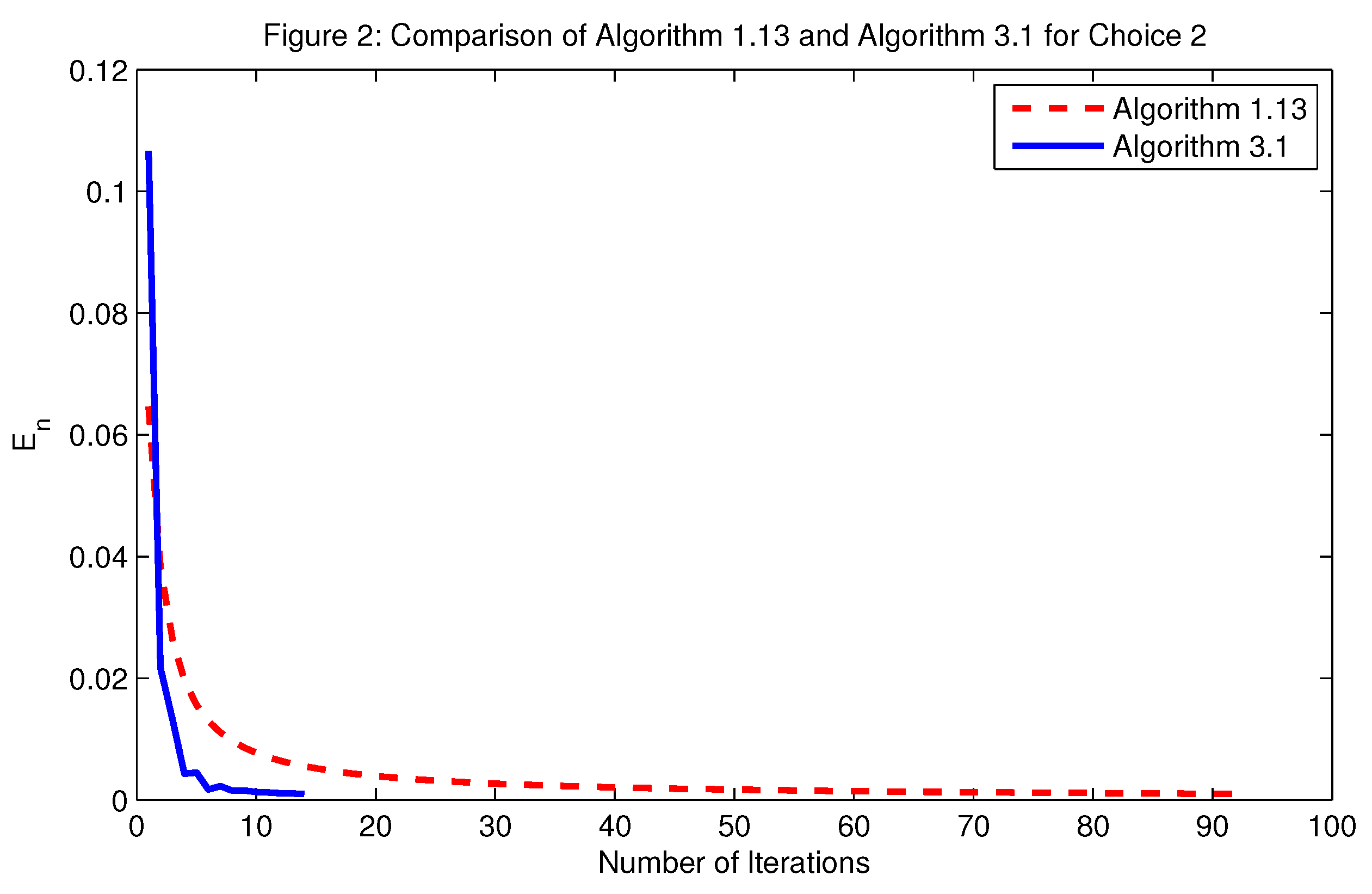
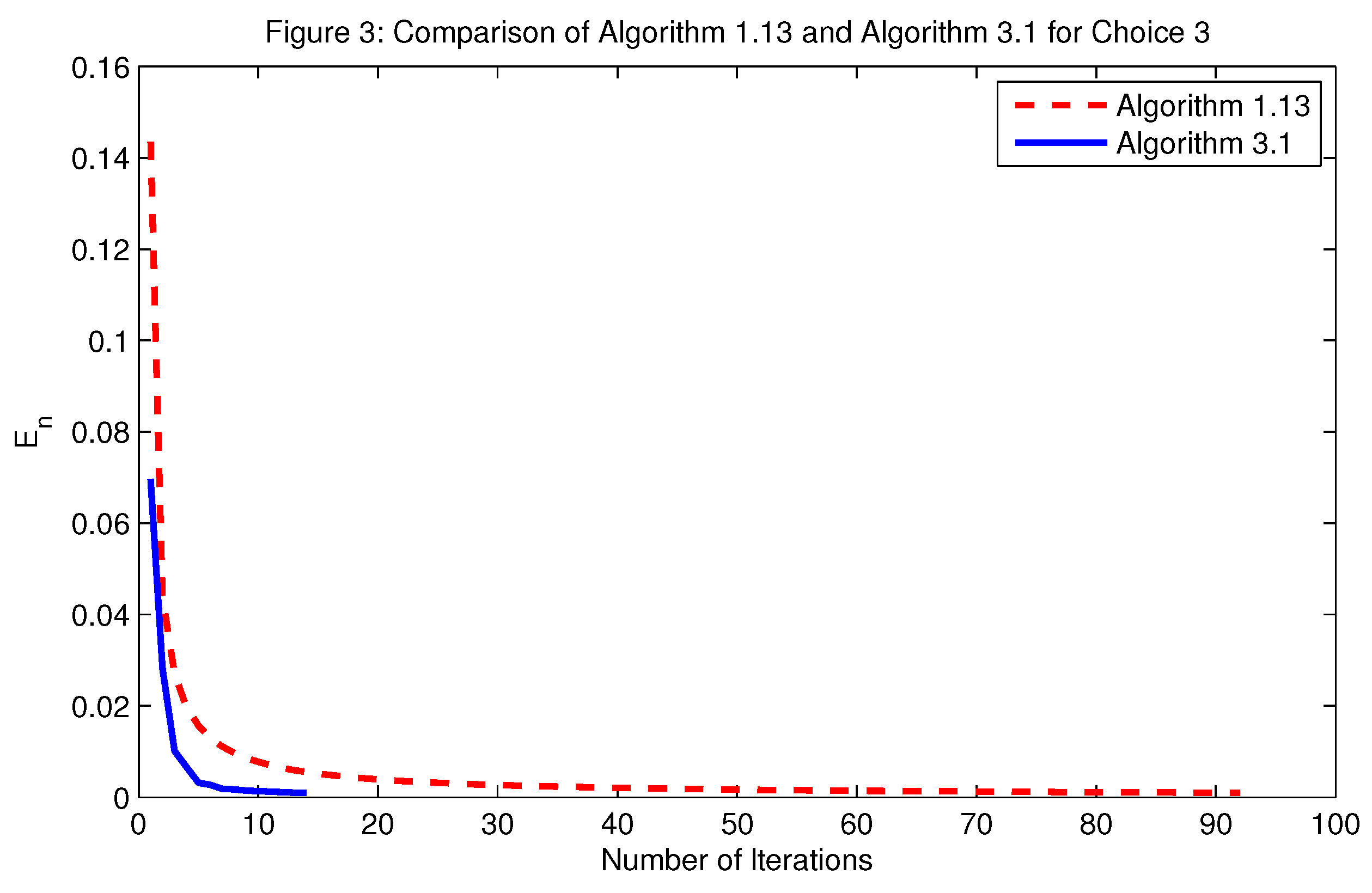
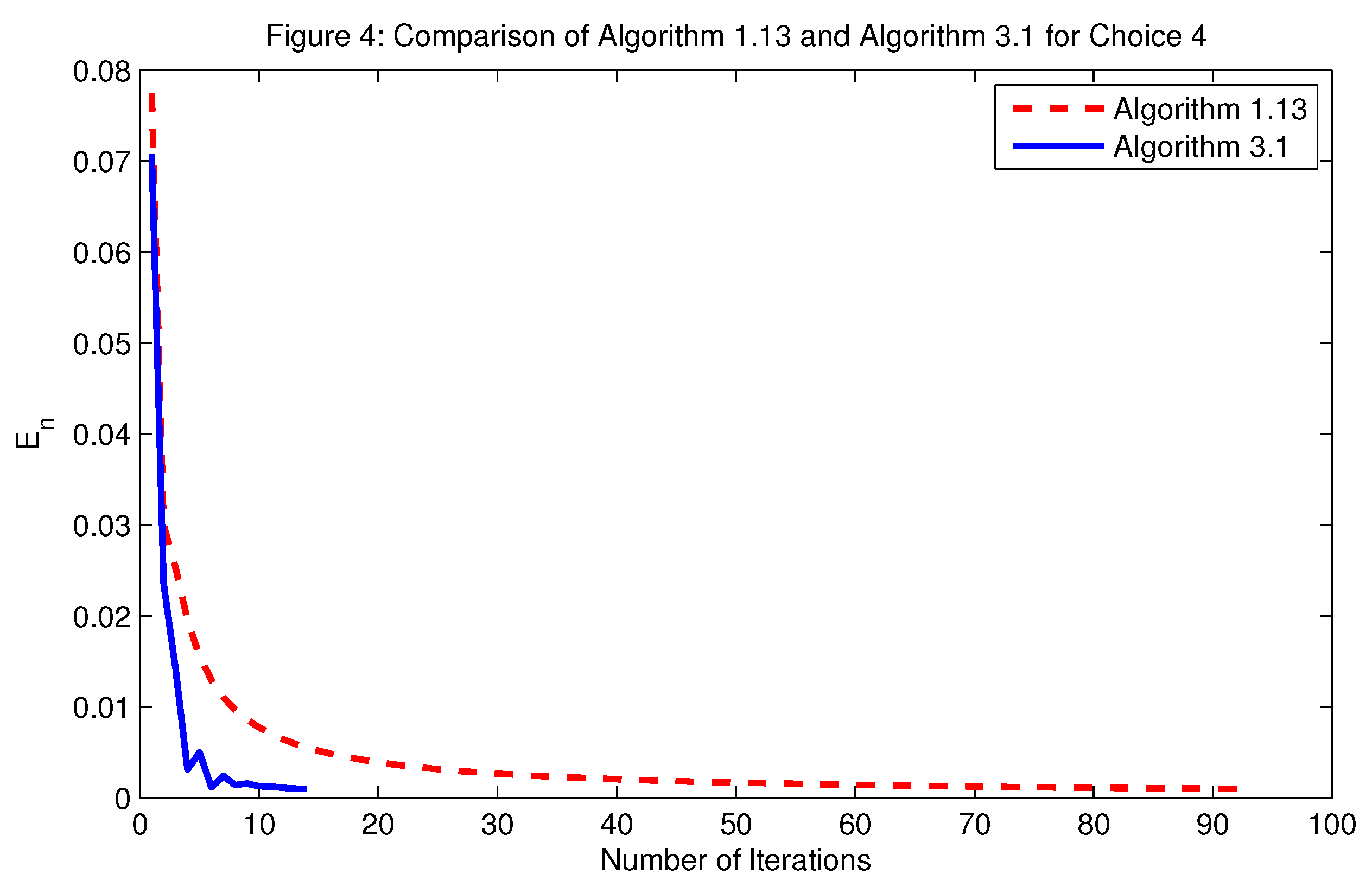
We now study the effect (in terms of convergence and the CPU time) and consider different choices of $x_0$ and $x_1$ as following, see

Table 1. Using Equations (13) and (25) with different choices of $x_0$ and $x_1$.

			Equation (13)	Equation (25)
Choice 1	$x_0=(1,2,-1)$	No. of Iter.	92	6
	$x_1=(1,5,1)$	CPU (Time)	$0.045106$	$0.016301$
Choice 2	$x_0=(0,-2,2)$	No. of Iter.	92	14
	$x_1=(2,0,-3)$	CPU (Time)	$0.039239$	$0.014759$
Choice 3	$x_0=(-5,4,6)$	No. of Iter.	92	14
	$x_1=(3,-5,-9)$	CPU (Time)	$0.064943$	$0.010813$
Choice 4	$x_0=(1,2,3)$	No. of Iter.	92	14
	$x_1=(8,7,3)$	CPU (Time)	$0.066736$	$0.047984$

.

• Choice 1: $x_0=(1,2,-1)$ and $x_1=(1,5,1)$;
• Choice 2: $x_0=(0,-2,2)$ and $x_1=(2,0,-3)$;
• Choice 3: $x_0=(-5,4,6)$ and $x_1=(3,-5,-9)$;
• Choice 4: $x_0=(1,2,3)$ and $x_1=(8,7,3)$.

The error plotting of Equations (13) and (25) for each choice is shown in Figure 1, Figure 2, Figure 3 and Figure 4, respectively.

References

1. Xu, H.K. A regularization method for the proximal point algorithm. J. Glob. Optim. 2006, 36, 115–125. [Google Scholar] [CrossRef]
2. Kamimura, S.; Takahashi, W. Approximating solutions of maximal monotone operators in Hilbert spaces. J. Approx. Theory 2000, 106, 226–240. [Google Scholar] [CrossRef]
3. Boikanyo, O.A.; Morosanu, G. A proximal point algorithm converging strongly for general errors. Optim. Lett. 2010, 4, 635–641. [Google Scholar] [CrossRef]
4. Boikanyo, O.A.; Morosanu, G. Strong convergence of a proximal point algorithm with bounded errorsequence. Optim. Lett. 2013, 7, 415–420. [Google Scholar] [CrossRef]
5. Marino, G.; Xu, H.K. Convergence of generalized proximal point algorithm. Commun. Pure Appl. Anal. 2004, 3, 791–808. [Google Scholar]
6. Yao, Y.; Noor, M.A. On convergence criteria of generalized proximal point algorithms. J. Comput. Appl. Math. 2008, 217, 46–55. [Google Scholar] [CrossRef]
7. Wang, F.; Cui, H. On the contraction-proximal point algorithms with multi-parameters. J. Glob. Optim. 2012, 54, 485–491. [Google Scholar] [CrossRef]
8. Takahashi, W. Viscosity approximation methods for resolvents of accretive operators in Banach spaces. J. Fixed Point Theory Appl. 2007, 1, 135–147. [Google Scholar] [CrossRef]
9. Combettes, P.L. Iterative construction of the resolvent of a sum of maximal monotone operators. J. Convex Anal. 2009, 16, 727–748. [Google Scholar]
10. Lopez, G.; Martín-Márquez, V.; Wang, F.; Xu, H.K. Forward-Backward splitting methods for accretive operators in Banach spaces. Abstr. Appl. Anal. 2012, 2012, 109–236. [Google Scholar] [CrossRef]
11. Lehdili, N.; Moudafi, A. Combining the proximal algorithm and Tikhonov regularization. Optimization 1996, 37, 239–252. [Google Scholar] [CrossRef]
12. Takahashi, S.; Takahashi, W.; Toyoda, M. Strong convergence theorems for maximal monotone operators with nonlinear mappings in Hilbert spaces. J. Optim. Theory Appl. 2010, 147, 27–41. [Google Scholar] [CrossRef]
13. Takahashi, W.; Tamura, T. Convergence theorems for a pair of nonexpansive mappings. J. Convex Anal. 1998, 5, 45–56. [Google Scholar]
14. Halpern, B. Fixed points of nonexpanding maps. Bull. Am. Math. Soc. 1967, 73, 957–961. [Google Scholar] [CrossRef]
15. Dong, Q.L.; Cho, Y.J.; Zhong, L.L.; Rassias, T.M. Inertial projection and contraction algorithms for variational inequalities. J. Glob. Optim. 2018, 70, 687–704. [Google Scholar] [CrossRef]
16. Dong, Q.L.; Yuan, H.B.; Cho, Y.J.; Rassias, T.M. Modified inertial Mann algorithm and inertial CQ-algorithm for nonexpansive mappings. Optim. Lett. 2018, 12, 87–102. [Google Scholar] [CrossRef]
17. Suantai, S.; Pholasa, N.; Cholamjiak, P. The modified inertial relaxed CQ algorithm for solving the split feasibility problems. J. Ind. Manag. Optim. 2018, 14, 1595–1615. [Google Scholar] [CrossRef]
18. Maingé, P.E. Convergence theorems for inertial KM-type algorithms. J. Comput. Appl. Math. 2008, 219, 223–236. [Google Scholar] [CrossRef]
Figure 1. Comparison of Equations (13) and (25) for each choice 1.
Mathematics 07 00167 g001
Figure 2. Comparison of Equations (13) and (25) for each choice 2.
Mathematics 07 00167 g002
Figure 3. Comparison of Equations (13) and (25) for each choice 3.
Mathematics 07 00167 g003
Figure 4. Comparison of Equations (13) and (25) for each choice 4.
Mathematics 07 00167 g004