Article

Analysis of General Humoral Immunity HIV Dynamics Model with HAART and Distributed Delays

1
Department of Mathematics, Faculty of Science, King Abdulaziz University, P.O. Box 80203, Jeddah 21589, Saudi Arabia
2
Department of Mathematics, Faculty of Science, Al-Azhar University, Assiut 71524, Egypt
3
Department of Mathematics, Faculty of Science, Sohag University, Sohag 82524, Egypt
*
Author to whom correspondence should be addressed.
Mathematics 2019, 7(2), 157; https://doi.org/10.3390/math7020157
Submission received: 2 December 2018 / Revised: 27 January 2019 / Accepted: 31 January 2019 / Published: 9 February 2019

Abstract

:
This paper deals with the study of an HIV dynamics model with two target cells, macrophages and CD4 + T cells and three categories of infected cells, short-lived, long-lived and latent in order to get better insights into HIV infection within the body. The model incorporates therapeutic modalities such as reverse transcriptase inhibitors (RTIs) and protease inhibitors (PIs). The model is incorporated with distributed time delays to characterize the time between an HIV contact of an uninfected target cell and the creation of mature HIV. The effect of antibody on HIV infection is analyzed. The production and removal rates of the ten compartments of the model are given by general nonlinear functions which satisfy reasonable conditions. Nonnegativity and ultimately boundedness of the solutions are proven. Using the Lyapunov method, the global stability of the equilibria of the model is proven. Numerical simulations of the system are provided to confirm the theoretical results. We have shown that the antibodies can play a significant role in controlling the HIV infection, but it cannot clear the HIV particles from the plasma. Moreover, we have demonstrated that the intracellular time delay plays a similar role as the Highly Active Antiretroviral Therapies (HAAT) drugs in eliminating the HIV particles.

1. Introduction

Modeling the HIV dynamics has received considerable attention from mathematicians during the recent decades [1,2,3,4,5,6,7,8,9,10,11,12,13,14,15,16,17,18,19,20,21,22]. The first HIV dynamics model is proposed by Nowak and Bangham [1] as:
s ˙ t = ρ δ s t λ ¯ s t p t ,
y ˙ t = λ ¯ s t p t η y t ,
p ˙ t = N ¯ η y t g p ( t ) ,
where s, y and p are the concentrations of the CD4 + T cells, infected cells and HIV particles; ρ , δ and λ ¯ represent the production, death and infection rates of the uninfected CD4 + T cells, respectively; η and g are the death rate constants of the infected cells and free HIV, respectively; N ¯ is the average number of HIV particles generated in the lifetime of the infected cells. A class of latently infected cells has been modeled in the HIV dynamics in [23,24,25,26]. Elaiw et al. [27] have extended model (1)–(3) by considering distributed time delays, B cells (x), and three categories of infected cells, short-lived (y), long-lived (u) and latent (w) as:
s ˙ = π ( s t ) λ Υ ( s t , p t ) ,
w ˙ = λ 1 0 h 1 f 1 τ e μ 1 τ Υ ( s t τ , p t τ ) d τ ( α + β ) ψ 1 ( w t ) ,
y ˙ = λ 2 0 h 2 f 2 τ e μ 2 τ Υ ( s t τ , p t τ ) d τ + α ψ 1 ( w t ) η ψ 2 ( y t ) ,
u ˙ = λ 3 0 h 3 f 3 τ e μ 3 τ Υ ( s t τ , p t τ ) d τ ν ψ 3 ( u t ) ,
p ˙ = N η ψ 2 ( y t ) + M ν ψ 3 ( u t ) g ψ 4 ( p t ) μ ψ 4 ( p t ) ψ 5 ( x t ) ,
x ˙ = r ψ 4 ( p t ) ψ 5 ( x t ) ω ψ 5 ( x t ) ,
where f i τ e μ i τ over the time interval 0 , h i , i = 1 , 2 , 3 represents the probabilities that uninfected cells contacted by HIV at time t τ survived τ time units and become infected at time t; Υ , π , ψ j , j = 1 , , 5 are general nonlinear functions. The probability distribution function f i τ satisfies f i τ > 0 and
0 h i f i τ d τ = 1 , 0 h i f i η e υ η d η < , i = 1 , 2 , 3 ,
where υ > 0 . Let us denote Θ i ( τ ) = f i ( τ ) e μ i τ and F i = 0 h i Θ i ( τ ) d τ , thus 0 < F i 1 , i = 1 , 2 , 3 .
Model (4)–(9) assumes that the HIV infects one category of target cells, CD4 + T cells. However, Perleson et al. have observed that after the rapid first phase of decay during the initial 1–2 weeks of an antiretroviral treatment, plasma virus levels declined at a considerably slower rate [28]. This second phase of viral decay was attributed to the turnover of infected macrophages. Therefore, the HIV model with two categories of target cells, CD4 + T cells and macrophages is more accurate than that model with only one category target cells, CD4 + T cells. As a result, more accurate drug efficacy can be determined when using the HIV model with two classes of target cells. Recently, many efforts have been devoted to the analysis of various mathematical models of HIV dynamics with two categories of target cells (see, e.g., [29,30,31,32,33,34,35,36,37]). However, in these papers, the production and removal rates of the HIV particles and cells are given by linear functions; moreover, only one or two classes of infected cells are considered.
The aim of the present paper is to propose and analyze an HIV dynamics model which extends model (4)–(9) and describes the dynamics of HIV with two categories of target cells, CD4 + T cells and macrophages. We study the basic and global properties of the model. Using Lyapunov function and LaSalle’s invariance principle, we have established the global asymptotic stability of the three equilibria of the model. We have shown that the antibodies can reduce the HIV level, but they cannot clear the HIV particles completely. The effect of HAART drugs and intracellular time delays in stabilizing the HIV dynamics system around the infection-free equilibrium are shown. The importance of considering the second class of target cells (macrophages) in the HIV dynamics is also shown.
The rest of the paper is organized as follows: in Section 2, we present the HIV model and study its basic properties. In Section 3, the global stability of three equilibria is established. In Section 4, we offer some numerical simulations to confirm our analytical results. The paper ends with some conclusions and discussion in Section 5.

2. Mathematical Model

We propose the following model:
s ˙ i = π i ( s i t ) λ i Υ i ( s i t , p t ) ,
w ˙ i = λ 1 i 0 h 1 i f 1 i τ e μ 1 i τ Υ i ( s i t τ , p t τ ) d τ ( α i + β i ) ψ 1 i ( w i t ) ,
y ˙ i = λ 2 i 0 h 2 i f 2 i τ e μ 2 i τ Υ i ( s i t τ , p t τ ) d τ + α i ψ 1 i ( w i t ) η i ψ 2 i ( y i t ) ,
u ˙ i = λ 3 i 0 h 3 i f 3 i τ e μ 3 i τ Υ i ( s i t τ , p t τ ) d τ ν i ψ 3 i ( u i t ) ,
p ˙ = i = 1 2 N i η i 0 h 4 i f 4 i τ e μ 4 i τ ψ 2 i ( y i t τ ) d τ + M i ν i 0 h 5 i f 5 i τ e μ 5 i τ ψ 3 i ( u i t τ ) d τ g ψ 41 ( p t ) μ ψ 41 ( p t ) ψ 42 ( x t ) ,
x ˙ = r ψ 41 ( p t ) ψ 42 ( x t ) ω ψ 42 ( x t ) ,
where i = 1 for the CD4 + T cells and i = 2 for the macrophages. We have λ m 1 = ( 1 ε 1 ) λ ¯ m 1 , λ m 2 = ( 1 f ε 1 ) λ ¯ m 2 , m = 1 , 2 , 3 , N 1 = ( 1 ε 2 ) N ¯ 1 , M 1 = ( 1 ε 2 ) M ¯ 1 , N 2 = ( 1 h ε 2 ) N ¯ 2 , M 2 = ( 1 h ε 2 ) M ¯ 2 , λ i = λ 1 i + λ 2 i + λ 3 i , and f , h ( 0 , 1 ) . Let f j i τ e μ j i τ over the time interval 0 , h j i , j = 1 , , 5 , i = 1 , 2 , are the probabilities that uninfected target cells contacted by HIV at time t τ survived τ time units and became infected at time t. Denote Θ j i ( τ ) = f j i ( τ ) e μ j i τ and F j i = 0 h j i Θ j i ( τ ) d τ ; thus 0 < F j i 1 , j = 1 , , 5 , i = 1 , 2 . We assume that:
Hypothesis 1 (H1).
(i) There exists s i 0 such that π i ( s i 0 ) = 0 , π i ( s i ) > 0 for s i [ 0 , s i 0 ) , (ii) π i ( s i ) < 0 for s i > 0 ; (iii) there are b i > 0 and b ¯ i > 0 such that π i ( s i ) b i b ¯ i s i for s i 0 .
Hypothesis 2 (H2).
(i) Υ i ( s i , p ) > 0 and Υ i ( 0 , p ) = Υ i ( s i , 0 ) = 0 for s i , p > 0 , (ii) Υ i ( x i , p ) s i > 0 , Υ i ( s i , p ) p > 0 and, Υ i ( s i , 0 ) p > 0 for all s i , p > 0 , (iii) d d s i Υ i ( s i , 0 ) p > 0 for s i > 0 .
Hypothesis 3 (H3).
(i) ψ j i ( η ) > 0 for η > 0 , ψ j i ( 0 ) = 0 , j = 1 , , 4 , i = 1 , 2 , (ii) ψ j i ( η ) > 0 , ψ 42 ( η ) > 0 for η > 0 , j = 1 , 2 , 3 , i = 1 , 2 , ψ 41 ( η ) > 0 , for η 0 ; (iii) there are α j i > 0 , j = 1 , , 4 , i = 1 , 2 , such that ψ j i ( η ) α j i η for η 0 .
Hypothesis 4 (H4).
Υ i ( s i , p ) ψ 41 ( p ) is decreasing function w.r.t.p, for p > 0 .
Remark 1.
From H1–H4, we have
Υ i ( s i , p ) Υ i ( s i , p * ) Υ i ( s i , p ) ψ 41 p Υ i ( s i , p * ) ψ 41 p * 0 ,
which gives
1 Υ i ( s i , p * ) Υ i ( s i , p ) Υ i ( s i , p ) Υ i ( s i , p * ) ψ 41 p ψ 41 p * 0 .
We consider systems (10)–(15) with the initial conditions:
s 1 t = φ 1 θ , s 2 t = φ 2 θ , w 1 t = φ 3 θ , w 2 t = φ 4 θ , y 1 t = φ 5 θ , y 2 t = φ 6 θ , u 1 t = φ 7 θ , u 2 t = φ 8 θ , p t = φ 9 θ , x t = φ 10 θ , φ j θ 0 , θ ς , 0 , j = 1 , , 10 ,
where ς = max h 11 , h 12 , h 21 , h 22 , h 31 , h 32 , h 41 , h 42 , h 51 , h 52 and denoted by C is the Banach space of continuous functions mapping the interval ς , 0 into R 0 and φ 1 θ , , φ 10 θ C ς , 0 , R 0 10 . According to [38], there exists a unique solution for system (10)–(15) with initial (16).

2.1. Properties of Solutions

Lemma 1.
Suppose that H1–H3 hold, then the solutions of system (10)–(15) are non-negative and ultimately bounded.
The proof Lemma 1 is given in Appendix A.
Lemma 1 shows that
Ω = ( s 1 , s 2 , w 1 , w 2 , y 1 , y 2 , u 1 , u 2 , p , x ) C 10 : s i M 1 i , w i M 1 i , y i M 2 i , u i M 3 i , p M 41 , x M 42
is positively invariant with respect to system (10)–(15).

2.2. Equilibria

The basic reproduction number R 0 of system (10)–(15) is given by:
R 0 = i = 1 2 γ i ψ 41 ( 0 ) Υ i ( s i 0 , 0 ) p .
The equilibria of system (10)–(15) satisfy the following equations:
0 = π i ( s i ) λ i Υ i ( s i , p ) ,
0 = λ 1 i F 1 i Υ i ( s i , p ) ( α i + β i ) ψ 1 i ( w i ) ,
0 = λ 2 i F 2 i Υ i ( s i , p ) + α i ψ 1 i ( w i ) η i ψ 2 i ( y i ) ,
0 = λ 3 i F 3 i Υ i ( s i , p ) ν i ψ 3 i ( u i ) ,
0 = i = 1 2 N i η i F 4 i ψ 2 i ( y i ) + M i ν i F 5 i ψ 3 i ( u i ) g ψ 41 ( p ) μ ψ 41 ( p ) ψ 42 ( x ) ,
0 = r ψ 41 ( p ) ψ 42 ( x ) ω ψ 42 ( x ) .
From Equation (22), we have x = 0 or p = ψ 41 1 ( ω / r ) . Let us define
Λ 1 i ( s i ) = ψ 1 i 1 λ 1 i F 1 i λ i ( α i + β i ) π i ( s i ) , Λ 2 i ( s i ) = ψ 2 i 1 α i λ 1 i F 1 i + ( α i + β i ) λ 2 i F 2 i λ i η i ( α i + β i ) π i ( s i ) , Λ 3 i ( s i ) = ψ 3 i 1 λ 3 i F 3 i λ i ν i π i ( s i ) , Λ 4 ( s i ) = ψ 41 1 i = 1 2 γ i λ i π i ( s i ) ,
where γ i = i = 1 2 N i F 4 i ( α i λ 1 i F 1 i + ( α i + β i ) λ 2 i F 2 i ) + M i F 3 i F 5 i λ 3 i ( α i + β i ) g ( α i + β i ) . It follows from Equations (17)–(21) that:
w i = Λ 1 i ( s i ) , y i = Λ 2 i ( s i ) , u i = Λ 3 i ( s i ) , p = Λ 4 ( s i ) .
Obviously, Λ 1 i ( s i ) , Λ 2 i ( s i ) , Λ 3 i ( s i ) , Λ 4 ( s i ) > 0 for s i [ 0 , s i 0 ) and Λ 1 i ( s i 0 ) = Λ 2 i ( s i 0 ) = Λ 3 i ( s i 0 ) = Λ 4 ( s i 0 ) = 0 , i = 1 , 2 . From Equations (17), (23), and (24), we obtain
i = 1 2 γ i Υ i ( s i , Λ 4 ( s i ) ) ψ 41 ( Λ 4 ( s i ) ) = 0 .
Equation (25) has two possible solutions, Λ 4 = 0 and Λ 4 0 . The solution Λ 4 = 0 implies s i = s i 0 which gives the infection-free equilibrium Π 0 ( s 1 0 , s 2 0 , 0 , 0 , 0 , 0 , 0 , 0 , 0 , 0 ) . The other solution Λ 4 0 admits an antibody-inactivated infection equilibrium Π 1 ( s ˜ 1 , s ˜ 2 , w ˜ 1 , w ˜ 2 , y ˜ 1 , y ˜ 2 , u ˜ 1 , u ˜ 2 , p ˜ , 0 ) , where
π i ( s ˜ i ) = λ i Υ i ( s ˜ i , p ˜ ) , λ 1 i F 1 i Υ i ( s ˜ i , p ˜ ) = ( α i + β i ) ψ 1 i ( w ˜ i ) , η i ψ 2 i ( y ˜ i ) = λ 2 i F 2 i Υ i ( s ˜ i , p ˜ ) + α i ψ 1 i ( w ˜ i ) , ν i ψ 3 i ( u ˜ i ) = λ 3 i F 3 i Υ i ( s ˜ i , p ˜ ) , g ψ 41 ( p ˜ ) = i = 1 2 N i η i F 4 i ψ 2 i ( y ˜ i ) + M i ν i F 5 i ψ 3 i ( u ˜ i ) .
Now, we consider the other solution of Equation (22) is p ¯ = ψ 41 1 ω r > 0 . Substitute p = p ¯ = ψ 41 1 ω r in Equation (17) and let Δ i ( s i ) = π i ( s i ) λ i Υ i ( s i , p ¯ ) = 0 . Using H1 and H2, we have Δ i is strictly decreasing, Δ i ( 0 ) = π i ( 0 ) > 0 and Δ i ( s i 0 ) = λ i Υ i ( s i 0 , p ¯ ) < 0 . Thus, there exists unique s ¯ i ( 0 , s i 0 ) such that Δ i ( s ¯ i ) = 0 . It follows from Equations (21) and (24) that
w ¯ i = Λ 1 i ( s ¯ i ) > 0 , y ¯ i = Λ 2 i ( s ¯ i ) > 0 , u ¯ i = Λ 3 i ( s ¯ i ) > 0 , p ¯ = ψ 41 1 ω r > 0 , x ¯ = ψ 42 1 g μ i = 1 2 γ i Υ i ( s ¯ i , p ¯ ) ψ 41 ( p ¯ ) 1 .
Thus, x ¯ > 0 when i = 1 2 γ i Υ i ( s ¯ i , p ¯ ) ψ 41 ( p ¯ ) > 1 . Define R 1 as follows:
R 1 = i = 1 2 γ i Υ i ( s ¯ i , p ¯ ) ψ 41 ( p ¯ ) ,
which represents the antibody immune response activation number.
If R 1 > 1 , then x ¯ = ψ 42 1 g μ ( R 1 1 ) > 0 , and there exists an antibody-activated infection equilibrium Π 2 ( s ¯ 1 , s ¯ 2 , w ¯ 1 , w ¯ 2 , y ¯ 1 , y ¯ 2 , u ¯ 1 , u ¯ 2 , p ¯ , x ¯ ) . Clearly, from H2 and H4, we have
R 1 = i = 1 2 γ i Υ i ( s ¯ i , p ¯ ) ψ 41 ( p ¯ ) i = 1 2 lim p 0 + γ i Υ i ( s ¯ i , p ) ψ 41 ( p ¯ ) i = 1 2 γ i ψ 41 ( 0 ) Υ i ( s ¯ i , 0 ) p i = 1 2 γ i ψ 41 ( 0 ) Υ i ( s i 0 , 0 ) p = R 0 .

3. Global Stability

Denote s i , w i , y i , u i , p , x = s i t , w i t , y i t , u i t , p t , x t .
Theorem 1.
Let hypotheses H1–H4 be valid and R 0 1 ; then, Π 0 is globally asymptotically stable.
Lemma 2.
Suppose that R 0 > 1 and H1–H4 hold; then,
s g n ( R 1 1 ) = s g n ( p ˜ p ¯ ) = s g n ( s ¯ i s ˜ i ) .
Theorem 2.
Suppose that hypotheses H1–H4 are satisfied, Π 1 exists and R 1 1 , then Π 1 is globally asymptotically stable.
Theorem 3.
Let hypotheses H1–H4 hold true and R 1 > 1 , then Π 2 is globally asymptotically stable.
The proofs of Lemma 2 and Theorems 1–3 are given in Appendix A.

4. Numerical Simulations

We choose
π 1 ( s 1 t ) = ρ 1 β 11 s 1 t + B s 1 t 1 s 1 t s max , π 2 ( s 2 t ) = ρ 2 β 12 s 2 t , Υ i ( s i t , p t ) = s i t p t , ψ j i ( θ ) = θ , j = 1 , , 4 , i = 1 , 2 ,
where B < β 11 . Clearly, π i ( 0 ) = ρ i > 0 and π i ( s i 0 ) = 0 , where
s 1 0 = s max 2 B B β 11 + ( B β 11 ) 2 + 4 ρ 1 B s max , s 2 0 = ρ 2 β 12 .
We have
π 1 ( s 1 ) = β 11 + B 2 B s 1 s max < 0 , π 2 ( s 2 ) = β 12 .
Clearly, π i ( s i ) > 0 for s i [ 0 , s i 0 ) and
π 1 ( s 1 ) = ρ 1 ( β 11 B ) s 1 B s 1 2 s max ρ 1 ( β 11 B ) s 1 , π 2 ( s 2 ) = ρ 2 β 12 s 2 .
Then, H1 is satisfied. Clearly Υ i ( s i , p ) > 0 , Υ i ( 0 , p ) = Υ ( s i , 0 ) = 0 for s i , p ( 0 , ) , and
Υ i ( s i , p ) s i = p , Υ i ( s i , p ) p = s i , Υ i ( s i , 0 ) p = s i .
Then, Υ i ( s i , p ) s i > 0 , Υ i ( s i , p ) p > 0 and Υ i ( s i , 0 ) p > 0 for all s i , p ( 0 , ) . Therefore, H1 is satisfied. In addition
Υ i ( s i , 0 ) p = 1 > 0 for all s i > 0 .
It follows that, H2 is satisfied. One can show that function ψ j i satisfies H3. Moreover,
p Υ i ( s i , p ) ψ 41 ( p ) = 0 .
Therefore, H4 holds true.
In addition, we take a particular form of the probability distributed function as:
f j i τ = δ t τ j i , j = 1 , , 5 , i = 1 , 2 ,
where δ . is the Dirac delta function and τ j i 0 , h j i , j = 1 , , 5 , i = 1 , 2 are constants. When h j i , we have:
0 f j i τ d τ = 1 , j = 1 , , 5 , i = 1 , 2 .
We have
F j i = 0 δ t τ j i e μ j i τ d τ = e μ j i τ j i , j = 1 , , 5 , i = 1 , 2 .
Moreover,
0 δ t τ j i e μ j i τ s i t τ p t τ d τ = e μ j i τ j i s i t τ j i p t τ j i , j = 1 , 2 , 3 , i = 1 , 2 ,
0 δ t τ 4 i e μ 4 i τ y i t τ d τ = e μ 4 i τ 4 i y i t τ 4 i , 0 δ t τ 5 i e μ 5 i τ u i t τ d τ = e μ 5 i τ 5 i u i t τ 5 i , i = 1 , 2 .
Hence, model (10)–(15) becomes:
s ˙ 1 t = ρ 1 δ 1 s 1 t + B s 1 t 1 s 1 t s max ( 1 ε 1 ) λ ¯ 1 s 1 t p t ,
s ˙ 2 t = ρ 2 δ 2 s 2 t ( 1 f ε 1 ) λ ¯ 2 s 2 t p t ,
w ˙ 1 t = ( 1 ε 1 ) λ ¯ 11 e μ 11 τ 11 s 1 t τ 11 p t τ 11 ( α 1 + β 1 ) w 1 t ,
w ˙ 2 t = ( 1 f ε 1 ) λ ¯ 12 e μ 12 τ 12 s 2 t τ 12 p t τ 12 ( α 2 + β 2 ) w 2 t ,
y ˙ 1 t = ( 1 ε 1 ) λ ¯ 21 e μ 21 τ 21 s 1 t τ 21 p t τ 21 + α 1 w 1 t η 1 y 1 t ,
y ˙ 2 t = ( 1 f ε 1 ) λ ¯ 22 e μ 22 τ 22 s 2 t τ 22 p t τ 22 + α 2 w 2 t η 2 y 2 t ,
u ˙ 1 t = ( 1 ε 1 ) λ ¯ 31 e μ 31 τ 31 s 1 t τ 31 p t τ 31 ν 1 u 1 t ,
u ˙ 2 t = ( 1 f ε 1 ) λ ¯ 32 e μ 32 τ 32 s 2 t τ 32 p t τ 32 ν 2 u 2 t ,
p ˙ t = ( 1 ε 2 ) N 1 ¯ η 1 e μ 41 τ 41 y 1 t τ 41 + ( 1 h ε 2 ) N 2 ¯ η 2 e μ 42 τ 42 y 2 t τ 42 + ( 1 ε 2 ) M 1 ¯ ν 1 e μ 51 τ 51 u 1 t τ 51 + ( 1 h ε 2 ) M 2 ¯ ν 2 e μ 52 τ 52 u 2 t τ 52 g p t μ p t x t ,
x ˙ t = r p t x t ω x t .
The parameters R 0 and R 1 for this application are given by:
R 0 = i = 1 2 ( N i A i e μ 4 i τ 4 i + M i λ 3 i ( α i + β i ) e μ 3 i τ 3 i μ 5 i τ 5 i g ( α i + β i ) s i 0 , R 1 = i = 1 2 ( N i A i e μ 4 i τ 4 i + M i λ 3 i ( α i + β i ) e μ 3 i τ 3 i μ 5 i τ 5 i g ( α i + β i ) s ¯ i , A i = α i λ 1 i e μ 1 i τ 1 i + ( α i + β i ) λ 2 i e μ 2 i τ 2 i .
In Table 1, we present the values of parameters of system (27)–(36). We let τ i j = τ , μ i j = μ e , i = 1 , 2 , , 5 , j = 1 , 2 . We solve the system of delay differential Equations (27)–(36) with constant delays by using dde23 program in MATLAB (version 7).

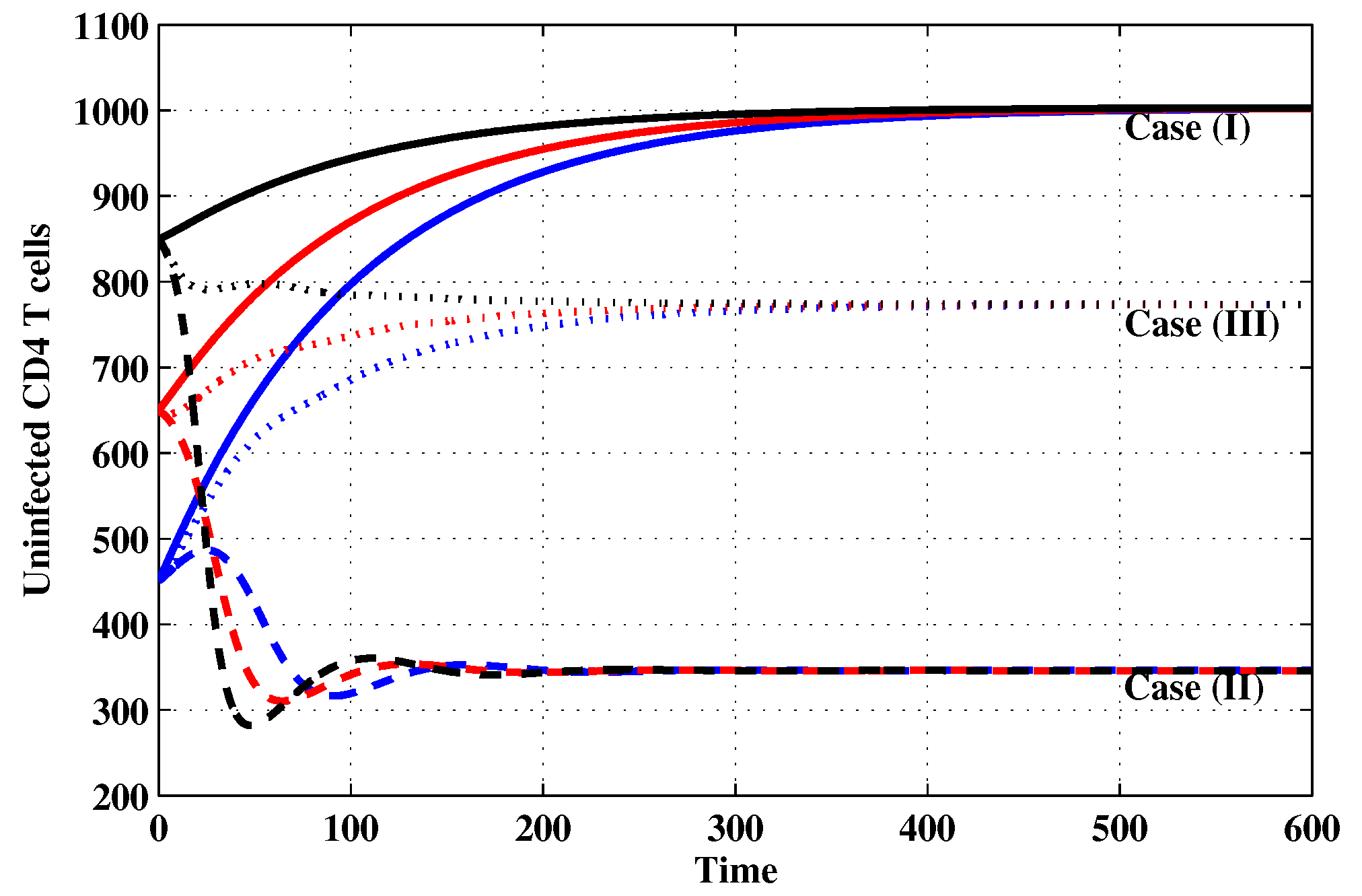
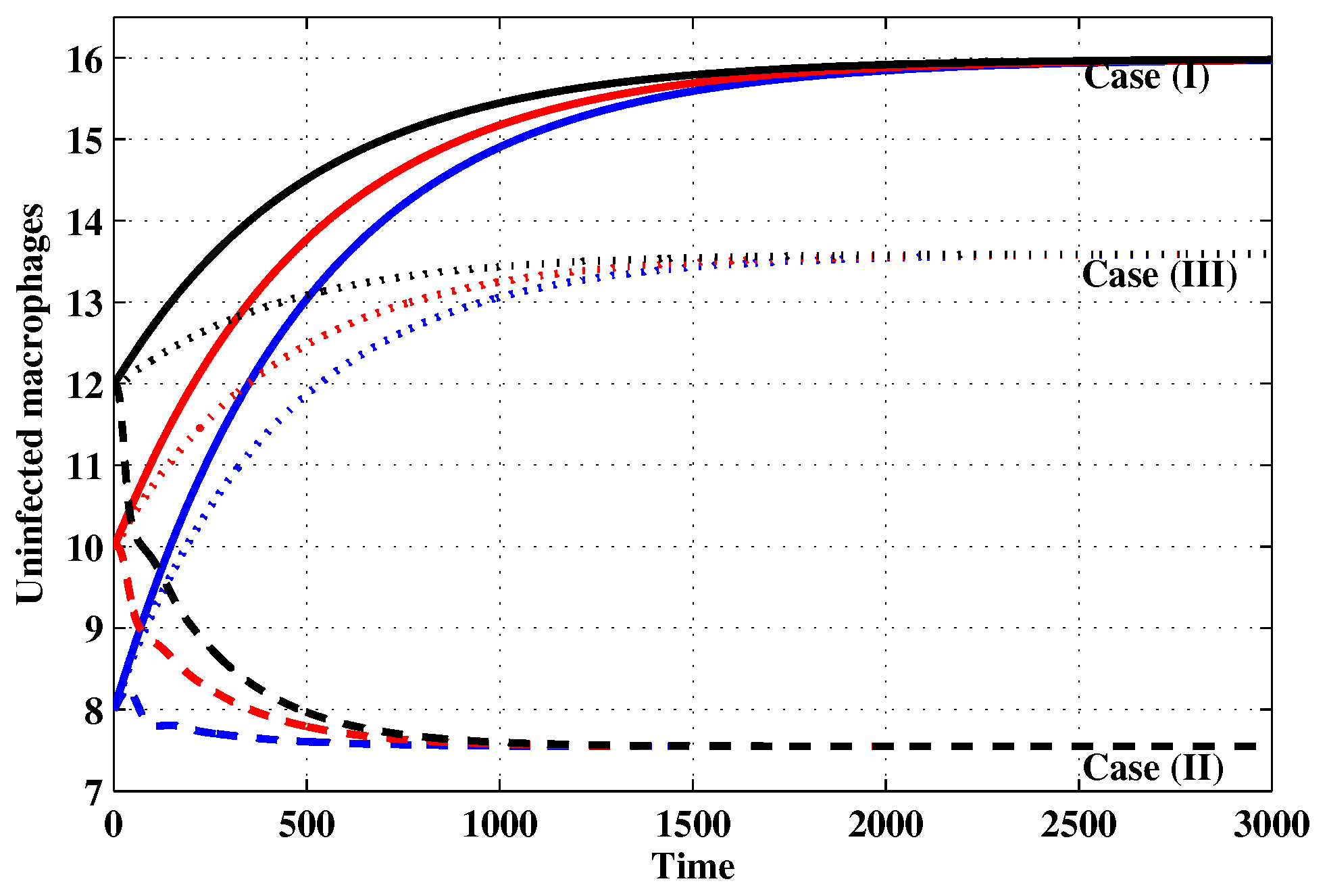
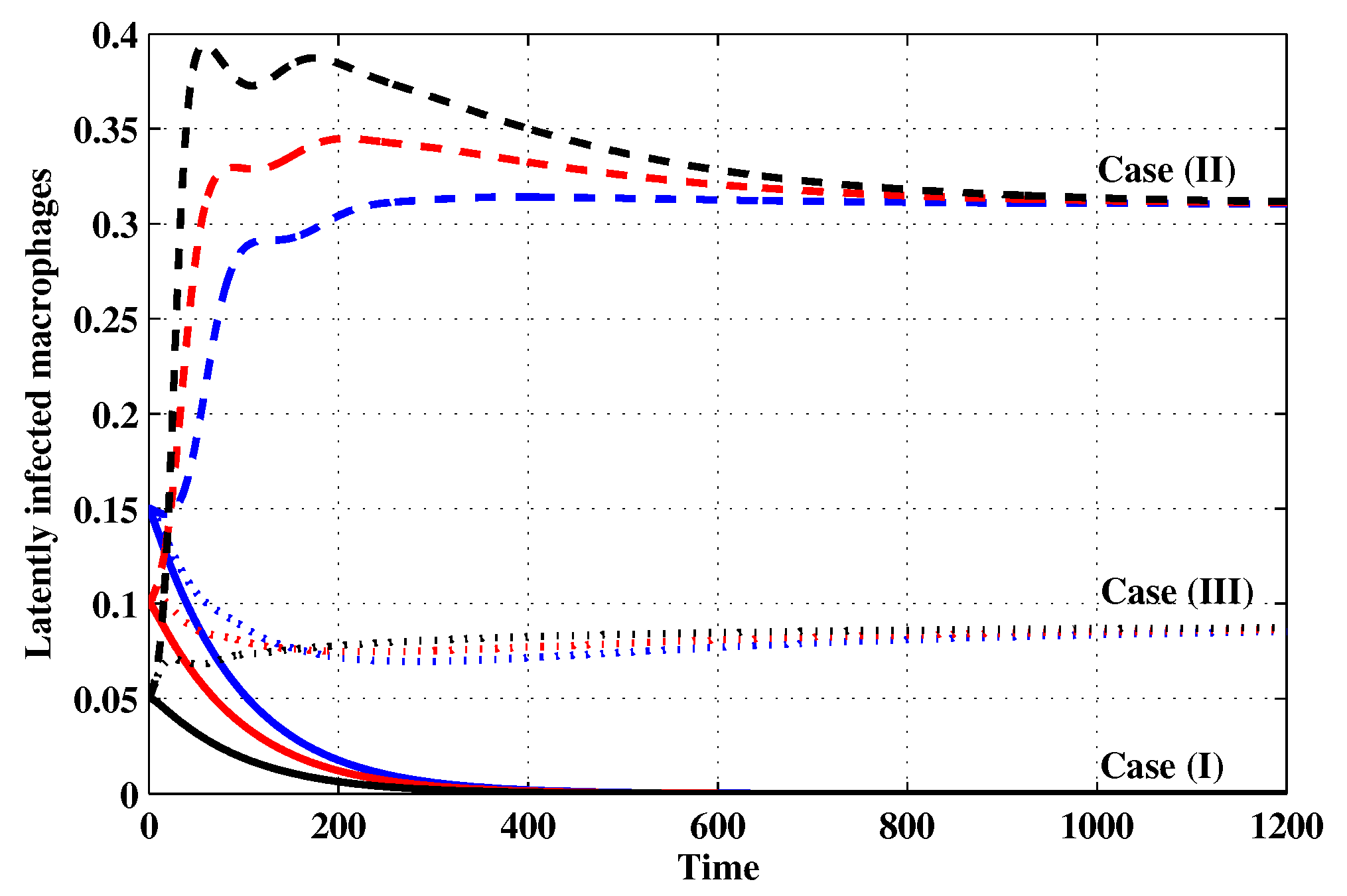
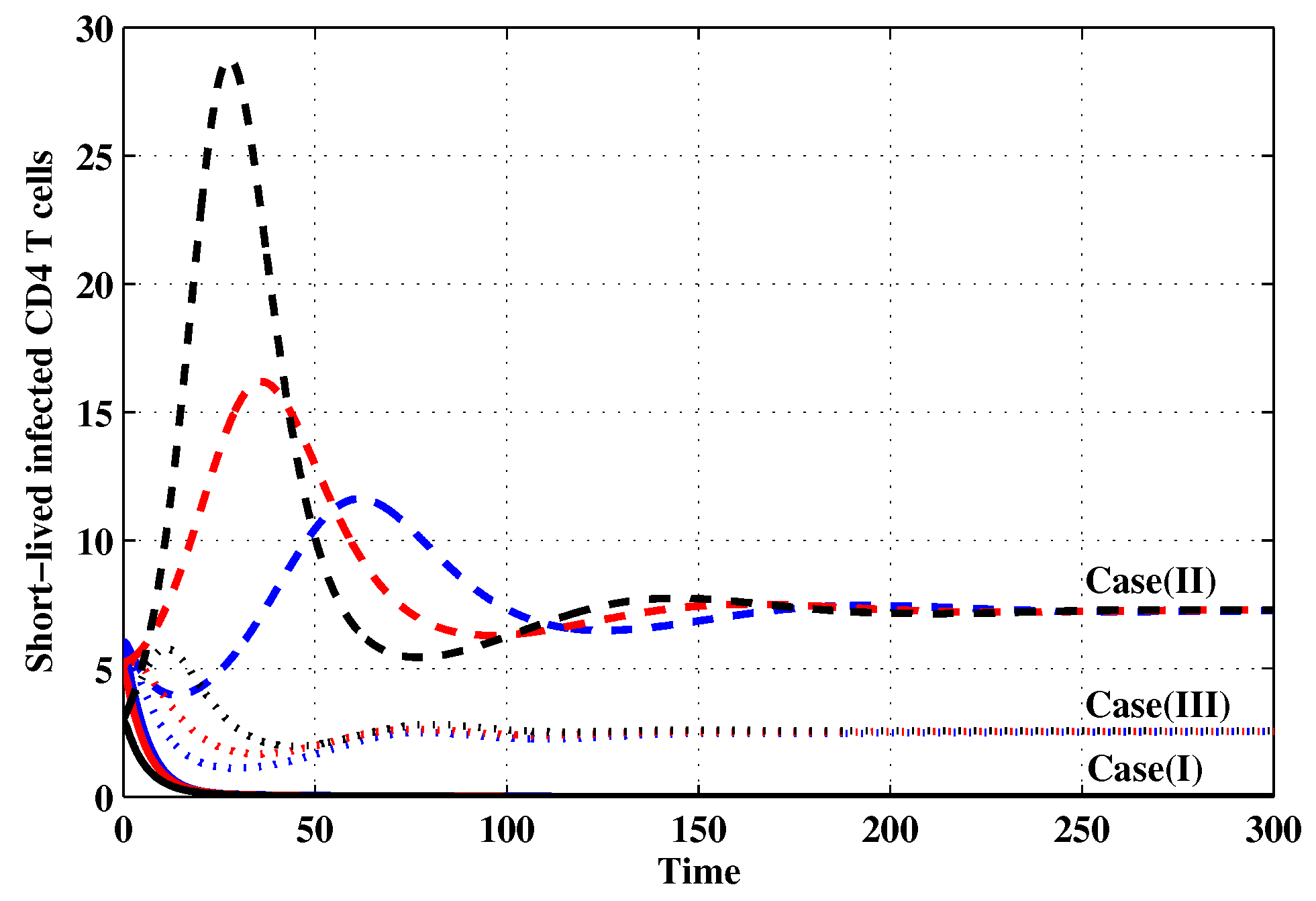
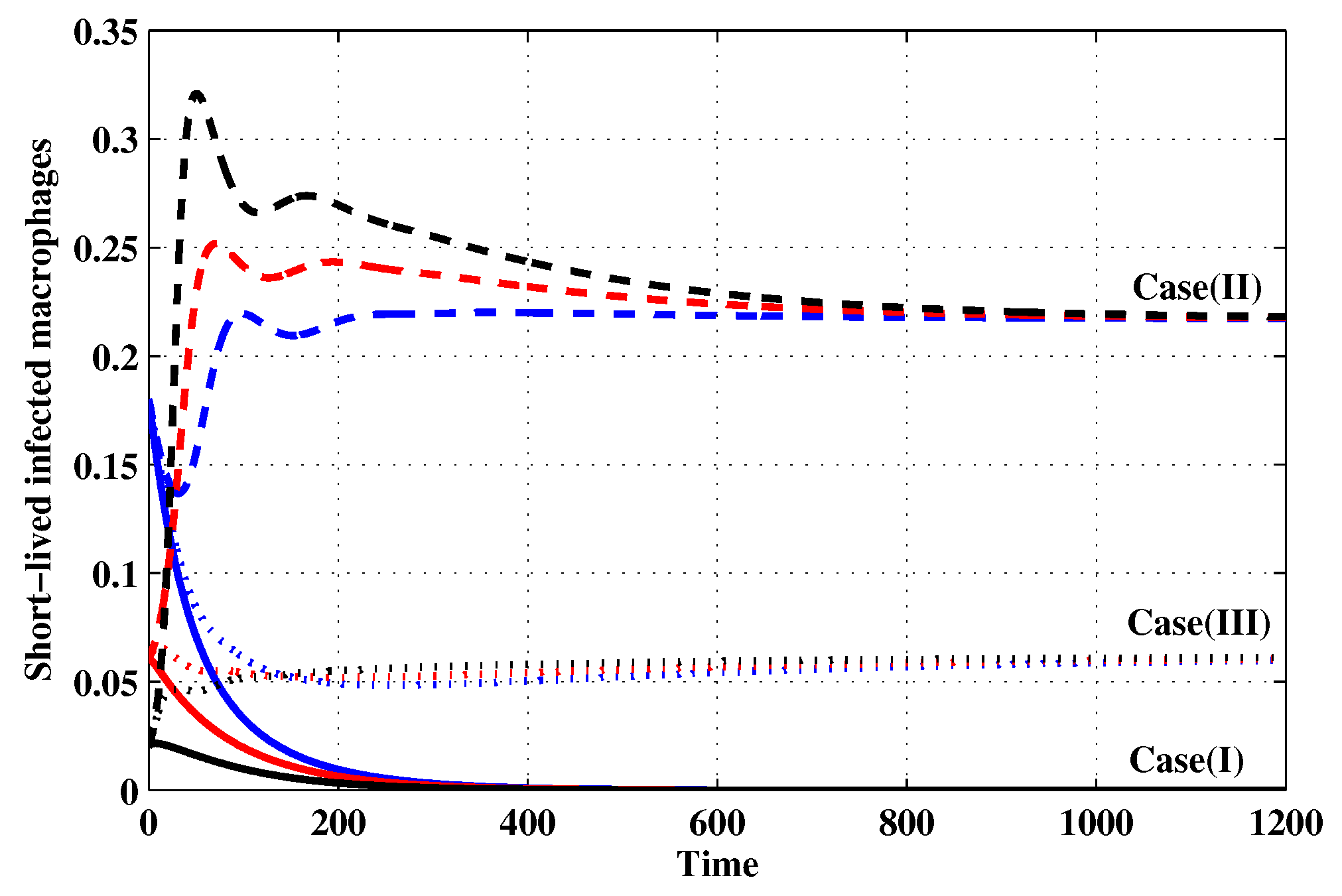
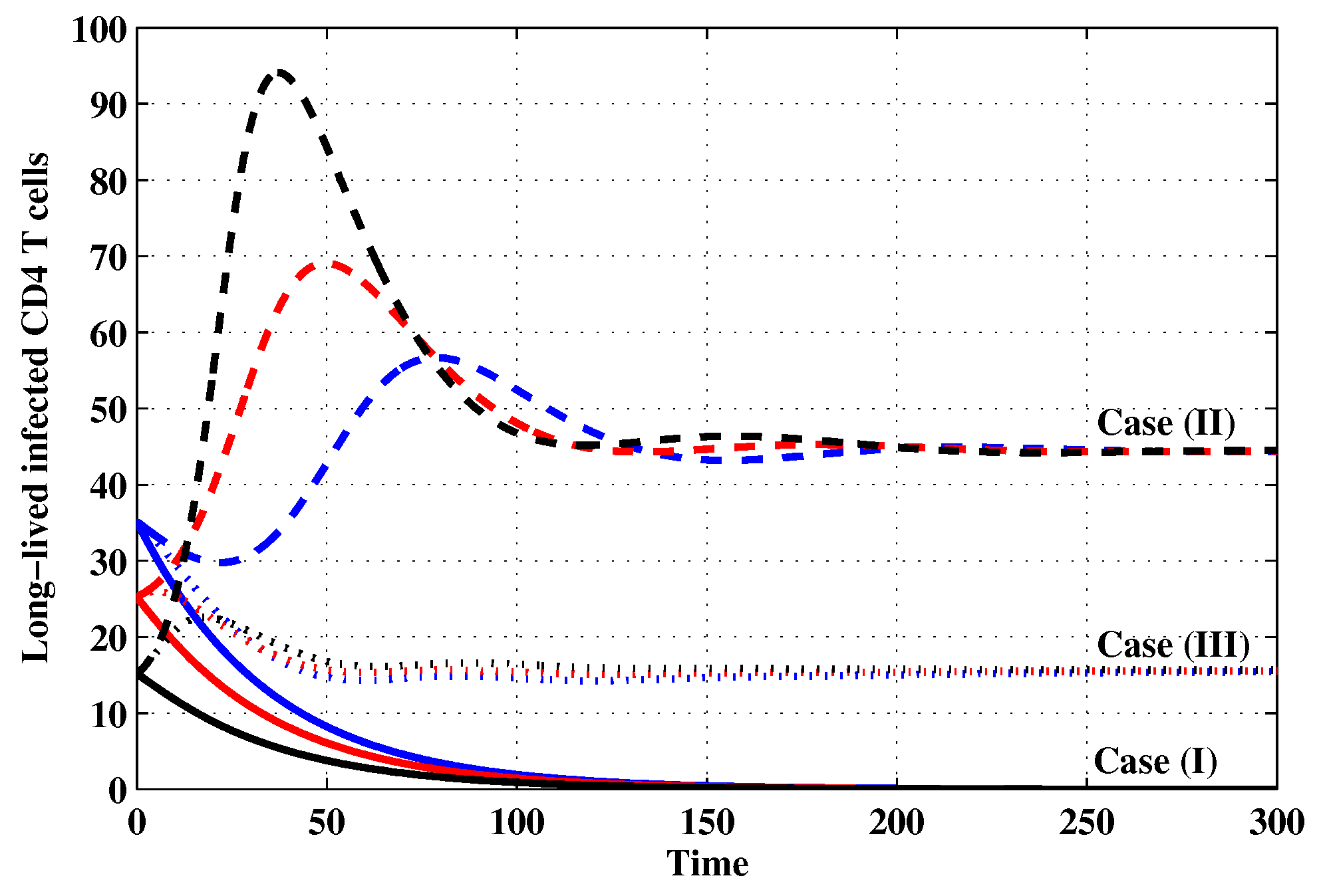
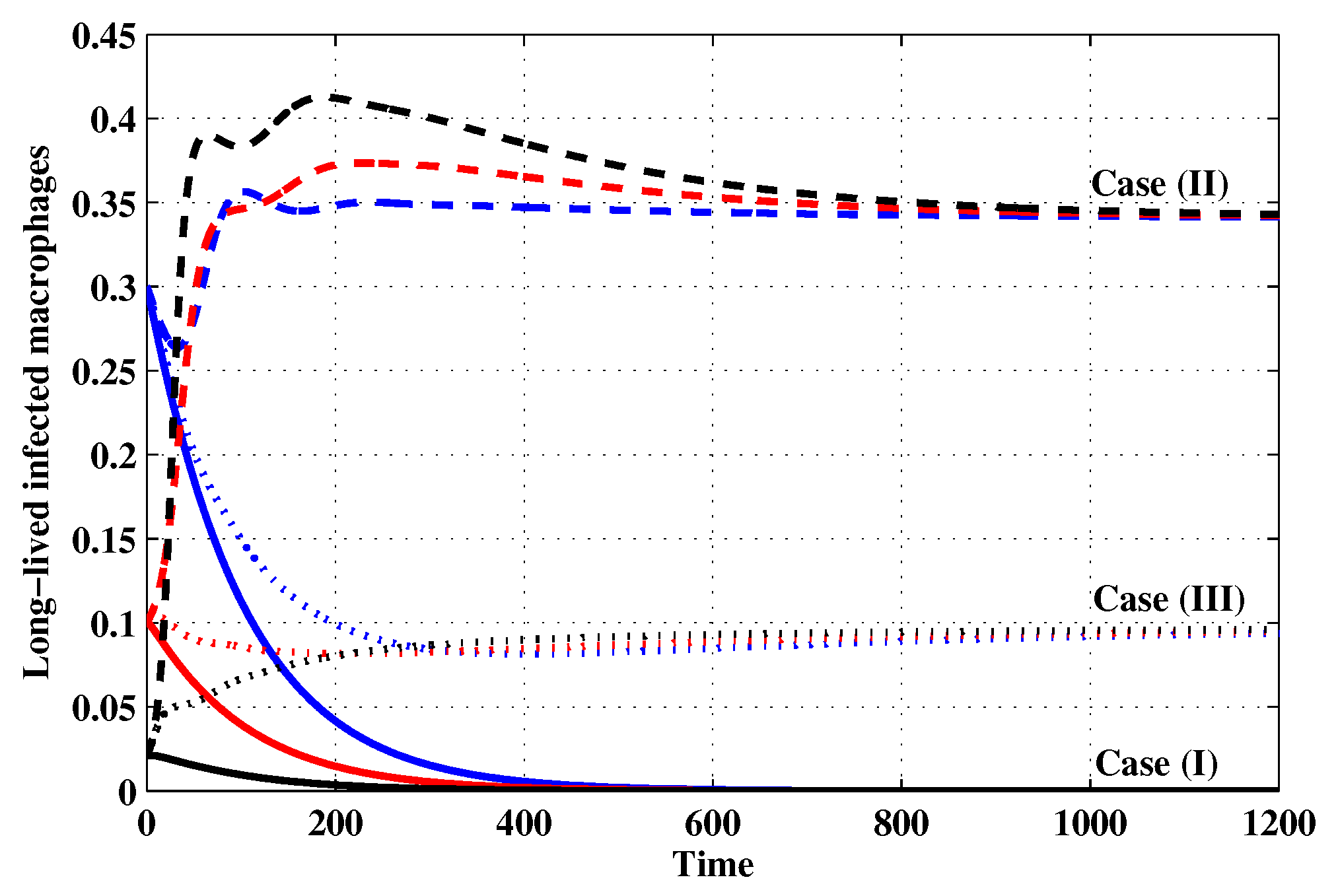
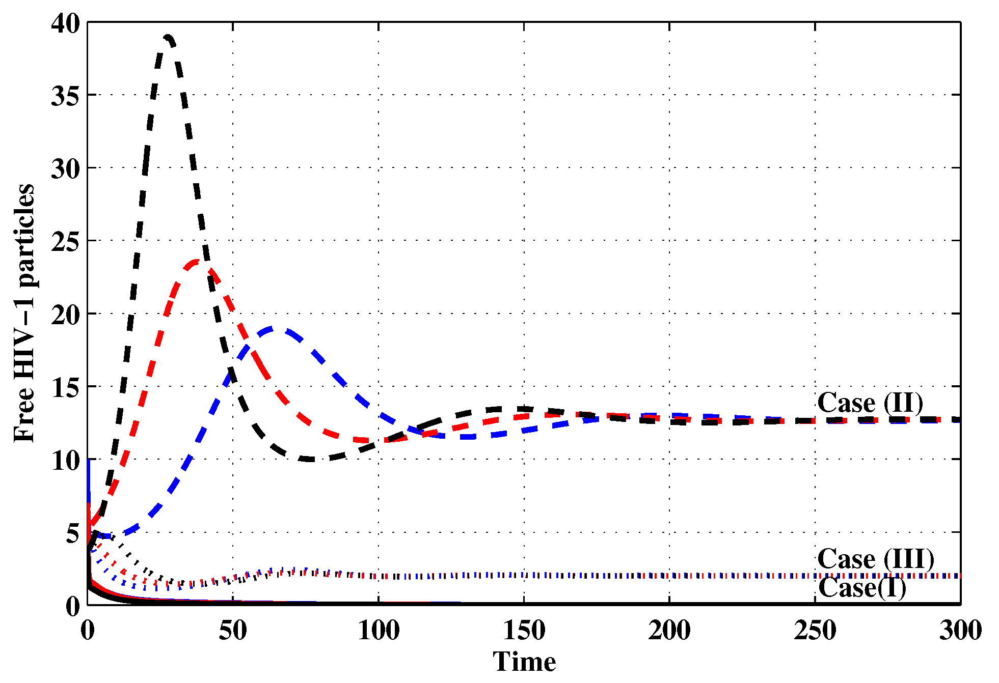
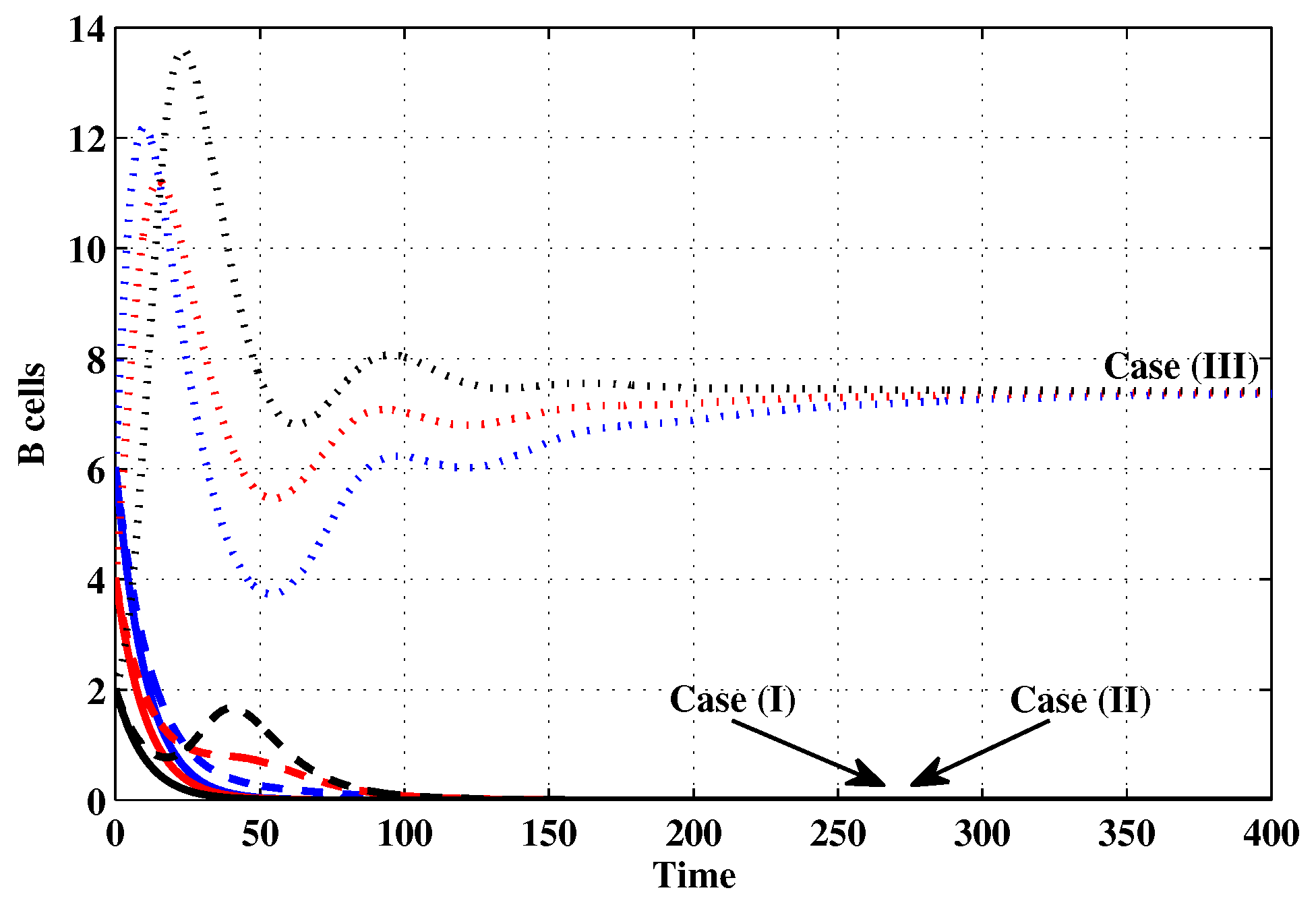
4.1. Stability of the Equilibria of the System

In this part of simulation, we choose three different initial conditions:
IC1: 
( s 1 , s 2 , w 1 , w 2 , y 1 , y 2 , u 1 , u 2 , p , x ) ( θ ) = ( 450 , 8 , 6 , 0.15 , 6 , 0.18 , 35 , 0.3 , 10 , 6 ) ,
IC2: 
( s 1 , s 2 , w 1 , w 2 , y 1 , y 2 , u 1 , u 2 , p , x ) ( θ ) = ( 650 , 10 , 4 , 0.1 , 5 , 0.06 , 25 , 0.1 , 7 , 4 ) ,
IC3: 
( s 1 , s 2 , w 1 , w 2 , y 1 , y 2 , u 1 , u 2 , p , x ) ( θ ) = ( 850 , 12 , 2 , 0.05 , 3 , 0.02 , 15 , 0.02 , 4 , 2 ) , θ τ , 0 .
We study three cases by choosing ε 1 , ε 2 , τ and r. In Figure 1, Figure 2, Figure 3, Figure 4, Figure 5, Figure 6, Figure 7, Figure 8, Figure 9 and Figure 10, we want to confirm our global stability results given in Theorems 1–3, by showing that any initial points taken from a feasible set the trajectory of the system will tend to one of the three equilibria of the system.
Case (I): Choose ε 1 = 0.7 , ε 2 = 0.7 , τ = 0.85 and r = 0.009 , which gives R 0 = 0.2778 < 1 and R 1 = 0.1156 < 1 . Figure 1, Figure 2, Figure 3, Figure 4, Figure 5, Figure 6, Figure 7, Figure 8, Figure 9 and Figure 10 show that the concentrations of the uninfected CD4 + T cells and macrophages are increasing and reach the values s 1 0 = 1003.3 and s 2 0 = 16 , respectively. In other words, concentrations of short-lived, long-lived and latently infected cells as well as HIV particles and B cells converge to zero. This confirms the result of Theorem 1, which is Π 0 is globally asymptotically stable. As a result, the HIV is removed from the plasma.
Case (II): We take ε 1 = 0.2 , ε 2 = 0.3 , τ = 0.5 and r = 0.004 . For these values, R 1 = 0.6692 < 1 < R 0 = 3.1775 . From Figure 1, Figure 2, Figure 3, Figure 4, Figure 5, Figure 6, Figure 7, Figure 8, Figure 9 and Figure 10, we can see that for IC1–IC3 the state Π 1 = ( 346.147 , 7.549 , 6.054 , 0.31 , 7.265 , 0.217 , 44.397 , 0.341 , 12.688 , 0.0 ) is reached, where the HIV infection is chronic and the antibody immune system is inactive. Hence, Theorem 2 is confirmed.
Case (III): ε 1 = 0.2 , ε 2 = 0.3 , τ = 0.5 and r = 0.05 . Then, we calculate R 0 = 3.1775 > 1 and R 1 = 2.4497 > 1 . From Figure 1, Figure 2, Figure 3, Figure 4, Figure 5, Figure 6, Figure 7, Figure 8, Figure 9 and Figure 10, we see that for IC1–IC3, the state Π 2 = ( 773.46 , 13.594 , 2.132 , 0.088 , 2.559 , 0.062 , 15.638 , 0.097 , 2 , 7.405 ) is reached, where the HIV infection is chronic and the antibody immune system is active. Thus, Theorem 3 is confirmed.
We mention that, R 0 does not depends on the parameters ω , r and μ . This fact seems to suggest that antibody immune response does not play a role in clearing the HIV particles. From above, we can see that R 1 can be increased by increasing the value of r. When we compare the Cases (II) and (III), we can see from the figures that, when the antibody immune response is activated (i.e., R 1 > 1 ), it reduces the concentrations of HIV free particles and infected (short-lived, long-lived and latent) cells and increases the concentration of uninfected target cells. It means that the antibody immune response can play a significant role in controlling the infection.

Effect of the Drug Efficacy on the Stability of the System

We take ε 1 = ε 2 = ε , τ = 0.5 , and r = 0.05 . In Table 2, we present the values of R 0 and R 1 for selected values of ε . It is seen that the values of R 0 and R 1 are decreased as ε is increased. Using the values of the parameters given in Table 1, we obtain the following cases:
(i)
if 0 ε < 0.54636 , then R 1 > 1 , Π 2 exists and it is globally asymptotically stable,
(ii)
if 0.54636 ε < 0.58032 , then R 1 1 , Π 1 exists and it is globally asymptotically stable and
(iii)
if 0.58032 ε 1 , then R 0 1 and Π 0 is globally asymptotically stable.
Thus, the results of Theorems 1–3 and the numerical results are compatible. Therefore, we can say that treatment with sufficient drug efficacy can successfully clear the virus from the plasma.

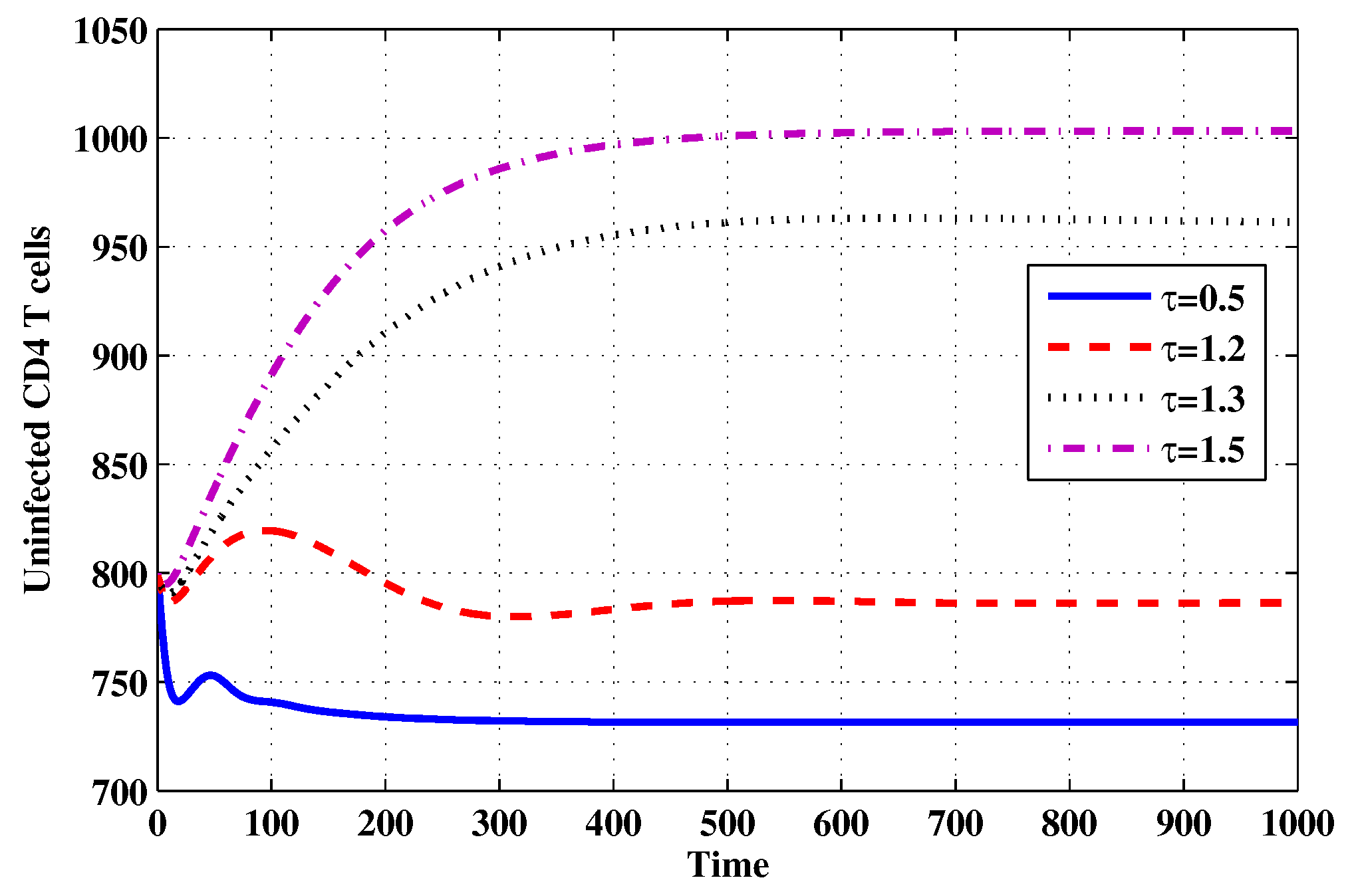
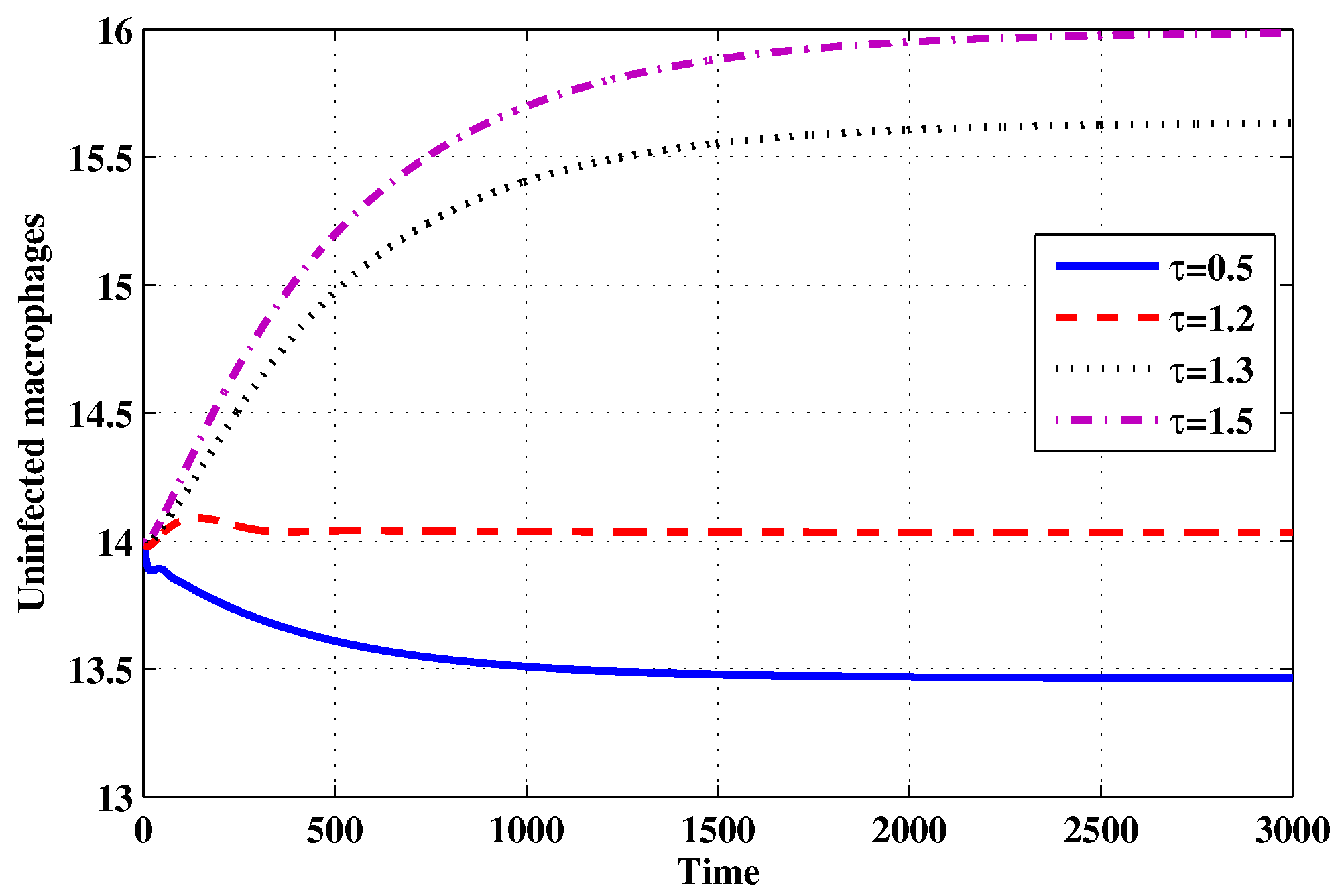
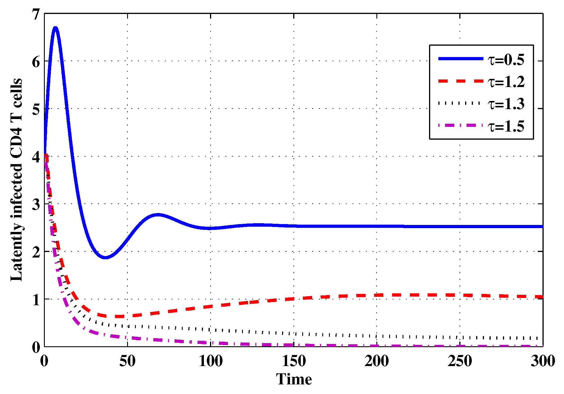
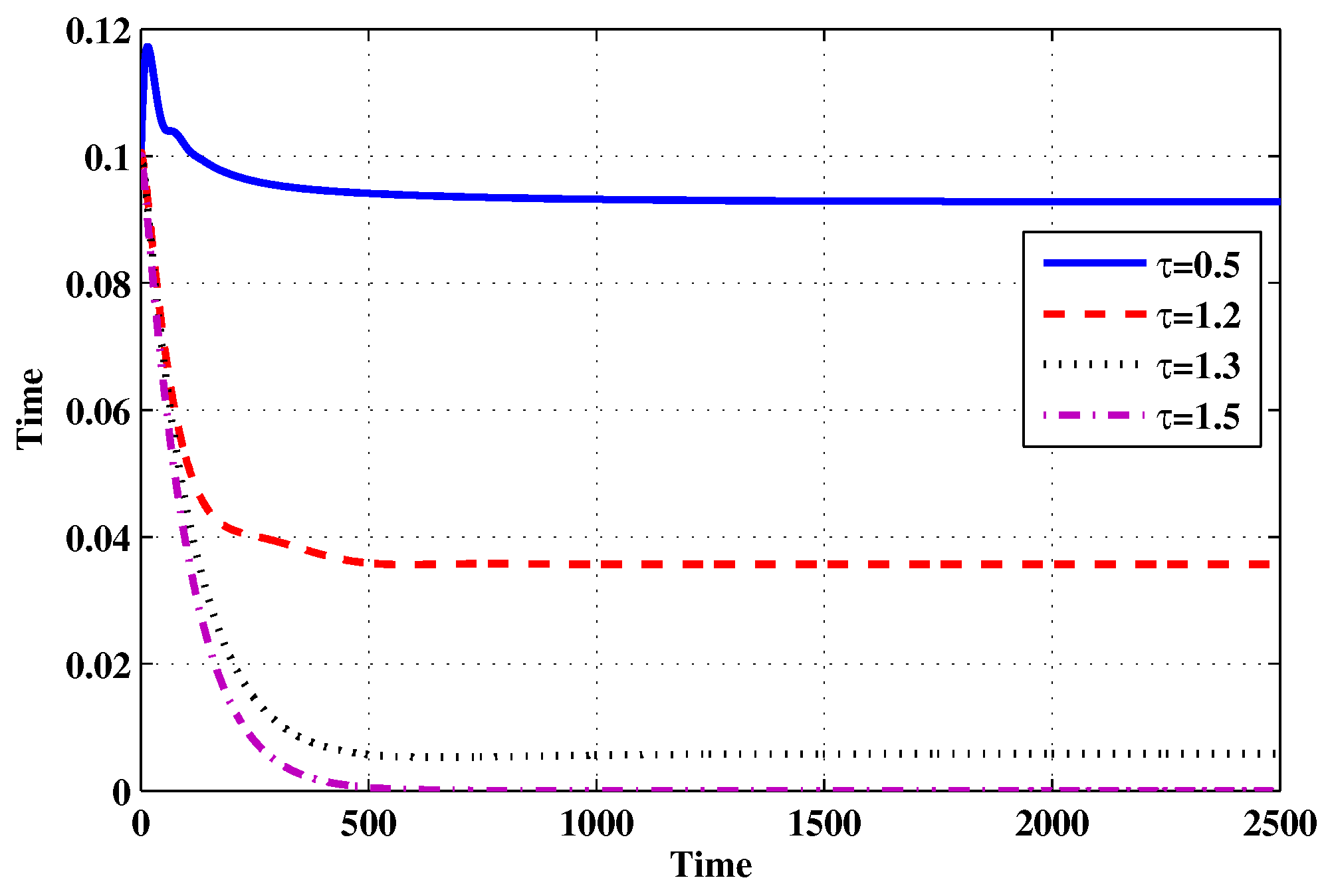
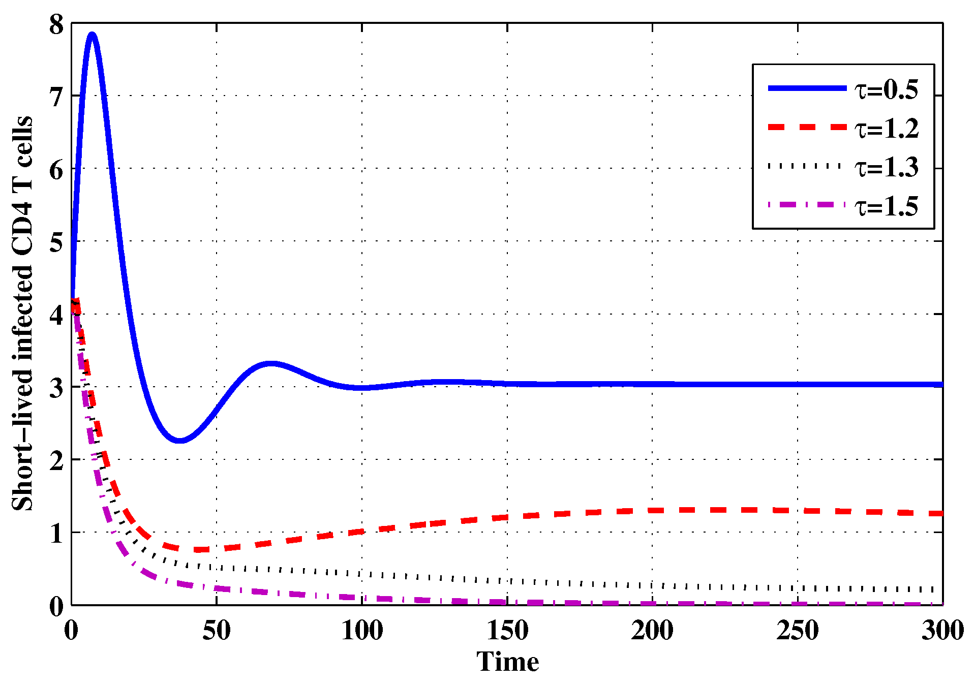
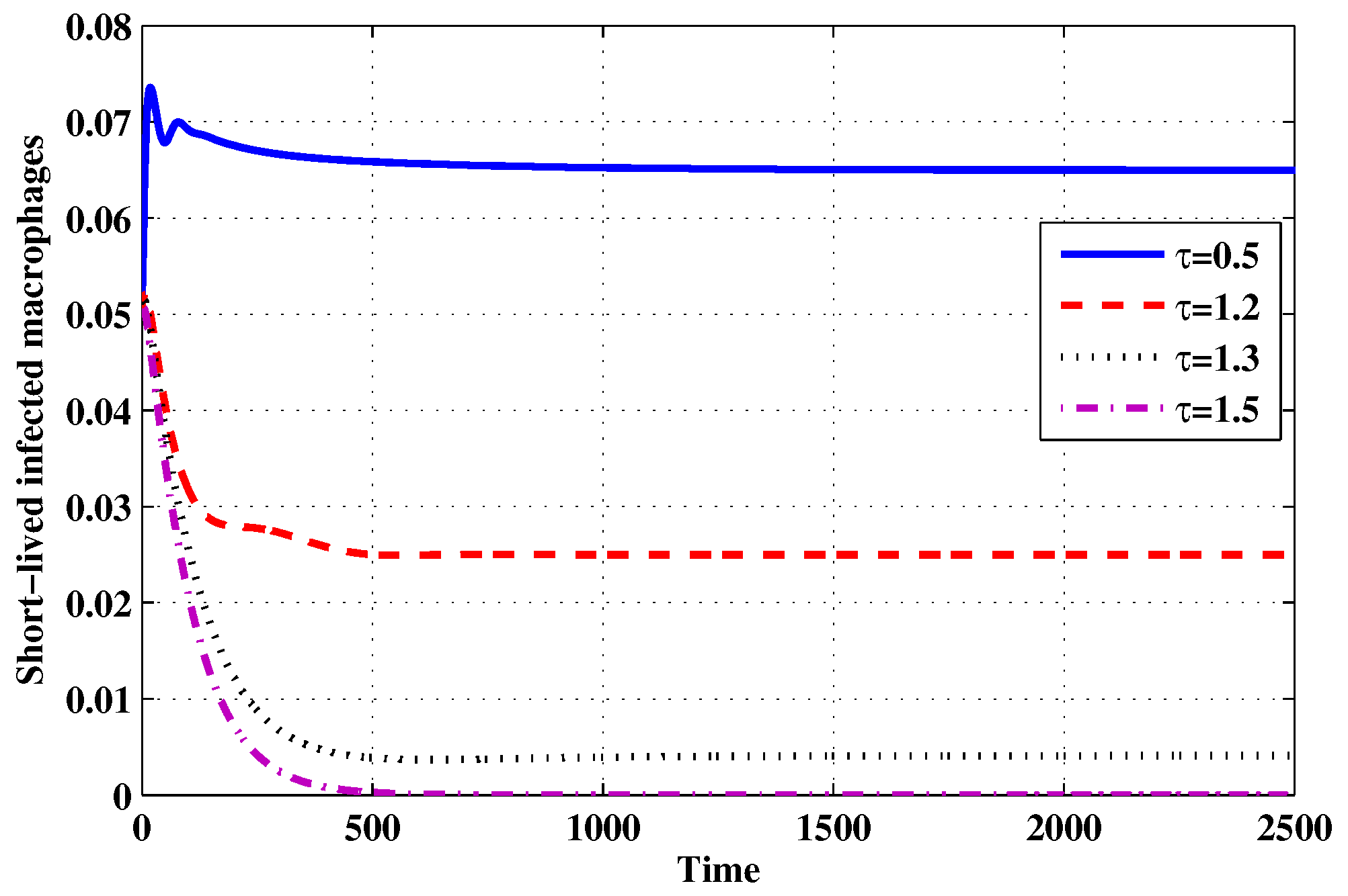
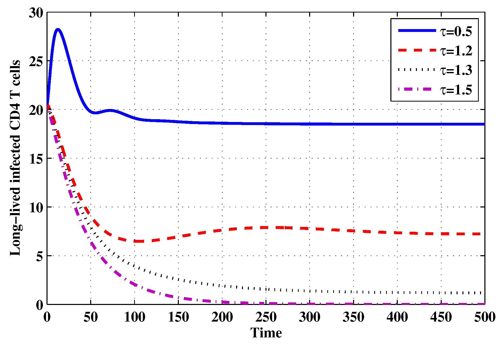
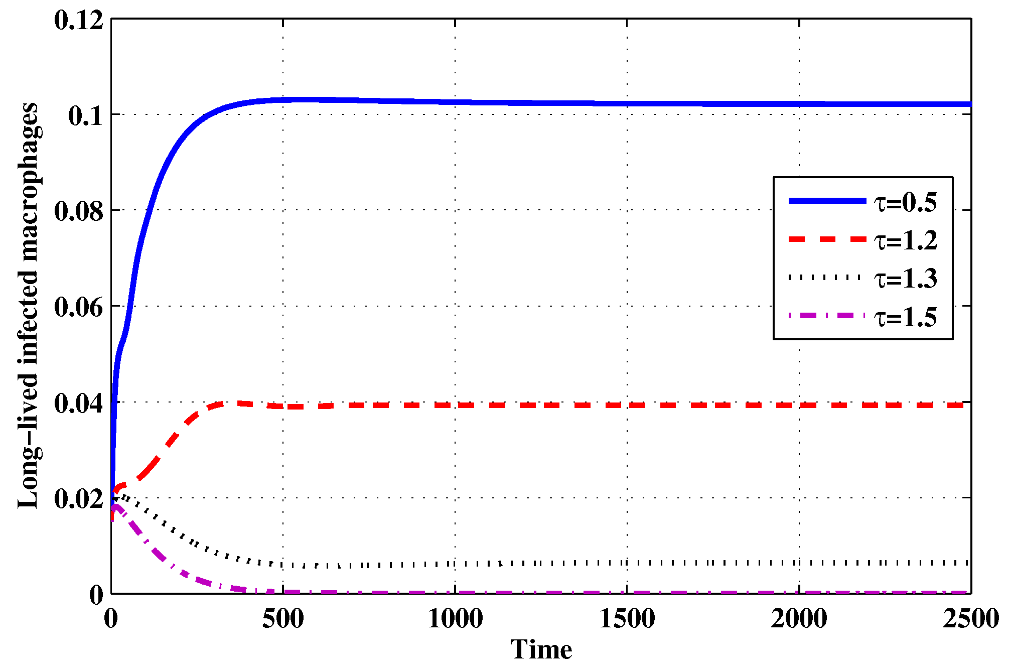
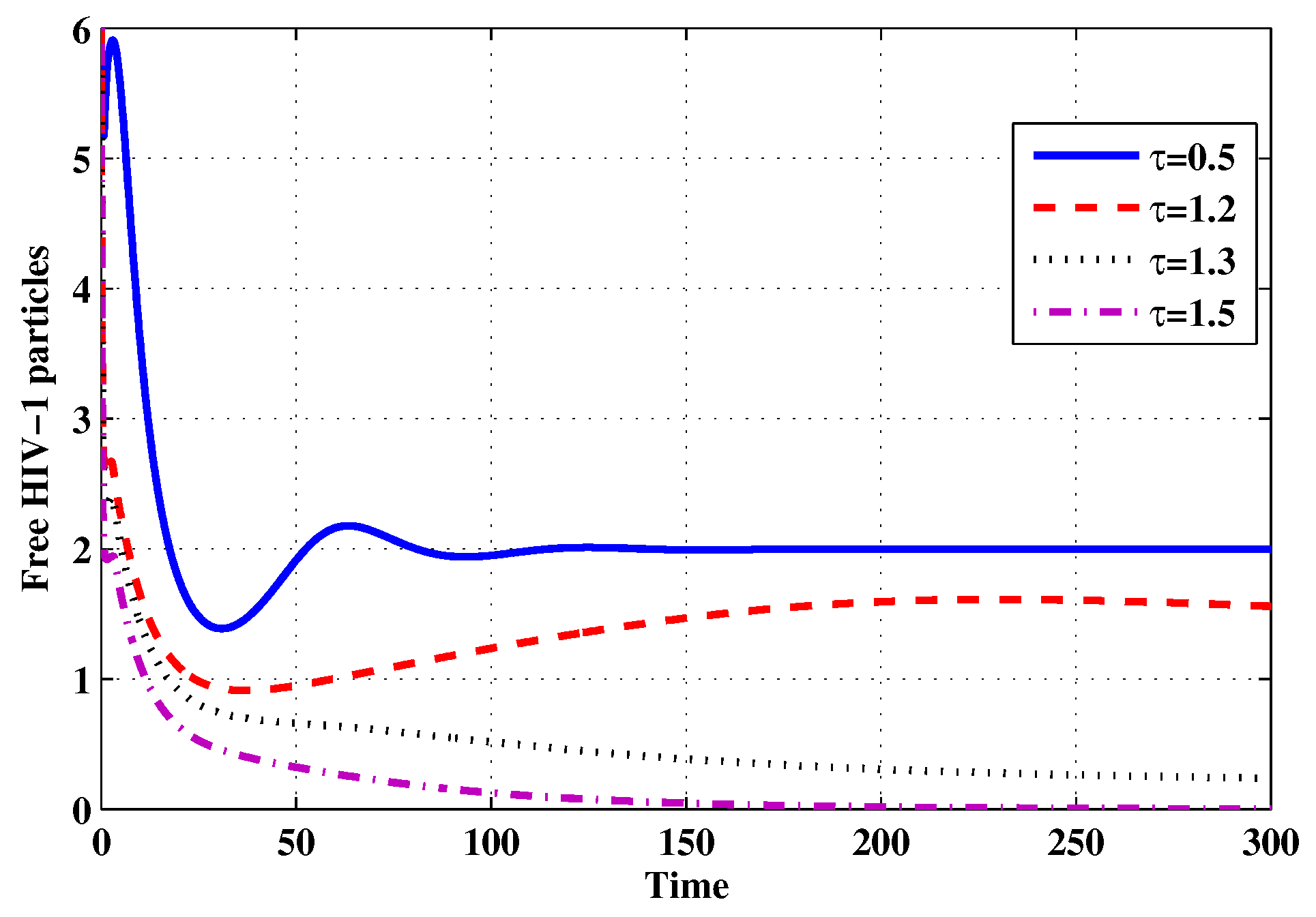
4.2. Effect of the Time Delay on the Stability of the System

Choose ε 1 = ε 2 = 0 , and r = 0.05 . The initial conditions are considered to be ( s 1 , s 2 , w 1 , w 2 , y 1 , y 2 , u 1 , u 2 , p , x ) ( θ ) = ( 800 , 14 , 4 , 0.1 , 4 , 0.05 , 20 , 0.015 , 6 , 5 ) , θ τ , 0 . Figure 11, Figure 12, Figure 13, Figure 14, Figure 15, Figure 16, Figure 17, Figure 18, Figure 19 and Figure 20 and Table 3 show the effect of the time delay parameter τ on the stability of Π 0 , Π 1 and Π 2 . It can be seen that, as τ is increased, the concentration of the uninfected target cells is increased, while the concentrations of short-lived, long-lived and latently infected cells, free HIV particles and B cells are decreased. From Figure 11, Figure 12, Figure 13, Figure 14, Figure 15, Figure 16, Figure 17, Figure 18, Figure 19 and Figure 20, we can see that, in the case of smaller values of τ , the trajectory of system will converge to Π 2 . When the value of τ is increased, the trajectory will converge to Π 1 and finally approach Π 0 . From a biological point of view, the intracellular time delay plays a similar role as the anti-HIV drugs in eliminating the virus. We observe that sufficiently large delay suppresses viral replication and clears the virus from the body. This gives us some suggestions on new drugs to prolong the increase in the intracellular delay period.

5. Discussion

All of the HIV infection mathematical models with three categories of infected cells, short-lived, long-lived and latent presented in the literature have studied the HIV infection and production in one class of target cells, CD4 + T cells. However, it has been reported in several papers that HIV can infect both CD4 + T cells and macrophages. In this paper, we have proposed an HIV infection model with three categories of infected cells and two classes of target cells, CD4 + T cells and macrophages. We have incorporated multiple distributed time delays to characterize the time between an HIV contacts an uninfected target cell and the creation of mature HIV particles. The effect of antibody immune response has been modeled. The production and removal rates of all compartments are represented by general nonlinear functions. The incidence rate of infection is also given by a general nonlinear function. The model can be seen as a generalization of several HIV dynamics models presented in the literature. We have shown that the solutions of the model are nonnegative and ultimately bounded, which ensures the well-posedness of the model. We have derived two threshold numbers R 0 (the basic reproduction number) and antibody immune response activation number R 1 , which determine the stability of the three equilibria of the model. We have investigated the global stability of the equilibria of the model by using Lyapunov method and LaSalle’s invariance principle. We have proven that (i) if R 0 1 , then the infection-free equilibrium Π 0 is globally asymptotically stable and the HIV is predicted to be completely cleared from the HIV infected patients, (ii) if the antibody-inactivated infection equilibrium Π 1 exists then it is globally asymptotically stable and a chronic HIV infection with inactive antibody immunity is attained, and (iii) if R 1 > 1 , then the antibody-activated infection equilibrium Π 2 is globally asymptotically stable and a chronic HIV infection with active antibody immunity is attained. We have conducted numerical simulations and have shown that both the theoretical and numerical results are consistent.
Our analysis extends the results presented in [27], where the global stability was analyzed for a model with one target cell population. When we consider the HIV dynamics with only one class of target cells, CD4 + T cells, then model (10)–(15) leads to the following model:
s ˙ 1 t = ρ 1 δ 1 s 1 t + B s 1 t 1 s 1 t s max ( 1 ε 1 ) λ ¯ 1 s 1 t p t ,
w ˙ 1 t = ( 1 ε 1 ) λ ¯ 11 e μ 11 τ 11 s 1 t τ 11 p t τ 11 ( α 1 + β 1 ) w 1 t ,
y ˙ 1 t = ( 1 ε 1 ) λ ¯ 21 e μ 21 τ 21 s 1 t τ 21 p t τ 21 + α 1 w 1 t η 1 y 1 t ,
u ˙ 1 t = ( 1 ε 1 ) λ ¯ 31 e μ 31 τ 31 s 1 t τ 31 p t τ 31 ν 1 u 1 t ,
p ˙ t = ( 1 ε 2 ) N 1 ¯ η 1 e μ 41 τ 41 y 1 t τ 41 + ( 1 ε 2 ) M 1 ¯ ν 1 e μ 51 τ 51 u 1 t τ 51 g p t μ p t x t ,
x ˙ t = r p t x t ω x t .
Let us define the overall HAART effect as ε e = ε 1 + ε 2 ε 1 ε 2 [39]. If ε e = 0 ,then the HAART has no effect, if ε e = 1 , the HIV-1 growth is completely halted. Consequently, the basic reproduction number for system (37)–(42) is given by
R 0 C ( ε e ) = ( 1 ε e ) N ¯ 1 A ¯ 1 e μ 41 τ 41 + M ¯ 1 λ ¯ 31 ( α 1 + β 1 ) e μ 31 τ 31 μ 51 τ 51 g ( α 1 + β 1 ) s 1 0 , A ¯ 1 = α 1 λ ¯ 11 e μ 11 τ 11 + ( α 1 + β 1 ) λ ¯ 21 e μ 21 τ 21 .
For comparison purposes, we assume that h = f = 1 ; then, the basic reproduction number for system (27)–(36) can be written as: R 0 = R 0 C M ( ε e ) = R 0 C ( ε e ) + R 0 M ( ε e ) where:
R 0 M ( ε e ) = ( 1 ε e ) N ¯ 2 A ¯ 2 e μ 42 τ 42 + M ¯ 2 λ ¯ 32 ( α 2 + β 2 ) e μ 32 τ 32 μ 52 τ 52 g ( α 2 + β 2 ) s 2 0 , A ¯ 2 = α 2 λ ¯ 12 e μ 12 τ 12 + ( α 2 + β 2 ) λ ¯ 22 e μ 22 τ 22 ,
where R 0 M ( ε e ) is the basic reproduction number of a model that describes the HIV dynamics with only macrophages and neglecting the CD4 + T cells. For system (37)–(42), one can determine drug efficacy ε e C such that R 0 C ( ε e C ) = 1 as:
ε e C = max R 0 C ( 0 ) 1 R 0 C ( 0 ) , 0 .
Therefore, if ε e C ε e 1 , then R 0 C ( ε e C ) 1 . For system (27)–(36), one can also determine the drug efficacy ε e C M such that R 0 C M ( ε e C M ) = 1 as:
ε e C M = max R 0 C M ( 0 ) 1 R 0 C M ( 0 ) , 0 .
Therefore, if ε e C M ε e 1 , then R 0 C M ( ε e C M ) 1 .
Assume that R 0 C ( 0 ) > 1 , then Π 0 of system (37)–(42) is unstable in the absence of treatment. Since R 0 C ( 0 ) < R 0 C M ( 0 ) , then ε e C < ε e C M . Therefore, if we apply drugs with ε e such that ε e C ε e < ε e C M , this guarantees that R 0 C ( ε e ) 1 and the system (37)–(42) can be stabilized around Π 0 ; however, R 0 C M ( ε e ) > 1 and then Π 0 of (27)–(36) is unstable. Therefore, more accurate drug efficacy ε e is determined when using the model with two classes of target cells. This shows the importance of considering the effect of the macrophages in the HIV dynamics.

Author Contributions

Conceptualization, A.M.E. and E.K.E.; methodology, A.M.E.; analysis, E.K.E.; writing-original draft preparation, E.K.E.; writing-review and editing, E.K.E.; simulation, E.K.E.; supervision, A.M.E.

Funding

This research received no external funding.

Conflicts of Interest

The authors declare no conflict of interest.

Appendix A

The following equalities will be used in the proofs of the Theorems 2 and 3:
ln Υ i ( s i t τ , p t τ ) Υ i ( s i , p ) = ln ψ 1 i ( w ^ i ) Υ i ( s i t τ , p t τ ) ψ 1 i ( w i ) Υ i ( s ^ i , p ^ ) + ln Υ i ( s ^ i , p ^ ) Υ i ( s i , p ^ ) + ln ψ 41 ( p ) Υ i ( s i , p ^ ) ψ 41 ( p ^ ) Υ i ( s i , p ) + ln ψ 41 ( p ^ ) ψ 2 i ( y i ) ψ 41 ( p ) ψ 2 i ( y ^ i ) + ln ψ 2 i ( y ^ ) ψ 1 i ( w i ) ψ 2 i ( y i ) ψ 1 i ( w ^ i ) , ln Υ i ( s i t τ , p t τ ) Υ i ( s i , p ) = ln ψ 2 i ( y ^ i ) Υ i ( s i t τ , p t τ ) ψ 2 i ( y i ) Υ i ( s ^ i , p ^ ) + ln Υ i ( s ^ i , p ^ ) Υ i ( s i , p ^ ) + ln ψ 41 ( p ^ ) ψ 2 i ( y i ) ψ 41 ( p ) ψ 2 i ( y ^ i ) + ln ψ 41 ( p ) Υ i ( s i , p ^ ) ψ 41 ( p ^ ) Υ i ( s i , p ) , ln Υ i ( s i t τ , p t τ ) Υ i ( s i , p ) = ln ψ 3 i ( u ^ i ) Υ i ( s i t τ , p t τ ) ψ 3 i ( u i ) Υ i ( s ^ i , p ^ ) + ln Υ i ( s ^ i , p ^ ) Υ i ( s i , p ^ ) + ln ψ 3 i ( u i ) ψ 41 ( p ^ ) ψ 3 i ( u ^ i ) ψ 41 ( p ) + ln ψ 41 ( p ) Υ i ( s i , p ^ ) ψ 41 ( p ^ ) Υ i ( s i , p ) , ln ψ 2 i ( y i t τ ) ψ 2 i ( y i ) = ln ψ 2 i ( y i t τ ) ψ 41 ( p ^ ) ψ 2 i ( y ^ i ) ψ 41 ( p ) + ln ψ 2 i ( y ^ i ) ψ 41 ( p ) ψ 2 i ( y i ) ψ 41 ( p ^ ) , ln ψ 3 i ( u i t τ ) ψ 3 i ( u i ) = ln ψ 3 i ( u i t τ ) ψ 41 ( p ^ ) ψ 3 i ( u ^ i ) ψ 41 ( p ) + ln ψ 3 i ( u ^ i ) ψ 41 ( p ) ψ 3 i ( u i ) ψ 41 ( p ^ ) .
Proof of Lemma 1.
Denote k = ( s 1 , s 2 , w 1 , w 2 , y 1 , y 2 , u 1 , u 2 , p , x ) T , L = ( L 1 , L 2 , , L 10 ) T . Then, systems (10)–(15) can be written as k ˙ t = L k t , where
L k t = L 1 k t L 2 k t . . . L 10 k t ,
L = π 1 ( s 1 t ) λ 1 Υ 1 ( s 1 t , p t ) π 2 ( s 2 t ) λ 2 Υ 2 ( s 2 t , p t ) λ 11 0 h 11 Θ 11 Υ 1 ( s 1 t τ , p t τ ) d τ ( α 1 + β 1 ) ψ 11 ( w 1 t ) λ 12 0 h 12 Θ 12 Υ 2 ( s 2 t τ , p t τ ) d τ ( α 2 + β 2 ) ψ 12 ( w 2 t ) λ 21 0 h 21 Θ 21 Υ 1 ( s 1 t τ , p t τ ) d τ + α 1 ψ 11 ( w 1 t ) η 1 ψ 21 ( y 1 t ) , λ 22 0 h 22 Θ 22 Υ 2 ( s 2 t τ , p t τ ) d τ + α 2 ψ 12 ( w 2 t ) η 2 ψ 22 ( y 2 t ) , λ 31 0 h 31 Θ 31 Υ 1 ( s 1 t τ , p t τ ) d τ ν 1 ψ 31 ( u 1 t ) λ 32 0 h 32 Θ 32 Υ 2 ( s 2 t τ , p t τ ) d τ ν 2 ψ 32 ( u 2 t ) i = 1 2 N i η i 0 h 4 i Θ 4 i ψ 2 i ( y i t τ ) d τ + M i ν i 0 h 5 i Θ 5 i ψ 3 i ( u i t τ ) d τ g ψ 41 ( p t ) μ ψ 41 ( p t ) ψ 42 ( x t ) , r ψ 41 ( p t ) ψ 42 ( x t ) ω ψ 42 ( x t ) .
We have
L j k t k t R > 0 10 0 , j = 1 , , 10 .
Applying Lemma 2 in [40], we get k ( t ) R 0 10 for all t 0 .
Equation (10) implies that lim t sup s i t M 1 i , where M 1 i = b i b ¯ i . Let
G i ( t ) = N i 0 h 1 i Θ 1 i ( τ ) s i ( t τ ) d τ + N i 0 h 2 i Θ 2 i ( τ ) s i ( t τ ) d τ + M i 0 h 3 i Θ 3 i ( τ ) s i ( t τ ) d τ + N i w i ( t ) + N i y i ( t ) + M i u i ( t ) ,
then
G ˙ i ( t ) = N i 0 h 1 i Θ 1 i ( τ ) π i ( s i t τ ) λ i Υ i ( s i t τ , p t τ ) d τ + N i 0 h 2 i Θ 2 i ( τ ) π i ( s i t τ ) λ i Υ i ( s i t τ , p t τ ) d τ + M i 0 h 3 i Θ 3 i ( τ ) π i ( s i t τ ) λ i Υ i ( s i t τ , p t τ ) d τ + N i λ 1 i 0 h 1 i Θ 1 i ( τ ) Υ i ( s i t τ , p t τ ) d τ α i + β i ψ 1 i ( w i ( t ) ) + N i λ 2 i 0 h 2 i Θ 2 i ( τ ) Υ i ( s i t τ , p t τ ) d τ + α i ψ 1 i ( w ( t ) ) η i ψ 2 i ( y i ( t ) ) + M i λ 3 i 0 h 3 i Θ 3 i ( τ ) Υ i ( s i t τ , p t τ ) d τ ν i ψ 3 i ( u i t ) N i 0 h 1 i Θ 1 i ( τ ) b i b i ¯ s i t τ d τ + N i 0 h 2 i Θ 2 i ( τ ) b i b i ¯ s i t τ d τ + M i 0 h 3 i Θ 3 i ( τ ) b i b i ¯ s i t τ d τ N i β i α 1 i w i ( t ) N i η i α 2 i y i ( t ) M i ν i α 3 i u i ( t ) b i N i F 1 i + N i F 2 i + M i F 3 i σ i N i 0 h 1 i Θ 1 i ( τ ) s i ( t τ ) d τ + N i 0 h 2 i Θ 2 i ( τ ) s i ( t τ ) d τ + M i 0 h 3 i Θ 3 i ( τ ) s i ( t τ ) d τ + N i w i ( t ) + N i y i ( t ) + M i u i ( t ) b i 2 N i + M i σ i G i ( t ) ,
where σ i = min { b i ¯ , β i α 1 i , η i α 2 i , ν i α 3 i } . Then, lim t sup G i ( t ) b i 2 N i + M i σ i and
lim t sup w i ( t ) b i 2 N i + M i N i σ i = M 2 i , lim t sup y i ( t ) b i 2 N i + M i N i σ i = M 2 i , lim t sup u i ( t ) b i 2 N i + M i M i σ i = M 3 i .
Moreover, we let G 3 ( t ) = p ( t ) + μ r x ( t ) . Then,
G ˙ 3 = i = 1 2 N i η i 0 h 4 i Θ 4 i ( τ ) ψ 2 i ( y i ( t τ ) ) d τ + M i ν i 0 h 5 i Θ 5 i ( τ ) ψ 3 i ( u i ( t τ ) ) d τ g ψ 41 ( p ) q ω r ψ 42 ( x ) i = 1 2 N i η i F 4 i ψ 2 i ( M 2 i ) + M i ν i F 5 i ψ 3 i ( M 3 i ) g α 41 p μ ω r α 42 x i = 1 2 N i η i F 4 i ψ 2 i ( M 2 i ) + M i ν i F 5 i ψ 3 i ( M 3 i ) σ 3 G 3 ( t ) ,
where σ 3 = min { g α 41 , ω α 42 } . Hence,
lim t sup G 3 ( t ) i = 1 2 N i η i F 4 i ψ 2 i ( M 2 i ) + M i ν i F 5 i ψ 3 i ( M 3 i ) σ 3 = M 41 ,
lim t sup p ( t ) M 41 , lim t sup x ( t ) r M 41 μ = M 42 .
Therefore, s i t , w i t , y i t , u i t , p t , and x t are ultimately bounded. □
Proof of Theorem 1.
Define a Lyapunov functional U 0 s 1 , s 2 , w 1 , w 2 , y 1 , y 2 , u 1 , u 2 , p , x as follows:
U 0 = i = 1 2 γ i s i s i 0 s i 0 s i lim p 0 + Υ i ( s i 0 , p ) Υ i ( η , p ) d η + k 1 i w i + k 2 i y i + k 3 i u i + k 1 i λ 1 i 0 h 1 i Θ 1 i τ 0 τ Υ i ( s i t θ , p t θ ) d θ d τ + k 2 i λ 2 i 0 h 2 i Θ 2 i τ 0 τ Υ i ( s i t θ , p t θ ) d θ d τ + k 3 i λ 3 i 0 h 3 i Θ 3 i τ 0 τ Υ i ( s i t θ , p t θ ) d θ d τ + k 4 i η i 0 h 4 i Θ 4 i τ 0 τ ψ 2 i ( y i t θ ) d θ d τ + k 5 i ν i 0 h 5 i Θ 5 i τ 0 τ ψ 3 i ( u i t θ ) d θ d τ + k 61 p + k 62 x ,
where k 1 i , , k 5 i , k 61 and k 62 satisfy the following equations:
λ i = λ 1 i k 1 i F 1 i + λ 2 i k 2 i F 2 i + λ 3 i k 3 i F 3 i , ( α i + β i ) k 1 i = α i k 2 i , k 2 i = k 4 i F 4 i , k 3 i = k 5 i F 5 i , γ i k 4 i = N i k 61 , γ i k 5 i = M i k 61 , μ k 61 = r k 62 .
The solution of Equations (A2) is given by
k 1 i = α i N i λ i F 4 i γ i g ( α i + β i ) , k 2 i = N i λ i F 4 i γ i g , k 3 i = M i λ i F 5 i γ i g , k 4 i = N i λ i γ i g , k 5 i = M i λ i γ i g , i = 1 , 2 , k 61 = λ i g , k 62 = μ λ i r g .
It is seen that U 0 s 1 , s 2 , w 1 , w 2 , y 1 , y 2 , u 1 , u 2 , p , x > 0 for all s 1 , s 2 , w 1 , w 2 , y 1 , y 2 , u 1 , u 2 , p , x > 0 and U 0 s 1 0 , s 2 0 , 0 , 0 , 0 , 0 , 0 , 0 , 0 , 0 = 0 . We calculate d U 0 d t along the trajectories of systems (10)–(15) as follows:
d U 0 d t = i = 1 2 γ i 1 lim p 0 + Υ i ( s i 0 , p ) Υ i ( s i , p ) π i ( s i ) λ i Υ i ( s i , p ) + k 1 i λ 1 i 0 h 1 i Θ 1 i τ Υ i ( s i t τ , p t τ ) d τ ( α i + β i ) ψ 1 i ( w i ) + k 2 i λ 2 i 0 h 2 i Θ 2 i τ Υ i ( s i t τ , p t τ ) d τ + α i ψ 1 i ( w i ) η i ψ 2 i ( y i ) + k 3 i λ 3 i 0 h 3 i Θ 3 i τ Υ i ( s i t τ , p t τ ) d τ ν i ψ 3 i ( u i ) + k 1 i λ 1 i 0 h 1 i Θ 1 i τ Υ i ( s i , p ) Υ i ( s i t τ , p t τ ) d τ + k 2 i λ 2 i 0 h 2 i Θ 2 i τ Υ i ( s i , p ) Υ i ( s i t τ , p t τ ) d τ + k 3 i λ 3 i 0 h 3 i Θ 3 i τ Υ i ( s i , p ) Υ i ( s i t τ , p t τ ) d τ + k 4 i η i 0 h 4 i Θ 4 i τ ψ 2 i ( y i ) ψ 2 i ( y i t τ ) d τ + k 5 i ν i 0 h 5 i Θ 5 i τ ψ 3 i ( u i ) ψ 3 i ( u i t τ ) d τ + k 61 i = 1 2 N i η i 0 h 4 i Θ 4 i τ ψ 2 i ( y i t τ ) d τ + M i ν i 0 h 5 i Θ 5 i τ ψ 3 i ( u i t τ ) d τ k 61 g ψ 41 ( p ) k 61 μ ψ 41 ( p ) ψ 42 ( x ) + k 62 ( r ψ 41 ( p ) ψ 42 ( x ) ω ψ 42 ( x ) ) .
Simplifying Equation (A3) and utilizing π ( s i 0 ) = 0 , we obtain
d U 0 d t = i = 1 2 γ i π i ( s i ) π i ( s i 0 ) 1 lim p 0 + Υ i ( s i 0 , p ) Υ i ( s i , p ) + i = 1 2 γ i λ i Υ i ( s i , p ) lim p 0 + Υ i ( s i 0 , p ) Υ i ( s i , p ) k 61 g ψ 41 ( p ) k 62 ω ψ 42 ( x ) i = 1 2 γ i π i ( s i ) π i ( s i 0 ) 1 lim p 0 + Υ i ( s i 0 , p ) Υ i ( s i , p ) + i = 1 2 γ i λ i lim p 0 + Υ i ( s i , p ) ψ 41 ( p ) lim p 0 + Υ i ( s i 0 , p ) Υ i ( s i , p ) k 61 g ψ 41 ( p ) k 62 ω ψ 42 ( x ) = i = 1 2 γ i π i ( s i ) π i ( s i 0 ) 1 Υ i ( s i 0 , 0 ) / p Υ i ( s i , 0 ) / p + k 61 g i = 1 2 γ i λ i k 61 g ψ 41 ( 0 ) Υ i ( s i 0 , 0 ) p 1 ψ 41 ( p ) k 62 ω ψ 42 ( x ) = i = 1 2 γ i π i ( s i ) π i ( s i 0 ) 1 Υ i ( s i 0 , 0 ) / p Υ i ( s i , 0 ) / p + k 61 g ( R 0 1 ) ψ 41 ( p ) k 62 ω ψ 42 ( x ) .
By H1 and H2, we get
π i ( s i ) π i ( s i 0 ) 1 Υ i ( s i 0 , 0 ) / p Υ i ( s i , 0 ) / p 0 .
Therefore, if R 0 1 , then d U 0 d t 0 for s i , p , x ( 0 , ) . Clearly, d U 0 d t = 0 at Π 0 . Applying LaSalle’s invariance principle, we get that Π 0 is globally asymptotically stable. □
Proof of Lemma 2.
From H1 and H2, we get
s ˜ i s ¯ i π i ( s ¯ i ) π i ( s ˜ i ) > 0 ,
( s ¯ i s ˜ i ) ( Υ i ( s ¯ i , p ¯ ) Υ i ( s ˜ i , p ¯ ) ) > 0 ,
p ¯ p ˜ Υ i ( s ˜ i , p ¯ ) Υ i ( s ˜ i , p ˜ ) > 0 ,
for s ˜ i , s ¯ i , p ˜ , p ¯ > 0 . From H4, we get
( p ˜ p ¯ ) Υ i ( s ˜ i , p ¯ ) ψ 41 ( p ¯ ) Υ i ( s ˜ i , p ˜ ) ψ 41 ( p ˜ ) > 0 .
We first prove that s g n ( p ˜ p ¯ ) = s g n ( s ¯ i s ˜ i ) . Assume that s g n ( p ¯ p ˜ ) = s g n ( s ¯ i s ˜ i ) . Using the equilibrium conditions of Π 1 and Π 2 , we get
π i ( s ¯ i ) π i ( s ˜ i ) = λ i Υ i ( s ¯ i , p ¯ ) Υ i ( s ˜ i , p ˜ ) = λ i ( Υ i ( s ¯ i , p ¯ ) Υ i ( s ˜ i , p ¯ ) ) + ( Υ i ( s ˜ i , p ¯ ) Υ i ( s ˜ i , p ˜ ) ) .
Therefore, from the inequalities (A4)–(A6), we obtain s g n s ˜ i s ¯ i = s g n s ¯ i s ˜ i , and this is a contradiction. It follows that s g n p ˜ p ¯ = s g n s ¯ i s ˜ i . Using Equation (26) and the definition of R 1 , we get
R 1 1 = i = 1 2 γ i Υ i ( s ¯ i , p ¯ ) ψ 41 ( p ¯ ) Υ i ( s ˜ i , p ˜ ) ψ 41 ( p ˜ ) = i = 1 2 γ i 1 ψ 41 ( p ¯ ) Υ i ( s ¯ i , p ¯ ) Υ i ( s ˜ i , p ¯ ) + Υ i ( s ˜ i , p ¯ ) ψ 41 ( p ¯ ) Υ i ( s ˜ i , p ˜ ) ψ 41 ( p ˜ ) .
Thus, from inequalities (A5) and (A7), we obtain s g n ( R 1 1 ) = s g n ( p ˜ p ¯ ) . □
Proof of Theorem 2.
Let U 1 s 1 , s 2 , w 1 , w 2 , y 1 , y 2 , u 1 , u 2 , p , x
U 1 = i = 1 2 γ i s i s ˜ i s ˜ i s i Υ i ( s ˜ i , p ˜ ) Υ i ( η , p ˜ ) d η + k 1 i w i w ˜ i w ˜ i w i ψ 1 i ( w ˜ i ) ψ 1 i ( η ) d η + k 2 i y i y ˜ i y ˜ i y i ψ 2 i ( y ˜ i ) ψ 2 i ( η ) d η + k 3 i u i u ˜ i u ˜ i u i ψ 3 i ( u ˜ i ) ψ 3 i ( η ) d η + k 1 i λ 1 i Υ i ( s ˜ i , p ˜ ) 0 h 1 i Θ 1 i 0 τ F Υ i ( s i t θ , p t θ ) Υ i ( s ˜ i , p ˜ ) d θ d τ + k 2 i λ 2 i Υ i ( s ˜ i , p ˜ ) 0 h 2 i Θ 2 i 0 τ F Υ i ( s i t θ , p t θ ) Υ i ( s ˜ i , p ˜ ) d θ d τ + k 3 i λ 3 i Υ i ( s ˜ i , p ˜ ) 0 h 3 i Θ 3 i 0 τ F Υ i ( s i t θ , p t θ ) Υ i ( s ˜ i , p ˜ ) d θ d τ + k 4 i η i ψ 2 i ( y ˜ i ) 0 h 4 i Θ 4 i 0 τ F ψ 2 i ( y i t θ ) ψ 2 i ( y ˜ i ) d θ d τ + k 5 i ν i ψ 3 i ( u ˜ i ) 0 h 5 i Θ 5 i 0 τ F ψ 3 i ( u i t θ ) ψ 3 i ( u ˜ i ) d θ d τ + k 61 p p ˜ p ˜ p ψ 41 ( p ˜ ) ψ 41 ( η ) d η + k 62 x .
It can be seen that U 1 s 1 , s 2 , w 1 , w 2 , y 1 , y 2 , u 1 , u 2 , p , x > 0 for all s 1 , s 2 , w 1 , w 2 , y 1 , y 2 , u 1 , u 2 , p , x > 0 and U 1 s ˜ 1 , s ˜ 2 , w ˜ 1 , w ˜ 2 , y ˜ 1 , y ˜ 2 , u ˜ 1 , u ˜ 2 , p ˜ , 0 = 0 . Evaluating d U 1 d t along the solutions of systems (10)–(15), we obtain:
d U 1 d t = i = 1 2 γ i 1 Υ i ( s ˜ i , p ˜ ) Υ i ( s i , p ˜ ) π i ( s i ) λ i Υ i ( s i , p ) + k 1 i 1 ψ 1 i ( w ˜ i ) ψ 1 i ( w i ) λ 1 i 0 h 1 i Θ 1 i Υ i ( s i t τ , p t τ ) d τ ( α i + β i ) ψ 1 i ( w i ) + k 2 i 1 ψ 2 i ( y ˜ i ) ψ 2 i ( y i ) λ 2 i 0 h 2 i Θ 2 i Υ i ( s i t τ , p t τ ) d τ + α i ψ 1 i ( w i ) η i ψ 2 i ( y i ) + k 3 i 1 ψ 3 i ( u ˜ i ) ψ 3 i ( u i ) λ 3 i 0 h 3 i Θ 3 i Υ i ( s i t τ , p t τ ) d τ ν i ψ 3 i ( u i ) + k 1 i λ 1 i 0 h 1 i Θ 1 i Υ i ( s i , p ) Υ i ( s i t τ , p t τ ) d τ + Υ i ( s ˜ i , p ˜ ) k 1 i λ 1 i 0 h 1 i Θ 1 i ln Υ i ( s i t τ , p t τ ) Υ i ( s i , p ) d τ + k 2 i λ 2 i 0 h 2 i Θ 2 i Υ i ( s i , p ) Υ i ( s i t τ , p t τ ) d τ + Υ i ( s ˜ i , p ˜ ) k 2 i λ 2 i 0 h 2 i Θ 2 i ln Υ i ( s i t τ , p t τ ) Υ i ( s i , p ) d τ + k 3 i λ 3 i 0 h 3 i Θ 3 i Υ i ( s i , p ) Υ i ( s i t τ , p t τ ) d τ + Υ i ( s ˜ i , p ˜ ) k 3 i λ 3 i 0 h 3 i Θ 3 i ln Υ i ( s i t τ , p t τ ) Υ i ( s i , p ) d τ + k 4 i η i 0 h 4 i Θ 4 i ψ 2 i ( y i ) ψ 2 i ( y i t τ ) + ψ 2 i ( y ˜ i ) ln ψ 2 i ( y i t τ ) ψ 2 i ( y i ) d τ + k 5 i ν i 0 h 5 i Θ 5 i ψ 3 i ( u i ) ψ 3 i ( u i t τ ) + ψ 3 i ( u ˜ i ) ln ψ 3 i ( u i t τ ) ψ 3 i ( u i ) d τ + k 61 1 ψ 41 ( p ˜ ) ψ 41 ( p ) i = 1 2 N i η i 0 h 4 i Θ 4 i ψ 2 i ( y i t τ ) d τ + M i ν i 0 h 5 i Θ 5 i ψ 3 i ( u i t τ ) d τ k 61 1 ψ 41 ( p ˜ ) ψ 41 ( p ) ( g ψ 41 ( p ) + μ ψ 41 ( p ) ψ 42 ( x ) ) + k 62 ( r ψ 41 ( p ) ψ 42 ( x ) ω ψ 42 ( x ) ) .
Collecting terms of Equation (A8) and applying π i ( s ˜ i ) = λ i Υ i ( s ˜ i , p ˜ ) , we get
d U 1 d t = i = 1 2 γ i π i ( s i ) π i ( s ˜ i ) 1 Υ i ( s ˜ i , p ˜ ) Υ i ( s i , p ˜ ) + λ i Υ i ( s ˜ i , p ˜ ) 1 Υ i ( s ˜ i , p ˜ ) Υ i ( s i , p ˜ ) + λ i Υ i ( s i , p ) Υ i ( s ˜ i , p ˜ ) Υ i ( s i , p ˜ ) k 1 i λ 1 i 0 h 1 i Θ 1 i Υ i ( s i t τ , p t τ ) ψ 1 i ( w ˜ i ) ψ 1 i ( w i ) d τ + k 1 i ( α i + β i ) ψ 1 i ( w ˜ i ) + k 2 i η i ψ 2 i ( y ˜ i ) k 2 i λ 2 i 0 h 2 i Θ 2 i Υ i ( s i t τ , p t τ ) ψ 2 i ( y ˜ i ) ψ 2 i ( y i ) d τ α i k 2 i ψ 1 i ( w i ) ψ 2 i ( y ˜ i ) ψ 2 i ( y i ) k 3 i λ 3 i 0 h 3 i Θ 3 i Υ i ( s i t τ , p t τ ) ψ 3 i ( u ˜ i ) ψ 3 i ( u i ) d τ + k 3 i ν i ψ 3 i ( u ˜ i ) + k 1 i λ 1 i Υ i ( s ˜ i , p ˜ ) 0 h 1 i Θ 1 i ln Υ i ( s i t τ , p t τ ) Υ i ( s i , p ) d τ + k 2 i λ 2 i Υ i ( s ˜ i , p ˜ ) 0 h 2 i Θ 2 i ln Υ i ( s i t τ , p t τ ) Υ i ( s i , p ) d τ + k 3 i λ 3 i Υ i ( s ˜ i , p ˜ ) 0 h 3 i Θ 3 i ln Υ i ( s i t τ , p t τ ) Υ i ( x , p ) d τ + k 4 i η i ψ 2 i ( y ˜ i ) 0 h 4 i Θ 4 i ln ψ 2 i ( y i t τ ) ψ 2 i ( y i ) d τ + k 5 i ν i ψ 3 i ( u ˜ i ) 0 h 5 i Θ 5 i ln ψ 3 i ( u i t τ ) ψ 3 i ( u i ) d τ k 61 g ψ 41 ( p ) k 61 i = 1 2 N i η i 0 h 4 i Θ 4 i ψ 2 i ( y i t τ ) ψ 41 ( p ˜ ) ψ 41 ( p ) d τ k 61 i = 1 2 M i ν i 0 h 5 i Θ 5 i ψ 3 i ( u i t τ ) ψ 41 ( p ˜ ) ψ 41 ( p ) d τ + k 61 g ψ 41 ( p ˜ ) + μ k 61 ψ 41 ( p ˜ ) ψ 42 ( x ) k 62 ω ψ 42 ( x ) .
Using the equilibrium conditions for Π 1 :
( α i + β i ) ψ 1 i ( w ˜ i ) = λ 1 i F 1 i Υ i ( s ˜ i , p ˜ ) , k 2 i η i ψ 2 i ( y ˜ i ) = ( k 1 i λ 1 i F 1 i + k 2 i λ 2 i F 2 i ) Υ i ( s ˜ i , p ˜ ) , ν i ψ 3 i ( u ˜ i ) = λ 3 i F 3 i Υ i ( s ˜ i , p ˜ ) , k 61 g ψ 41 ( p ˜ ) = i = 1 2 γ i λ i Υ i ( s ˜ i , p ˜ ) ,
we have
d U 1 d t = i = 1 2 γ i π i ( s i ) π i ( s ˜ i ) 1 Υ i ( s ˜ i , p ˜ ) Υ i ( s i , p ˜ ) + λ i Υ i ( s ˜ i , p ˜ ) 1 Υ i ( s ˜ i , p ˜ ) Υ i ( s i , p ˜ ) + k 1 i λ 1 i F 1 i Υ i ( s ˜ i , p ˜ ) + λ i Υ i ( s ˜ i , p ˜ ) Υ i ( s i , p ) Υ i ( s i , p ˜ ) ) ψ 41 ( p ) ψ 41 ( p ˜ ) k 1 i λ 1 i Υ i ( s ˜ i , p ˜ ) 0 h 1 i Θ 1 i Υ i ( s i t τ , p t τ ) ψ 1 i ( w ˜ i ) Υ i ( s ˜ i , p ˜ ) ψ 1 i ( w i ) d τ k 2 i λ 2 i Υ i ( s ˜ i , p ˜ ) 0 h 2 i Θ 2 i Υ i ( s i t τ , p t τ ) ψ 2 i ( y ˜ i ) Υ i ( s ˜ i , p ˜ ) ψ 2 i ( y i ) d τ k 1 i λ 1 i F 1 i Υ i ( s ˜ i , p ˜ ) ψ 2 i ( y ˜ i ) ψ 1 i ( w i ) ψ 2 i ( y i ) ψ 1 i ( w ˜ i ) + ( k 1 i λ 1 i F 1 i + k 2 i λ 2 i F 2 i ) Υ i ( s ˜ i , p ˜ ) + k 3 i λ 3 i F 3 i Υ i ( s ˜ i , p ˜ ) k 3 i λ 3 i Υ i ( s ˜ i , p ˜ ) 0 h 3 i Θ 3 i Υ i ( s i t τ , p t τ ) ψ 3 i ( u ˜ i ) Υ i ( s ˜ i , p ˜ ) ψ 3 i ( u i ) d τ + k 1 i λ 1 i Υ i ( s ˜ i , p ˜ ) 0 h 1 i Θ 1 i ln Υ i ( s i t τ , p t τ ) Υ i ( s i , p ) d τ + k 2 i λ 2 i Υ i ( s ˜ i , p ˜ ) 0 h 2 i Θ 2 i ln Υ i ( s i t τ , p t τ ) Υ i ( s i , p ) d τ + k 3 i λ 3 i Υ i ( s ˜ i , p ˜ ) 0 h 3 i Θ 3 i ln Υ i ( s i t τ , p t τ ) Υ i ( s i , p ) d τ + ( k 1 i λ 1 i F 1 i + k 2 i λ 2 i F 2 i ) Υ i ( s ˜ i , p ˜ ) F 4 i 0 h 4 i Θ 4 i ln ψ 2 i ( y i t τ ) ψ 2 i ( y i ) d τ + k 3 i λ 3 i F 3 i Υ i ( s ˜ i , p ˜ ) F 5 i 0 h 5 i Θ 5 i ln ψ 3 i ( u i t τ ) ψ 3 i ( u i ) d τ + i = 1 2 γ i λ i Υ i ( s ˜ i , p ˜ ) i = 1 2 γ i ( k 1 i λ 1 i F 1 i + k 2 i λ 2 i F 2 i ) Υ i ( s ˜ i , p ˜ ) F 4 i 0 h 4 i Θ 4 i ψ 2 i ( y i t τ ) ψ 41 ( p ˜ ) ψ 2 i ( y ˜ i ) ψ 41 ( p ) d τ i = 1 2 γ i k 3 i λ 3 i F 3 i Υ i ( s ˜ i , p ˜ ) F 5 i 0 h 5 i Θ 5 i ψ 3 i ( u i t τ ) ψ 41 ( p ˜ ) ψ 3 i ( u ˜ i ) ψ 41 ( p ) d τ + r k 62 ψ 41 ( p ˜ ) ω r ψ 42 ( x ) .
Using the Equalities (A1) with s ^ i = s ˜ i , w ^ i = w ˜ i , y ^ i = y ˜ i , u ^ i = u ˜ i and p ^ = p ˜ , we have
d U 1 d t = i = 1 2 γ i π i ( s i ) π i ( s ˜ i ) 1 Υ i ( s ˜ i , p ˜ ) Υ i ( s i , p ˜ ) + λ i Υ i ( s ˜ i , p ˜ ) Υ i ( s i , p ) Υ i ( s i , p ˜ ) ψ 41 ( p ) ψ 41 ( p ˜ ) 1 + ψ 41 ( p ) Υ i ( s i , p ˜ ) ψ 41 ( p ˜ ) Υ i ( s i , p ) λ i Υ i ( s ˜ i , p ˜ ) Υ i ( s ˜ i , p ˜ ) Υ i ( s i , p ˜ ) 1 ln Υ i ( s ˜ i , p ˜ ) Υ i ( s i , p ˜ ) λ i Υ i ( s ˜ i , p ˜ ) ψ 41 ( p ) Υ i ( s i , p ˜ ) ψ 41 ( p ˜ ) Υ i ( s i , p ) 1 ln ψ 41 ( p ) Υ i ( s i , p ˜ ) ψ 41 ( p ˜ ) Υ i ( s i , p ) k 1 i λ 1 i Υ i ( s ˜ i , p ˜ ) 0 h 1 i Θ 1 i ψ 1 i ( w ˜ i ) Υ i ( s i t τ , p t τ ) ψ 1 i ( w i ) Υ i ( s ˜ i , p ˜ ) 1 ln ψ 1 i ( w ˜ i ) Υ i ( s i t τ , p t τ ) ψ 1 i ( w i ) Υ i ( s ˜ i , p ˜ ) d τ k 2 i λ 2 i Υ i ( s ˜ i , p ˜ ) 0 h 2 i Θ 2 i ψ 2 i ( y ˜ i ) Υ i ( s i t τ , p t τ ) ψ 2 i ( y i ) Υ i ( s ˜ i , p ˜ ) 1 ln ψ 2 i ( y ˜ i ) Υ i ( s i t τ , p t τ ) ψ 2 i ( y i ) Υ i ( s ˜ i , p ˜ ) d τ k 3 i λ 3 i Υ i ( s ˜ i , p ˜ ) 0 h 3 i Θ 3 i ψ 3 i ( u ˜ i ) Υ i ( s i t τ , p t τ ) ψ 3 i ( u i ) Υ i ( s ˜ i , p ˜ ) 1 ln ψ 3 i ( u ˜ i ) Υ i ( s i t τ , p t τ ) ψ 3 i ( u i ) Υ i ( s ˜ i , p ˜ ) d τ k 1 i λ 1 i F 1 i Υ i ( s ˜ i , p ˜ ) ψ 2 i ( y ˜ i ) ψ 1 i ( w i ) ψ 2 i ( y i ) ψ 1 i ( w ˜ i ) 1 ln ψ 2 i ( y ˜ i ) ψ 1 i ( w i ) ψ 2 i ( y i ) ψ 1 i ( w ˜ i ) k 1 i λ 1 i F 1 i + k 2 i λ 2 i F 2 i Υ i ( s ˜ i , p ˜ ) F 4 i 0 h 4 i Θ 4 i ψ 2 i ( y i t τ ) ψ 41 ( p ˜ ) ψ 2 i ( y ˜ i ) ψ 41 ( p ) 1 ln ψ 2 i ( y i t τ ) ψ 41 ( p ˜ ) ψ 2 i ( y ˜ i ) ψ 41 ( p ) d τ k 3 i λ 3 i F 3 i Υ i ( s ˜ i , p ˜ ) F 5 i 0 h 5 i Θ 5 i ψ 3 i ( u i t τ ) ψ 41 ( p ˜ ) ψ 3 i ( u ˜ i ) ψ 41 ( p ) 1 ln ψ 3 i ( u i t τ ) ψ 41 ( p ˜ ) ψ 3 i ( u ˜ i ) ψ 41 ( p ) d τ + r k 62 ψ 41 ( p ˜ ) ψ 41 ( p ¯ ) ψ 42 ( x ) .
Equation (A9) becomes
d U 1 d t = i = 1 2 γ i π i ( s i ) π i ( s ˜ i ) 1 Υ i ( s ˜ i , p ˜ ) Υ i ( s i , p ˜ ) + λ i Υ i ( s ˜ i , p ˜ ) Υ i ( s i , p ) Υ i ( s i , p ˜ ) ψ 41 ( p ) ψ 41 ( p ˜ ) 1 Υ i ( s i , p ˜ ) Υ i ( s i , p ) λ i Υ i ( s ˜ i , p ˜ ) F Υ i ( s ˜ i , p ˜ ) Υ i ( s i , p ˜ ) + F ψ 41 ( p ) Υ i ( s i , p ˜ ) ψ 41 ( p ˜ ) Υ i ( s i , p ) k 1 i λ 1 i F 1 i Υ i ( s ˜ i , p ˜ ) F ψ 2 i ( y ˜ i ) ψ 1 i ( w i ) ψ 2 i ( y i ) ψ 1 i ( w ˜ i ) k 1 i λ 1 i Υ i ( s ˜ i , p ˜ ) 0 h 1 i Θ 1 i F ψ 1 i ( w ˜ i ) Υ i ( s i t τ , p t τ ) ψ 1 i ( w i ) Υ i ( s ˜ i , p ˜ ) d τ k 2 i λ 2 i Υ i ( s ˜ i , p ˜ ) 0 h 2 i Θ 2 i F ψ 2 i ( y ˜ i ) Υ i ( s i t τ , p t τ ) ψ 2 i ( y i ) Υ i ( s ˜ i , p ˜ ) d τ k 3 i λ 3 i Υ i ( s ˜ i , p ˜ ) 0 h 3 i Θ 3 i F ψ 3 i ( u ˜ i ) Υ i ( s i t τ , p t τ ) ψ 3 i ( u i ) Υ i ( s ˜ i , p ˜ ) d τ k 1 i λ 1 i F 1 i + k 2 i λ 2 i F 2 i Υ i ( s ˜ i , p ˜ ) F 4 i 0 h 4 i Θ 4 i F ψ 2 i ( y i t τ ) ψ 41 ( p ˜ ) ψ 2 i ( y ˜ i ) ψ 41 ( p ) d τ k 3 i λ 3 i F 3 i Υ i ( s ˜ i , p ˜ ) F 5 i 0 h 5 i Θ 5 i F ψ 3 i ( u i t τ ) ψ 41 ( p ˜ ) ψ 3 i ( u ˜ i ) ψ 41 ( p ) d τ + r k 62 ψ 41 ( p ˜ ) ψ 41 ( p ¯ ) ψ 42 ( x ) .
From H1, H2 and H4, we have
π i ( s i ) π i ( s ˜ i ) 1 Υ i ( s ˜ i , p ˜ ) Υ i ( s i , p ˜ ) 0 , Υ i ( s i , p ) Υ i ( s i , p ˜ ) ψ 41 ( p ) ψ 41 ( p ˜ ) 1 Υ i ( s i , p ˜ ) Υ i ( s i , p ) 0 .
Moreover, if R 1 1 , then ψ 41 ( p ˜ ) ψ 41 ( p ¯ ) 0 . Thus, for all s i , y i , p , x > 0 , we have d U 1 d t 0 and d U 1 d t = 0 at Π 1 . LIP Π 1 is globally asymptotically stable. □
Proof of Theorem 3.
Define U 2 s 1 , s 2 , w 1 , w 2 , y 1 , y 2 , u 1 , u 2 , p , x
U 2 = i = 1 2 γ i s i s ¯ i s ¯ i s i Υ i ( s ¯ i , p ¯ ) Υ i ( η , p ¯ ) d η + k 1 i w i w ¯ i w ¯ i w i ψ 1 i ( w ¯ i ) ψ 1 i ( η ) d η + k 2 i y i y ¯ i y ¯ i y i ψ 2 i ( y ¯ i ) ψ 2 i ( η ) d η + k 3 i u i u ¯ i u ¯ i u i ψ 3 i ( u ¯ i ) ψ 3 i ( η ) d η + k 1 i λ 1 i Υ i ( s ¯ i , p ¯ ) 0 h 1 i Θ 1 i τ 0 τ F Υ i ( s i t θ , p t θ ) Υ i ( s ¯ i , p ¯ ) d θ d τ + k 2 i λ 2 i Υ i ( s ¯ i , p ¯ ) 0 h 2 i Θ 2 i τ 0 τ F Υ i ( s i t θ , p t θ ) Υ i ( s ¯ i , p ¯ ) d θ d τ + k 3 i λ 3 i Υ i ( s ¯ i , p ¯ ) 0 h 3 i Θ 3 i τ 0 τ F Υ i ( s i t θ , p t θ ) Υ i ( s ¯ i , p ¯ ) d θ d τ + k 4 i η i ψ 2 i ( y ¯ i ) 0 h 4 i Θ 4 i τ 0 τ F ψ 2 i ( y i t θ ) ψ 2 i ( y ¯ i ) d θ d τ + k 5 i ν i ψ 3 i ( u ¯ i ) 0 h 5 i Θ 5 i τ 0 τ F ψ 3 i ( u i t θ ) ψ 3 i ( u ¯ i ) d θ d τ + k 61 p p ¯ p ¯ p ψ 41 ( p ¯ ) ψ 41 ( η ) d η + k 62 x x ¯ x ¯ x ψ 42 ( x ¯ ) ψ 42 ( η ) d η .
Note that, U 2 s 1 , s 2 , w 1 , w 2 , y 1 , y 2 , u 1 , u 2 , p , x > 0 for all s 1 , s 2 , w 1 , w 2 , y 1 , y 2 , p , x > 0 and U 2 s ¯ 1 , s ¯ 2 , w ¯ 1 , w ¯ 2 , y ¯ 1 , y ¯ 2 , u ¯ 1 , u ¯ 2 , p ¯ , x ¯ = 0 . Calculating d U 2 d t along the solutions of system (10)–(15), we get
d U 2 d t = i = 1 2 γ i 1 Υ i ( s ¯ i , p ¯ ) Υ i ( s i , p ¯ ) π i ( s i ) λ i Υ i ( s i , p ) + k 1 i 1 ψ 1 i ( w ¯ i ) ψ 1 i ( w i ) λ 1 i 0 h 1 i Θ 1 i Υ i ( s i t τ , p t τ ) d τ ( α i + β i ) ψ 1 i ( w i ) + k 2 i 1 ψ 2 i ( y ¯ i ) ψ 2 i ( y i ) λ 2 i 0 h 2 i Θ 2 i Υ i ( s i t τ , p t τ ) d τ + α i ψ 1 i ( w i ) η i ψ 2 i ( y i ) + k 3 i 1 ψ 3 i ( u ¯ i ) ψ 3 i ( u i ) λ 3 i 0 h 3 i Θ 3 i Υ i ( s i t τ , p t τ ) d τ ν i ψ 3 i ( u i ) + k 1 i λ 1 i 0 h 1 i Θ 1 i Υ i ( s i , p ) Υ i ( s i t τ , p t τ ) d τ + Υ i ( s ¯ i , p ¯ ) k 1 i λ 1 i 0 h 1 i Θ 1 i ln Υ i ( s i t τ , p t τ ) Υ i ( s i , p ) d τ + k 2 i λ 2 i 0 h 2 i Θ 2 i Υ i ( s i , p ) Υ i ( s i t τ , p t τ ) d τ + Υ i ( s ¯ i , p ¯ ) k 2 i λ 2 i 0 h 2 i Θ 2 i ln Υ i ( s i t τ , p t τ ) Υ i ( s i , p ) d τ + k 3 i λ 3 i 0 h 3 i Θ 3 i Υ i ( s i , p ) Υ i ( s i t τ , p t τ ) d τ + Υ i ( s ¯ i , p ¯ ) k 3 i λ 3 i 0 h 3 i Θ 3 i ln Υ i ( s i t τ , p t τ ) Υ i ( s i , p ) d τ + k 4 i η i 0 h 4 i Θ 4 i ψ 2 i ( y i ) ψ 2 i ( y i t τ ) + ψ 2 i ( y ¯ i ) ln ψ 2 i ( y i t τ ) ψ 2 i ( y i ) d τ + k 5 i ν i 0 h 5 i Θ 5 i ψ 3 i ( u i ) ψ 3 i ( u i t τ ) + ψ 3 i ( u ¯ i ) ln ψ 3 i ( u i t τ ) ψ 3 i ( u i ) d τ + k 61 1 ψ 41 ( p ¯ ) ψ 41 ( p ) i = 1 2 N i η i 0 h 4 i Θ 4 i ψ 2 i ( y i t τ ) d τ + M i ν i 0 h 5 i Θ 5 i ψ 3 i ( u i t τ ) d τ k 61 1 ψ 41 ( p ¯ ) ψ 41 ( p ) ( g ψ 41 ( p ) + μ ψ 41 ( p ) ψ 42 ( x ) ) + k 62 1 ψ 42 ( x ¯ ) ψ 42 ( x ) ( r ψ 41 ( p ) ψ 42 ( x ) ω ψ 42 ( x ) ) .
Collecting terms of Equation (A10), applying π i ( s ¯ i ) = λ i Υ i ( s ¯ i , p ¯ ) and using the equilibrium conditions for Π 2 :
( α i + β i ) ψ 1 i ( w ¯ i ) = λ 1 i F 1 i Υ i ( s ¯ i , p ¯ ) , k 2 i η i ψ 2 i ( y ¯ i ) = ( k 1 i λ 1 i F 1 i + k 2 i λ 2 i F 2 i ) Υ i ( s ¯ i , p ¯ ) , ν i ψ 3 i ( u ¯ i ) = λ 3 i F 3 i Υ i ( s ¯ i , p ¯ ) , k 61 g ψ 41 ( p ¯ ) = i = 1 2 γ i λ i Υ i ( s ¯ i , p ¯ ) μ k 61 ψ 41 ( p ¯ ) ψ 42 ( x ¯ ) ,
we obtain
d U 2 d t = i = 1 2 γ i π i ( s i ) π i ( s ¯ i ) 1 Υ i ( s ¯ i , p ¯ ) Υ i ( s i , p ¯ ) + λ i Υ i ( s ¯ i , p ¯ ) 1 Υ i ( s ¯ i , p ¯ ) Υ i ( s i , p ¯ ) + λ i Υ i ( s ¯ i , p ¯ ) Υ i ( s i , p ) Υ i ( s i , p ¯ ) ) ψ 41 ( p ) ψ 41 ( p ¯ ) + k 1 i λ 1 i F 1 i Υ i ( s ¯ i , p ¯ ) k 1 i λ 1 i Υ i ( s ¯ i , p ¯ ) 0 h 1 i Θ 1 i Υ i ( s i t τ , p t τ ) ψ 1 i ( w ¯ i ) Υ i ( s ¯ i , p ¯ ) ψ 1 i ( w i ) d τ k 2 i λ 2 i Υ i ( s ¯ i , p ¯ ) 0 h 2 i Θ 2 i Υ i ( s i t τ , p t τ ) ψ 2 i ( y ¯ i ) Υ i ( s ¯ i , p ¯ ) ψ 2 i ( y i ) d τ k 1 i λ 1 i F 1 i Υ i ( s ¯ i , p ¯ ) ψ 2 i ( y ¯ i ) ψ 1 i ( w i ) ψ 2 i ( y i ) ψ 1 i ( w ¯ i ) + ( k 1 i λ 1 i F 1 i + k 2 i λ 2 i F 2 i ) Υ i ( s ¯ i , p ¯ ) + k 3 i λ 3 i F 3 i Υ i ( s ¯ i , p ¯ ) k 3 i λ 3 i Υ i ( s ¯ i , p ¯ ) 0 h 3 i Θ 3 i Υ i ( s i t τ , p t τ ψ 3 i ( u ¯ i ) ) Υ i ( s ¯ i , p ¯ ) ψ 3 i ( u i ) d τ + k 1 i λ 1 i Υ i ( s ¯ i , p ¯ ) 0 h 1 i Θ 1 i ln Υ i ( s i t τ , p t τ ) Υ i ( s i , p ) d τ + k 2 i λ 2 i Υ i ( s ¯ i , p ¯ ) 0 h 2 i Θ 2 i ln Υ i ( s i t τ , p t τ ) Υ i ( s i , p ) d τ + k 3 i λ 3 i Υ i ( s ¯ i , p ¯ ) 0 h 3 i Θ 3 i ln Υ i ( s i t τ , p t τ ) Υ i ( s i , p ) d τ + ( k 1 i λ 1 i F 1 i + k 2 i λ 2 i F 2 i ) Υ i ( s ¯ i , p ¯ ) F 4 i 0 h 4 i Θ 4 i ln ψ 2 i ( y i t τ ) ψ 2 i ( y i ) d τ + k 3 i λ 3 i F 3 i Υ i ( s ¯ i , p ¯ ) F 5 i 0 h 5 i Θ 5 i ln ψ 3 i ( u i t τ ) ψ 3 i ( u i ) d τ + i = 1 2 γ i λ i Υ i ( s ¯ i , p ¯ ) i = 1 2 γ i ( k 1 i λ 1 i F 1 i + k 2 i λ 2 i F 2 i ) Υ i ( s ¯ i , p ¯ ) F 4 i 0 h 4 i Θ 4 i ψ 2 i ( y i t τ ) ψ 41 ( p ¯ ) ψ 2 i ( y ¯ i ) ψ 41 ( p ) d τ i = 1 2 γ i k 3 i λ 3 i F 3 i Υ i ( s ¯ i , p ¯ ) F 5 i 0 h 5 i Θ 5 i ψ 3 i ( u i t τ ) ψ 41 ( p ¯ ) ψ 3 i ( u ¯ i ) ψ 41 ( p ) d τ .
By Equalities (A1) with s ^ i = s ¯ i , w ^ i = w ¯ i , y ^ i = y ¯ i , u ^ i = u ¯ i and p ^ = p ¯ , we can get
d U 2 d t = i = 1 2 γ i π i ( s i ) π i ( s ¯ i ) 1 Υ i ( s ¯ i , p ¯ ) Υ i ( s i , p ¯ ) + λ i Υ i ( s ¯ i , p ¯ ) Υ i ( s i , p ) Υ i ( s i , p ¯ ) ψ 41 ( p ) ψ 41 ( p ¯ ) 1 Υ i ( s i , p ¯ ) Υ i ( s i , p ) λ i Υ i ( s ¯ i , p ¯ ) F Υ i ( s ¯ i , p ¯ ) Υ i ( s i , p ¯ ) + F ψ 41 ( p ) Υ i ( s i , p ¯ ) ψ 41 ( p ¯ ) Υ i ( s i , p ) k 1 i λ 1 i F 1 i Υ i ( s ¯ i , p ¯ ) F ψ 2 i ( y ¯ i ) ψ 1 i ( w i ) ψ 2 i ( y i ) ψ 1 i ( w ¯ i ) k 1 i λ 1 i Υ i ( s ¯ i , p ¯ ) 0 h 1 i Θ 1 i F ψ 1 i ( w ¯ i ) Υ i ( s i t τ , p t τ ) ψ 1 i ( w i ) Υ i ( s ¯ i , p ¯ ) d τ k 2 i λ 2 i Υ i ( s ¯ i , p ¯ ) 0 h 2 i Θ 2 i F ψ 2 i ( y ¯ i ) Υ i ( s i t τ , p t τ ) ψ 2 i ( y i ) Υ i ( s ¯ i , p ¯ ) d τ k 3 i λ 3 i Υ i ( s ¯ i , p ¯ ) 0 h 3 i Θ 3 i F ψ 3 i ( u ¯ i ) Υ i ( s i t τ , p t τ ) ψ 3 i ( u i ) Υ i ( s ¯ i , p ¯ ) d τ k 1 i λ 1 i F 1 i + k 2 i λ 2 i F 2 i Υ i ( s ¯ i , p ¯ ) F 4 i 0 h 4 i Θ 4 i F ψ 2 i ( y i t τ ) ψ 41 ( p ¯ ) ψ 2 i ( y ¯ i ) ψ 4 ( p ) d τ k 3 i λ 3 i F 3 i Υ i ( s ¯ i , p ¯ ) F 5 i 0 h 5 i Θ 5 i F ψ 3 i ( u i t τ ) ψ 41 ( p ¯ ) ψ 3 i ( u ¯ i ) ψ 41 ( p ) d τ .
From H1–H4, we get d U 2 d t 0 and d U 2 d t = 0 at Π 2 . LIP implies that Π 2 is globally asymptotically stable. □

References

  1. Nowak, M.A.; Bangham, C.R.M. Population dynamics of immune responses to persistent viruses. Science 1996, 272, 74–79. [Google Scholar] [CrossRef] [PubMed]
  2. Culshaw, R.V.; Ruan, S. A delay-differential equation model of HIV infection of CD4 + T-cells. Math. Biosci. 2000, 165, 27–39. [Google Scholar] [CrossRef]
  3. Nelson, P.W.; Murray, J.D.; Perelson, A.S. A model of HIV-1 pathogenesis that includes an intracellular delay. Math. Biosci. 2000, 163, 201–215. [Google Scholar] [CrossRef]
  4. Culshaw, R.V.; Ruan, S.; Webb, G. A mathematical model of cell-to-cell spread of HIV-1 that includes a time delay. J. Math. Biol. 2003, 46, 425–444. [Google Scholar] [CrossRef] [PubMed]
  5. Wang, L.; Li, M.Y. Mathematical analysis of the global dynamics of a model for HIV infection of CD4 + T cells. Math. Biosci. 2006, 200, 44–57. [Google Scholar] [CrossRef] [PubMed]
  6. Zhao, Y.; Dimitrov, D.T.; Liu, H.; Kuang, Y. Mathematical insights in evaluating state dependent effectiveness of HIV prevention interventions. Bull. Math. Biol. 2013, 75, 649–675. [Google Scholar] [CrossRef]
  7. Huang, G.; Takeuchi, Y.; Ma, W. Lyapunov functionals for delay differential equations model of viral infections. SIAM J. Appl. Math. 2010, 70, 2693–2708. [Google Scholar] [CrossRef]
  8. Elaiw, A.M.; AlShamrani, N.H. Global properties of nonlinear humoral immunity viral infection models. Int. J. Biomath. 2015, 8, 1550058. [Google Scholar] [CrossRef]
  9. Elaiw, A.M.; AlShamrani, N.H.; Hattaf, K. Dynamical behaviors of a general humoral immunity viral infection model with distributed invasion and production. Int. J. Biomath. 2017, 10, 1750035. [Google Scholar] [CrossRef]
  10. Elaiw, A.M.; AlShamrani, N.H. Stability of a general delay-distributed virus dynamics model with multi-staged infected progression and immune response. Math. Methods Appl. Sci. 2017, 40, 699–719. [Google Scholar] [CrossRef]
  11. Hattaf, K.; Yousfi, N. A generalized virus dynamics model with cell-to-cell transmission and cure rate. Adv. Differ. Equat. 2016, 2016, 174. [Google Scholar] [CrossRef]
  12. Wang, J.; Teng, Z.; Miao, H. Global dynamics for discrete-time analog of viral infection model with nonlinear incidence and CTL immune response. Adv. Differ. Equat. 2016, 2016, 143. [Google Scholar] [CrossRef]
  13. Blankson, J.N.; Persaud, D.; Siliciano, R.F. The challenge of viral reservoirs in HIV-1 infection. Ann. Rev. Med. 2002, 53, 557–593. [Google Scholar] [CrossRef] [PubMed]
  14. Elaiw, A.M.; Raezah, A.A. Stability of general virus dynamics models with both cellular and viral infections and delays. Math. Methods Appl. Sci. 2017, 40, 5863–5880. [Google Scholar] [CrossRef]
  15. Elaiw, A.M.; Raezah, A.A.; Hattaf, K. Stability of HIV-1 infection with saturated virus-target and infected-target incidences and CTL immune response. Int. J. Biomath. 2017, 10, 1750070. [Google Scholar] [CrossRef]
  16. Elaiw, A.M.; Raezah, A.A.; Alofi, B.S. Dynamics of delayed pathogen infection models with pathogenic and cellular infections and immune impairment. AIP Adv. 2018, 8, 025323. [Google Scholar] [CrossRef]
  17. Dutta, A.; Gupta, P.K. A mathematical model for transmission dynamics of HIV/AIDS with effect of weak CD4 + T cells. Chin. J. Phys. accepted. [CrossRef]
  18. Elaiw, A.M.; Almatrafi, A.A.; Hobiny, A.D. Effect of antibodies on pathogen dynamics with delays and two routes of infection. AIP Adv. 2018, 8, 065104. [Google Scholar] [CrossRef]
  19. Elaiw, A.M.; Almatrafi, A.A.; Hobiny, A.D.; Abbas, I.A. Stability of latent pathogen infection model with CTL immune response and saturated cellular infection. AIP Adv. 2018, 8, 125021. [Google Scholar] [CrossRef]
  20. Li, M.Y.; Wang, L. Backward bifurcation in a mathematical model for HIV infection in vivo with anti-retroviral treatment. Nonlinear Anal. Real World Appl. 2014, 17, 147–160. [Google Scholar] [CrossRef]
  21. Li, B.; Chen, Y.; Lu, X.; Liu, S. A delayed HIV-1 model with virus waning term. Math. Biosci. Eng. 2016, 13, 135–157. [Google Scholar] [CrossRef] [PubMed]
  22. Pinto, C.M.A.; Carvalho, A.R.M. A latency fractional order model for HIV dynamics. J. Comput. Appl. Math. 2017, 312, 240–256. [Google Scholar] [CrossRef]
  23. Buonomo, B.; Vargas-De-Leon, C. Global stability for an HIV-1 infection model including an eclipse stage of infected cells. J. Math. Anal. Appl. 2012, 385, 709–720. [Google Scholar] [CrossRef]
  24. Elaiw, A.M.; AlShamrani, N.H. Global stability of humoral immunity virus dynamics models with nonlinear infection rate and removal. Nonlinear Anal. Real World Appl. 2015, 26, 161–190. [Google Scholar] [CrossRef]
  25. Elaiw, A.M.; AlShamrani, N.H. Stability of an adaptive immunity pathogen dynamics model with latency and multiple delays. Math. Methods Appl. Sci. 2018, 36, 125–142. [Google Scholar] [CrossRef]
  26. Korobeinikov, A. Global properties of basic virus dynamics models. Bull. Math. Biol. 2004, 66, 879–883. [Google Scholar] [CrossRef] [PubMed]
  27. Elaiw, A.M.; Elnahary, E.K.; Raezah, A.A. Effect of cellular reservoirs and delays on the global dynamics of HIV. Adv. Differ. Equat. 2018, 2018, 85. [Google Scholar] [CrossRef]
  28. Perelson, A.S.; Essunger, P.; Cao, Y.; Vesanen, M.; Hurley, A.; Saksela, K.; Markowitz, M.; Ho, D.D. Decay characteristics of HIV-1-infected compartments during combination therapy. Nature 1997, 387, 188–191. [Google Scholar] [CrossRef]
  29. Callaway, D.S.; Perelson, A.S. HIV-1 infection and low steady state viral loads. Bull. Math. Biol. 2002, 64, 29–64. [Google Scholar] [CrossRef]
  30. Elaiw, A.M. Global properties of a class of HIV models. Nonlinear Anal. Real World Appl. 2010, 11, 2253–2263. [Google Scholar] [CrossRef]
  31. Elaiw, A.M. Global properties of a class of virus infection models with multitarget cells. Nonlinear Dyn. 2012, 69, 423–435. [Google Scholar] [CrossRef]
  32. Elaiw, A.M.; Almuallem, N.A. Global dynamics of delay-distributed HIV infection models with differential drug efficacy in cocirculating target cells. Math. Methods Appl. Sci. 2016, 39, 4–31. [Google Scholar] [CrossRef]
  33. Liu, Y.; Liu, X. Global properties and bifurcation analysis of an HIV-1 infection model with two target cells. Comput. Appl. Math. 2018, 37, 3455–3472. [Google Scholar] [CrossRef]
  34. Elaiw, A.M.; Hassanien, I.A.; Azoz, S.A. Global stability of HIV infection models with intracellular delays. J. Korean Math. Soc. 2012, 49, 779–794. [Google Scholar] [CrossRef]
  35. Elaiw, A.M.; Azoz, S.A. Global properties of a class of HIV infection models with Beddington-DeAngelis functional response. Math. Methods Appl. Sci. 2013, 36, 383–394. [Google Scholar] [CrossRef]
  36. Elaiw, A.M. Global dynamics of an HIV infection model with two classes of target cells and distributed delays. Discret. Dyn. Nat. Soc. 2012, 2012, 253703. [Google Scholar] [CrossRef]
  37. Elaiw, A.M.; Raezah, A.A.; Azoz, S.A. Stability of delayed HIV dynamics models with two latent reservoirs and immune impairment. Adv. Differ. Equat. 2018, 2018, 414. [Google Scholar] [CrossRef]
  38. Hale, J.K.; Verduyn Lunel, S. Introduction to Functional Differential Equations; Springer: New York, NY, USA, 1993. [Google Scholar]
  39. Huang, Y.; Rosenkranz, S.L.; Wu, H. Modeling HIV dynamic and antiviral response with consideration of time-varying drug exposures, adherence and phenotypic sensitivity. Math. Biosci. 2003, 184, 165–186. [Google Scholar] [CrossRef]
  40. Yang, X.; Chen, S.L.; Chen, J.F. Permanence and positive periodic solution for the single-species nonautonomous delay diffusive models. Comput. Math. Appl. 1996, 32, 109–116. [Google Scholar] [CrossRef]
Figure 1. The evolution of uninfected CD4 + T cells with three initial conditions IC1–IC3 for Cases (I)–(III).
Mathematics 07 00157 g001
Figure 2. The evolution of uninfected macrophages with three initial conditions IC1–IC3 for Cases (I)–(III).
Mathematics 07 00157 g002
Figure 3. The evolution of latently infected CD4 + T cells with three initial conditions IC1–IC3 for Cases (I)–(III).
Mathematics 07 00157 g003
Figure 4. The evolution of latently infected macrophages with three initial conditions IC1–IC3 for Cases (I)–(III).
Mathematics 07 00157 g004
Figure 5. The evolution of short-lived productively infected CD4 + T cells with three initial conditions IC1–IC3 for Cases (I)–(III).
Mathematics 07 00157 g005
Figure 6. The evolution of short-lived productively infected macrophages with three initial conditions IC1–IC3 for Cases (I)–(III).
Mathematics 07 00157 g006
Figure 7. The evolution of long-lived productively infected CD4 + T cells with three initial conditions IC1–IC3 for Cases (I)–(III).
Mathematics 07 00157 g007
Figure 8. The evolution of long-lived productively infected macrophages with three initial conditions IC1–IC3 for Cases (I)–(III).
Mathematics 07 00157 g008
Figure 9. The evolution of free HIV particles with three initial conditions IC1–IC3 for Cases (I)–(III).
Mathematics 07 00157 g009
Figure 10. The evolution of B cells with three initial conditions IC1–IC3 for Cases (I)–(III).
Mathematics 07 00157 g010
Figure 11. The evolution of uninfected CD4 + T cells for selected values of the delay parameter τ .
Mathematics 07 00157 g011
Figure 12. The evolution of uninfected macrophages for selected values of the delay parameter τ .
Mathematics 07 00157 g012
Figure 13. The evolution of latently infected CD4 + T cells for selected values of the delay parameter τ .
Mathematics 07 00157 g013
Figure 14. The evolution of latently infected macrophages for selected values of the delay parameter τ .
Mathematics 07 00157 g014
Figure 15. The evolution of short-lived productively infected CD4 + T cells for selected values of the delay parameter τ .
Mathematics 07 00157 g015
Figure 16. The evolution of short-lived productively infected macrophages for selected values of the delay parameter τ .
Mathematics 07 00157 g016
Figure 17. The evolution of long-lived productively infected CD4 + T cells for selected values of the delay parameter τ .
Mathematics 07 00157 g017
Figure 18. The evolution of long-lived productively infected macrophages for selected values of the delay parameter τ .
Mathematics 07 00157 g018
Figure 19. The evolution of free HIV particles for selected values of the delay parameter τ .
Mathematics 07 00157 g019
Figure 20. The evolution of B cells for selected values of the delay parameter τ .
Mathematics 07 00157 g020
Table 1. The data of example (27)–(36).
ParameterValueParameterValueParameterValueParameterValue
ρ 1 10 ρ 2 0.03198 η 1 0.35 η 2 0.03
δ 1 0.01 δ 2 0.002 ν 1 0.03 ν 2 0.01
B 0.0002 x max 1200g3 μ 0.5
α 1 0.2 α 2 0.01 ω 0.1 μ e 1
β 1 0.02 β 2 0.001 f 0.3 h 0.3
N ¯ 1 30 N ¯ 2 5 M ¯ 1 10 M ¯ 2 2
ε 1 varied ε 2 variedrvaried τ varied
λ ¯ i 1 0.0000625 λ ¯ i 2 0.0000625 ----
Table 2. The values of the steady states, R 0 and R 1 for model (27)–(36) with different values of ε .
ε Equilibria R 0 R 1
0 Π 2 = ( 731.427 , 13.4656 , 2.5206 , 0.0928 , 3.0248 , 0.065 , 18.4847 , 0.1021 , 2 , 16.6341 ) 5.6732 4.1361
0.2 Π 2 = ( 773.4604 , 13.5944 , 2.1324 , 0.0881 , 2.5589 , 0.0617 , 15.6376 , 0.0969 , 2 , 9.3198 ) 3.6313 2.7995
0.5 Π 2 = ( 846.3064 , 13.7922 , 1.4583 , 0.0808 , 1.7499 , 0.0566 , 10.6940 , 0.0889 , 2 , 0.5505 ) 1.4191 1.1970
0.54636 Π 1 = ( 941.6053 , 15.0676 , 0.5739 , 0.0339 , 0.6887 , 0.0237 , 4.2086 , 0.0372 , 0.7797 , 0 ) 1.1683 1
0.55 Π 1 = ( 956.889 , 15.2913 , 0.4318 , 0.0256 , 0.5182 , 0.0179 , 3.1666 , 0.0282 , 0.582 , 0 ) 1.1496 0.9852
0.58032 Π 0 = 1003.3 , 16 , 0 , 0 , 0 , 0 , 0 , 0 , 0 , 0 1 0.8654
0.7 Π 0 = 1003.3 , 16 , 0 , 0 , 0 , 0 , 0 , 0 , 0 , 0 0.5114 0.4602
Table 3. The values of steady states, R 0 and R 1 for model (27)–(36) with different values of τ .
τ Equilibria R 0 R 1
0.1 Π 2 = ( 731.43 , 13.47 , 3.76 , 0.14 , 4.51 , 0.1 , 27.58 , 0.15 , 2 , 44.37 ) 11.70 8.53
0.5 Π 2 = ( 731.43 , 13.47 , 2.52 , 0.09 , 3.03 , 0.07 , 18.49 , 0.1 , 2 , 16.63 ) 5.67 4.14
1.0 Π 2 = ( 731.43 , 13.47 , 1.53 , 0.06 , 1.84 , 0.04 , 11.21 , 0.06 , 2 , 2.33 ) 2.39 1.74
1.2 Π 1 = ( 786.28 , 14.03 , 1 , 0.04 , 1.2 , 0.03 , 7.33 , 0.04 , 1.49 , 0.00 ) 1.72 1.25
1.3 Π 1 = ( 960.39 , 15.63 , 0.18 , 0.01 , 0.22 , 0.00 , 1.32 , 0.01 , 0.24 , 0.00 ) 1.1 1.46
1.5 Π 0 = 1003.3 , 16 , 0 , 0 , 0 , 0 , 0 , 0 , 0 , 0 1.06 0.77
2 Π 0 = 1003.3 , 16 , 0 , 0 , 0 , 0 , 0 , 0 , 0 , 0 0.50 0.37

