1. Introduction
The inclusion region of polynomial zeros is widely used in the theory of differential equations, the complex functions and the numerical analysis. There are some inclusion regions for polynomial zeros in power basis [
1,
2,
3]. However, the structures of comrade matrix for generalized polynomials are different from this of polynomial in power basis [
4], so it is difficult to use them to generalized polynomials such as Chebyshev polynomial and Hermite polynomial, which are widely used in interpolations and numerical fittings. Therefore, it is necessary to use some new methods to study inclusion regions of the zeros for polynomials in generalized basis. In [
5], Melman used linear algebra techniques to derive two Gershgorin-type inclusion disks of the zeros for polynomials in generalized basis, specially the Chebyshev basis.
Definition 1 ([
6])
. The Chebyshev polynomials and of the first and second kind, respectively, are defined by the relation and In addition, there is a relationship between the Chebyshev polynomials of the first and second kinds:
As for practical applications, Chebyshev polynomials can be used to differential equations, approximation theory, combinatorics, Fourier series, numerical analysis, geometry, graph theory, number theory, and statistics.
Chebyshev differential equations were put forward by mathematicians when studing of differential equations, which were
and
Correspondingly, the first and second kind of chebyshev polynomials are the solutions of these two equations respectively. Next, we give the main results about Chebyshev polynomials obtained by Malman in [
5].
Theorem 1 ([
5])
. Letwith , and is the Chebyshev polynomial of the second kind, and let be the largest positive solution of the equationThen all the zeros of are contained in , where we denote by the closed disk with center a and radius r.
Theorem 2 ([
5])
. Letwith , and is the Chebyshev polynomial of the second kind, and let be the largest positive solution of the equationThen all the zeros of are contained in .
In this paper, we continue to research the inclusion regions of generalized polynomial zeros. We will give a tighter inclusion sets for generalized polynomial zeros. Since Chebyshev polynomials are reprensentative of all polynomials which satisfy three-term recurrence relation, we only discuss Chebyshev polynomials. We firstly give some previous results.
In mathematics, the recurrence relation are equations defined by successive terms of a sequence or multidimensional array of values, therefore, once one or more initial terms of the sequence are given, we can calculate the value of the sequence. The property of recurrence relation makes it useful in many fields. And three-term recurrence relation is a special kind which is defined by successive three terms. Its definition is as following:
Definition 2 ([
4])
. We define the families of the polynomial satisfying three-term recurrence relation as followingwhere , , , and ≠0. Among all the three-term recurrence relation, the Fibonacci sequence is a typical one [
7]. Besides, Mathieu functions, is an example of three-term recurrence relation appears in physical problems involving elliptical shapes or periodic potentials [
8].
Theorem 3 ([
4])
. All the zeros of the polynomialare the eigenvalues of the comrade matrixwhere blank spaces indicate zero entries, is defined in (2), and . Because Chebyshev polynomials satisfy three-term recurrence relation, we can easily obtain the following corollaries from Theorem 3.
Corollary 1. Let polynomialwhere is the first Chebyshev polynomial. Then the comrade matrix of is Corollary 2. Let polynomialwhere is the second Chebyshev polynomial. Then the comrade matrix of is Now, we give the Brauer theorem for the eigenvalues of a matrix and Descartes’ rule of signs of polynomial zeros for using in the later.
Theorem 4 ((Brauer theorem) [
9])
. All the eigenvalues of a matrix A=∈, n≥2, are contained in the set ofwhere is the i-th deleted absolute row sum of A, and N = . is called Brauer set of A. Remark 1. Because A and have the same eigenvalues, so we have that all the eigenvalues of A are contained in the following setwhere is the i-th deleted absolute column sum of A, and N = . is called as Brauer column set of A. It is well to be reminded that Theorem 3 and Theorem 4 are very important and can be applicable to estimate the Estrada index of weighted graphs [10,11]. Theorem 5. (Descartes’ rule o f signs o f polynomial zeros) [12] Let be a polynomial with nonzero real coefficients , where the are integers satisfying . Then the number of positive real zeros of (counted withmultiplicities) is either equal to the number of variations in sign in the sequence of the coefficients or less than that by an even whole number. 2. Brauer-Type Inclusion Sets for Chebyshev Polynomials Zeros
In this section, we use Brauer theorem and the properties of ovals of Cassini to derive a tighter inclusion sets for the zeros of Chebyshev polynomials.
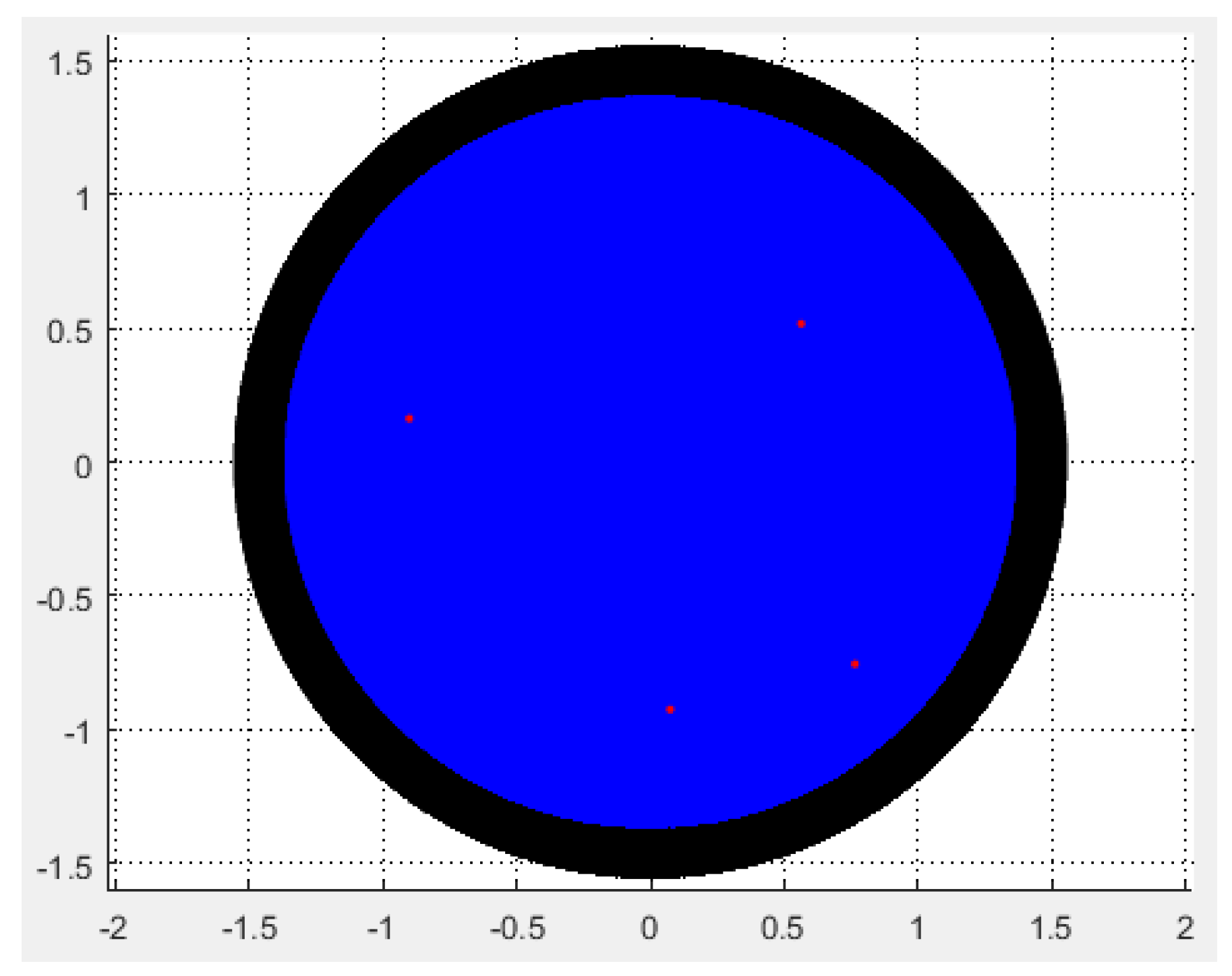
Theorem 6. Letwith , and be the Chebyshev polynomial of the second kind, and let be the largest positive solution of the the following real equation Then all the zeros of are contained in .
Proof. According to Corollary 2, the comrade matrix of the polynomial
is the matrix (
5). For a real number
0, denote
, where
is the diagonal matrix with diagonal
. By simple calculations, we have
Here,
and
have the same eigenvalues. The Brauer column set of
is the union of 2 parts:
where
It is the
n-th deleted absolute column sum of
. From [
13], We know the fact that the entire oval of Cassini
is contained in a circle whose center is 0, radius is
So the oval of Cassini is encompassed in the disk and will be tangent to it when the value of
x satisfies
Taking the
x and multiplying this equation by
yields
By Theorem 5, this equation have one positive solution. Let
be the largest positive solution of the Equation (
8), then all the zeros of
are contained in
. □
Remark 2. Any positive solution of the Equation (8) can be used to get the inclusion sets, but it is the largest one that guarantee the smallest inclusion set because is a decreasing function of x, for 0. With Theorem 6, we naturally think of making a similar transformation on
, denoting
, through calculation, We have that
And the Brauer column set of
is
where the radius of the former part
is a non-smooth function, which makes the subsequent proof relatively complicated. In order to avoid this situation, we use the relation (
1) to obtain the following theorem.
Theorem 7. Letwith , and be the Chebyshev polynomial of the first kind, and let be the largest positive solution of the following real equation Then all the zeros of are contained in .
Proof. According to the relations of the two kinds of chebyshev polynomials, the polynomial
can be expressed as
By Theorem 6, though changing the corresponding coefficients, we have all the zeros of are contained in . □
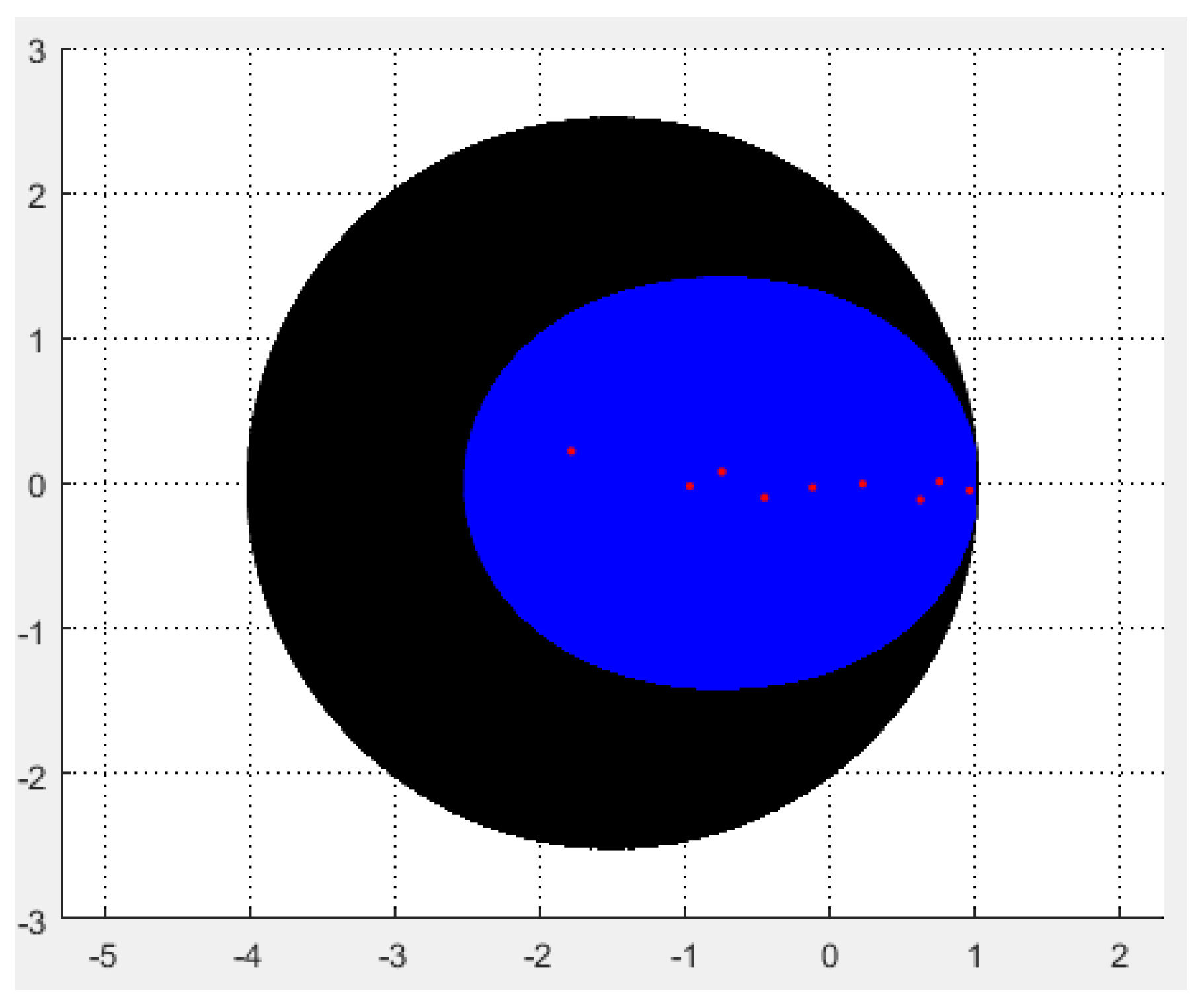
Theorem 8. Letwith , and be the Chebyshev polynomial of the second kind, and let be the largest positive solution of the following real equation Then all the zeros of are contained in Proof. In [
13], it is given that the point closest to 0 in the oval of Cassini lies at a distance given by
. Here, we take
x to make the oval of Cassini encompass the disk and be tangent to it, thus
where
is defined as in (
7). Multiplying this equation by
yields
By Theorem 5, this equation has positive roots. Let
be the largest positive solution of Equation (
9). All the zeros of
must therefore be contained in the following set
□
Theorem 9. Letwith , and is the Chebyshev polynomial of the first kind, and let be the largest positive solution of the the following real equation Then all the zeros of are contained in Proof. Similar to Theorem 7, using the relation of the two kinds of chebyshev polynomials, the polynomial
can be expressed as
According to Theorem 8, by changing the corresponding coefficients, we have the fact that all the zeros of
are contained in
□

