Turning Hild’s Sculptures into Single-Sided Surfaces


Abstract
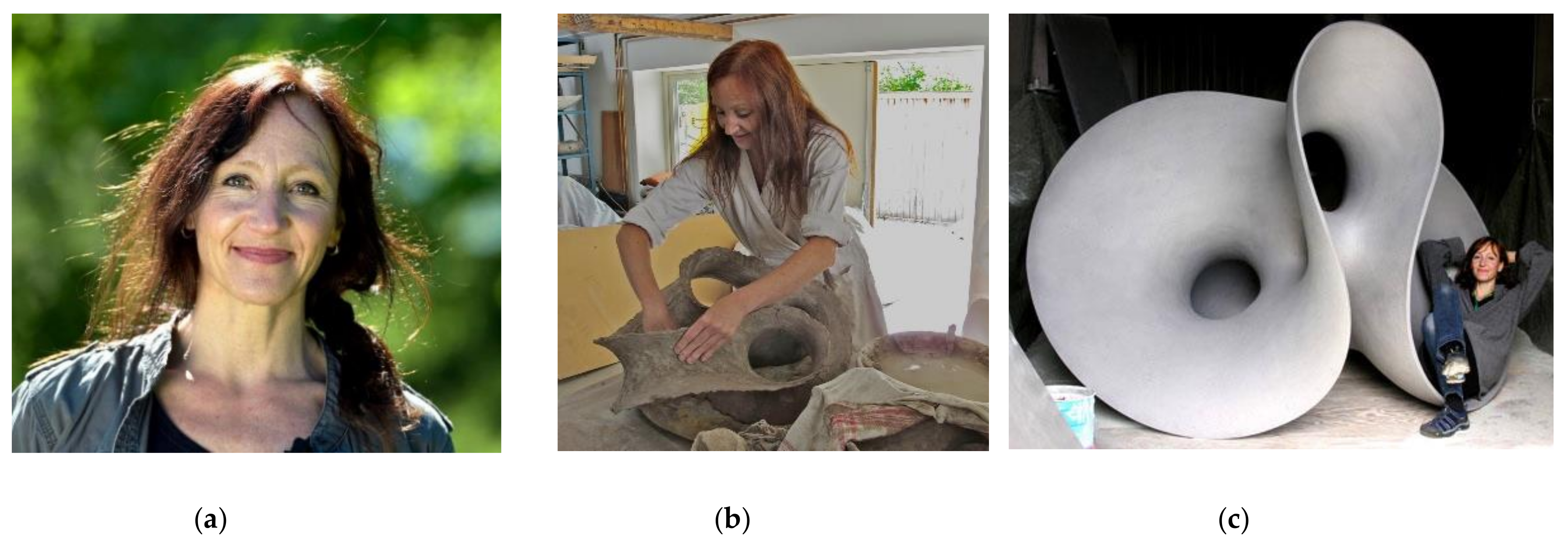
:1. Eva Hild’s Sculptures
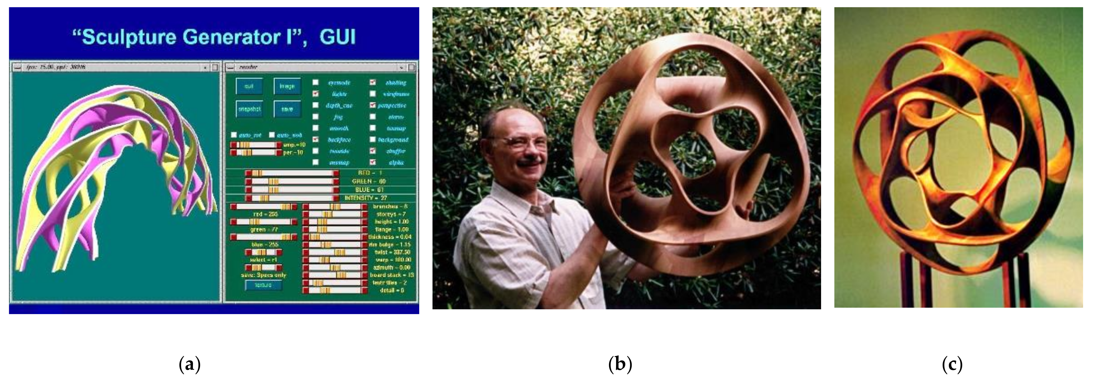
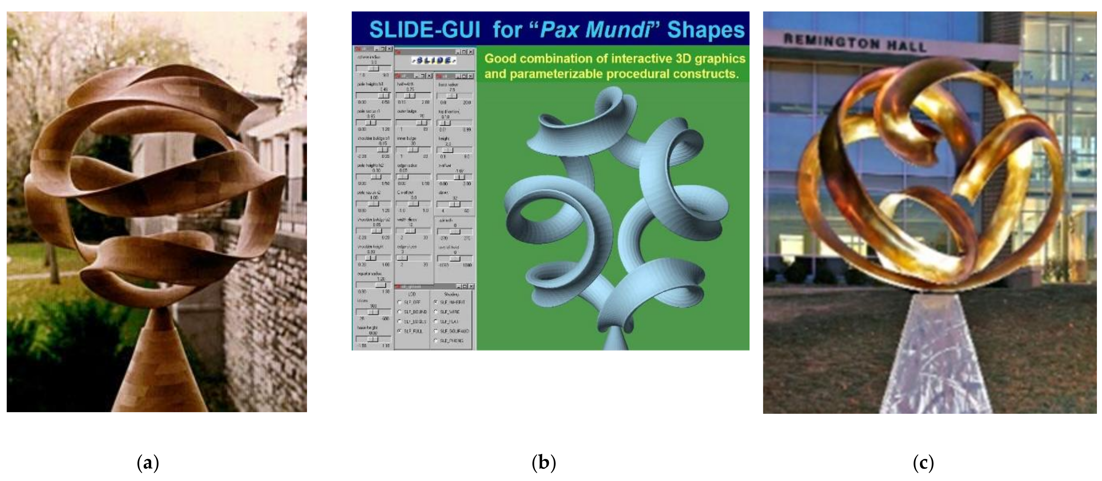
2. Background and Previous Work
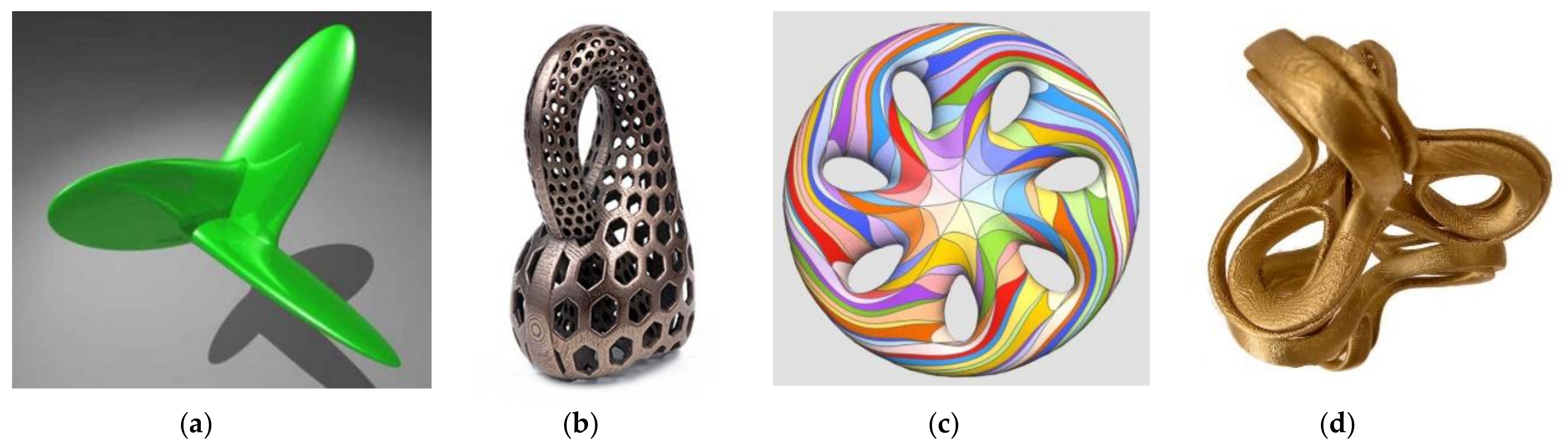
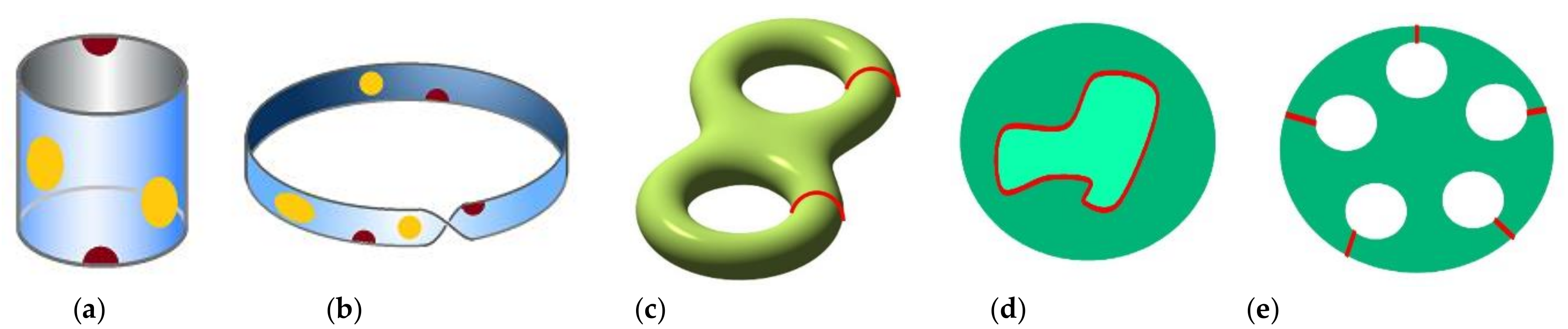
3. Classification of 2-Manifolds
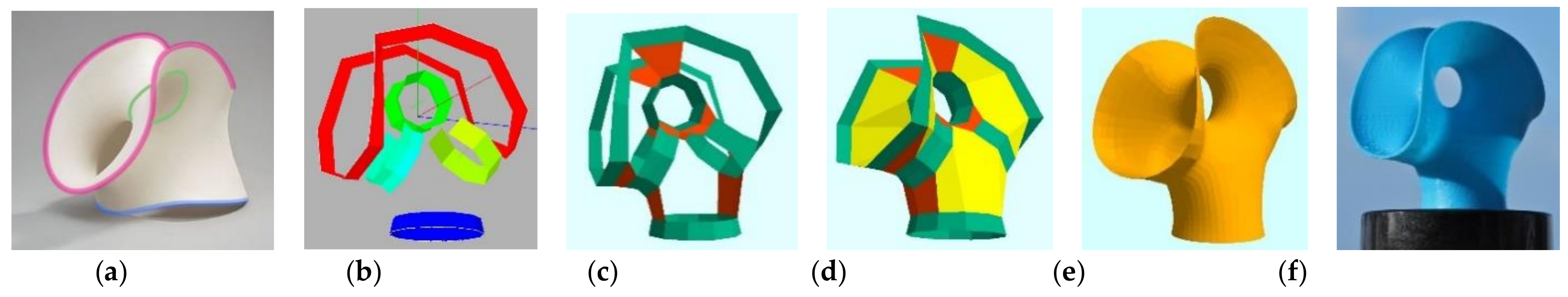
4. My Modeling Approach
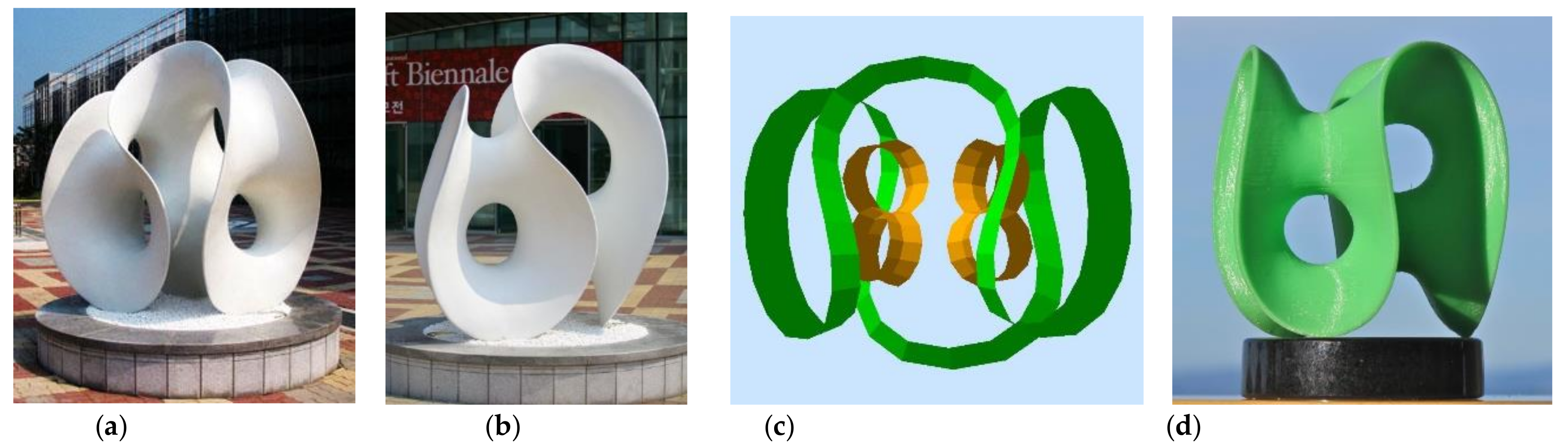
5. Modularity: Deriving New Topologies
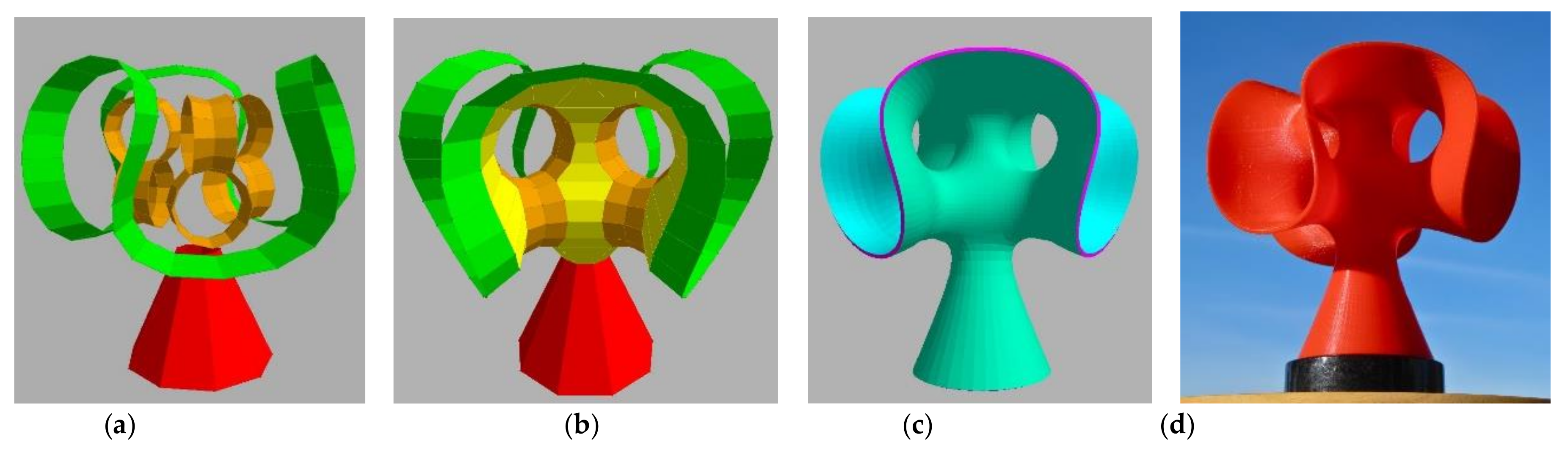
6. Wholly—A More Challenging Modeling Task
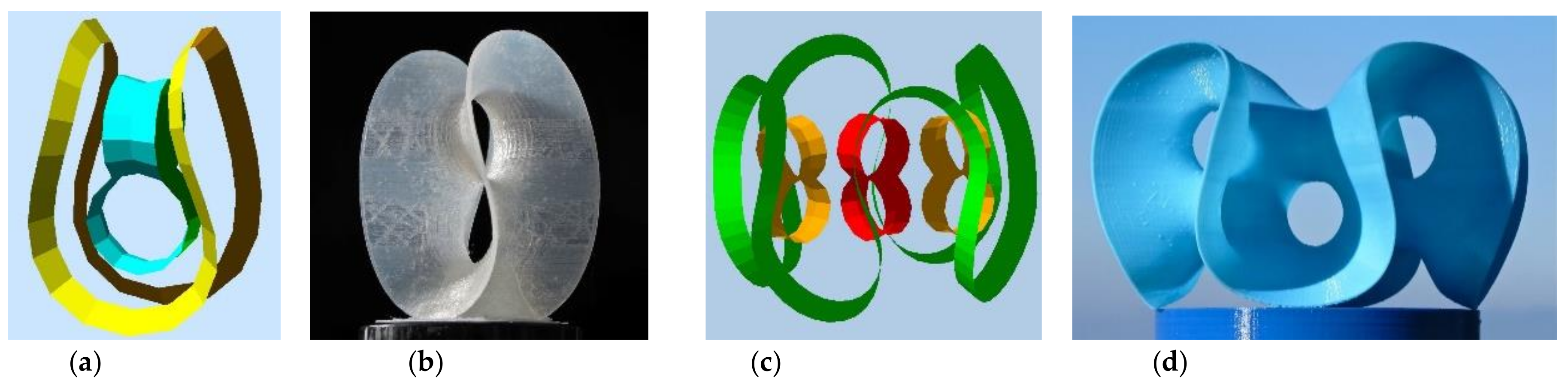
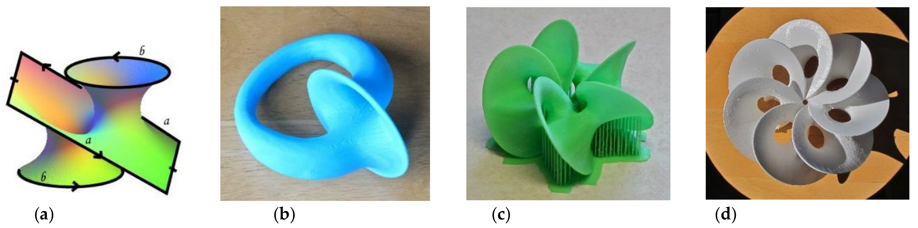
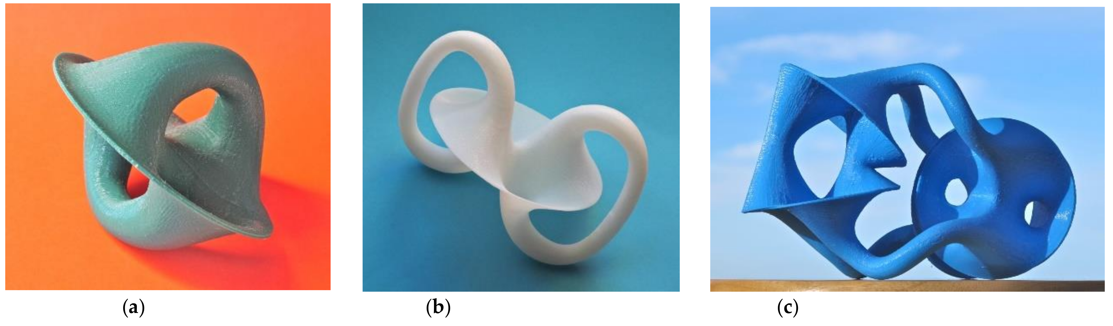
7. Introducing a Möbius Rim
8. Rings of Dyck’s Disks
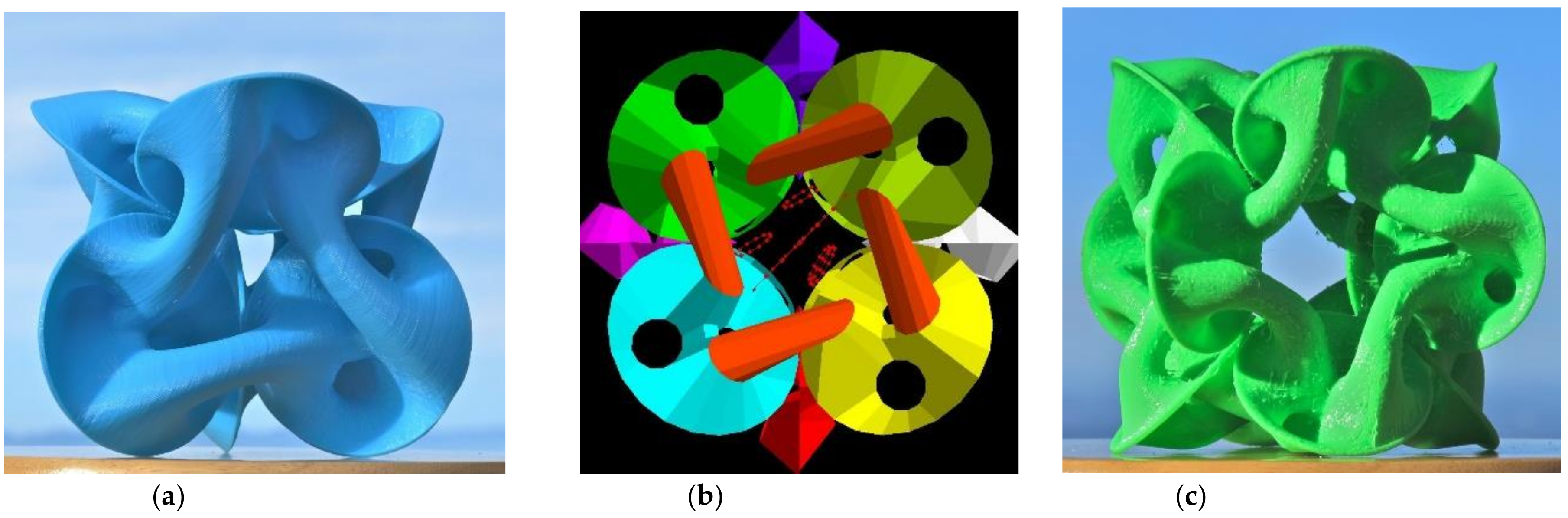
9. Dyck Clusters of Higher Genus
10. Discussion and Conclusions
Funding
Acknowledgments
Conflicts of Interest
References
- Hild, E. EVA HILD (Home Page). Available online: http://evahild.com/ (accessed on 12 January 2019).
- Friedman, N.A. Eva Hild: Topological Sculpture from Life Experience. In Proceedings of the Bridges Conference, London, UK, 4–8 August 2006; pp. 569–572. Available online: http://archive.bridgesmathart.org/2006/bridges2006-569.html (accessed on 12 January 2019).
- Friedman, N.A. Eva Hild: Sculpture and Light. Hyperseeing, August 2007; pp. 3–6. Available online: http://www.isama.org/hyperseeing/07/07-08.pdf (accessed on 12 January 2019).
- Séquin, C.H. Homage to Eva Hild. In Proceedings of the Bridges Conference, Waterloo, ON, Canada, 27–31 July 2017; pp. 117–124. Available online: http://archive.bridgesmathart.org/2017/bridges2017-117.html (accessed on 12 January 2019).
- Home of the Blender Project. Available online: https://www.blender.org/ (accessed on 12 January 2019).
- Maya, Computer Animation & Modeling Software. Available online: https://www.autodesk.com/products/maya/overview (accessed on 12 January 2019).
- Séquin, C.H. Creative Geometric Modeling with UNIGRAFIX. UCB Technical Report No. UCB/CSD-83-162, December 1983. Available online: http://www2.eecs.berkeley.edu/Pubs/TechRpts/1983/CSD-83-162.pdf (accessed on 12 January 2019).
- Collins, B. Sculpture Pictures. Bridges Virtual Museum. Available online: http://bridgesmathart.org/bcollins/bcollins.html (accessed on 12 January 2019).
- Francis, G.K. On Knot-Spanning Surfaces: An Illustrated Essay on Topologial Art. With an Artist’s Statement by Brent Collins. Leonardo J. 1992, 25, 313–320. [Google Scholar] [CrossRef]
- Séquin, C.H. Virtual Prototyping of Scherk-Collins Saddle Rings. Leonardo J. 1997, 30, 89–96. Available online: https://muse.jhu.edu/article/607427/pdf (accessed on 12 January 2019). [CrossRef]
- Séquin, C.H. Sculpture Design. In Proceedings of the 7th International Conference on Virtual Systems and Multimedia (VSMM’01), Washington, DC, USA, 25–27 October 2001; Available online: http://people.eecs.berkeley.edu/~sequin/PAPERS/VSMM01_Sculpt.pdf (accessed on 12 January 2019).
- Séquin, C.H. Part Description and Specifications for “Heptagonal Toroid”. Available online: https://people.eecs.berkeley.edu/~sequin/SFF/spec.heptoroid.html (accessed on 12 January 2019).
- Scherk’s Second Minimal Surface. Wikipedia. Available online: https://en.wikipedia.org/wiki/Scherk_surface#/media/File:Scherk%27s_second_surface.png (accessed on 12 January 2019).
- Séquin, C.H. Part Description and Specifications for “Pax Mundi”. Available online: https://people.eecs.berkeley.edu/~sequin/SCULPTS/CHS_bronzes/paxmundi.html (accessed on 12 January 2019).
- Smith, J. SLIDE Design Environment. 2003. Available online: http://www.cs.berkeley.edu/~ug/slide/ (accessed on 12 January 2019).
- Séquin, C.H. Viae Globi—Pathways on a Sphere. Proceedings M+D 2001, Geelong, Australia, July 2001. Available online: http://people.eecs.berkeley.edu/~sequin/PAPERS/MD2001_ViaeGlobi.pdf (accessed on 12 January 2019).
- Reinmuth, S. Reinmuth Bronze Studio, Inc. Available online: http://www.reinmuth.com/ (accessed on 12 January 2019).
- Séquin, C.H. Art, Geometry, and Abstract Sculpture, Figure 1, PAX MUNDI. Available online: https://www2.eecs.berkeley.edu/Research/Projects/Data/270.html (accessed on 12 January 2019).
- Séquin, C.H. The Beauty of Knots, Figure 5b, Collins’ “Music of the Spheres” (with Steve Reinmuth and Brent Collins). Available online: https://people.eecs.berkeley.edu/~sequin/CS39/TEXT/BeautyOfKnots.pdf (accessed on 12 January 2019).
- Ferguson, C. Helaman Ferguson: Mathematics in Stone and Bronze; Meridian Creative Group: Erie, PA, USA, 1994. [Google Scholar]
- Ferguson, H. Topological Design of Sculptured Surfaces. Comput. Graph. 1992, 26, 149–156. Available online: http://papers.cumincad.org/data/works/att/2b7a.content.pdf (accessed on 12 January 2019). [CrossRef]
- Hart, G.W. Geometric Sculpture (Home Page). Available online: https://www.georgehart.com/sculpture/sculpture.html (accessed on 12 January 2019).
- Hart, G.W. Icosahedral Constructions. In Proceedings of the Bridges Conference, Winfield, KS, USA, 28–30 July 1998; pp. 195–202. Available online: http://archive.bridgesmathart.org/1998/bridges1998-195.pdf (accessed on 12 January 2019).
- Hart, G.W. Sculpture from Symmetrically Arranged Planar Components. In Proceedings of the Bridges Conference, Granada, Spain, 23–26 July 2003; pp. 315–322. Available online: http://archive.bridgesmathart.org/2003/bridges2003-315.html (accessed on 12 January 2019).
- Hart, G.W. Modular Kirigami. In Proceedings of the Bridges Conference, San Sebastian, Spain, 24–27 July 2007; pp. 1–8. Available online: http://archive.bridgesmathart.org/2007/bridges2007-1.html (accessed on 12 January 2019).
- Grossman, B. Bathsheba Sculpture. (Home Page). Available online: https://bathsheba.com/ (accessed on 12 January 2019).
- Bulatov, V. Bulatov Abstract Creations. (Home Page). Available online: http://bulatov.org/ (accessed on 12 January 2019).
- Roelofs, R. Sculpture. (Home Page). Available online: http://www.rinusroelofs.nl/sculpture/sculpture-00.html (accessed on 12 January 2019).
- Schepker, H. Glass Geometry. (Home Page). Available online: https://glassgeometry.com/intro.html (accessed on 12 January 2019).
- Perry, C.O. Selected Works 1964–2011; The Perry Sudio: Norwalk, CT, USA, 2011. [Google Scholar]
- Perry, C.O.; Charles, O. PERRY (Home Page). Available online: http://www.charlesperry.com/ (accessed on 12 January 2019).
- Perry, C.O. On the Edge of Science: The Role of the Scientist’s Intuition in Science. Leonardo J. 1992, 25, 249–252. [Google Scholar] [CrossRef]
- Perry, C.O. Art and the Age of the Sciences. In The Visual Mind II; Emmer, M., Ed.; MIT Press: Cambridge, MA, USA, 2005; pp. 235–252. [Google Scholar]
- Van Wijk, J.J.; Cohen, A.M. Visualization of Seifert Surfaces. IEEE Trans. Vis. Comput. Graph. 2006, 12, 485–496. Available online: https://ieeexplore.ieee.org/abstract/document/1634314 (accessed on 12 January 2019). [CrossRef] [PubMed]
- Van Wijk, J.J. Seifertview. Available online: http://www.win.tue.nl/~vanwijk/seifertview/ (accessed on 12 January 2019).
- Apéry, F. Boy’s Surface (Apery). Available online: http://xahlee.info/surface/boys_apery/boys_apery.html (accessed on 12 January 2019).
- Séquin, C.H. Cross-Caps‒Boy Caps‒Boy Cups. In Proceedings of the Bridges Conference, Enschede, The Netherlands, 27–31 July 2013; pp. 207–216. Available online: http://archive.bridgesmathart.org/2013/bridges2013-207.html (accessed on 12 January 2019).
- Grossmann, B. The Klein Bottle Opener. Available online: https://bathsheba.com/math/klein/ (accessed on 12 January 2019).
- Séquin, C.H. On the Number of Klein Bottle Types. J. Math. Arts 2013, 7, 51–63. Available online: http://people.eecs.berkeley.edu/~sequin/PAPERS/2013_JMA_Klein-bottles.pdf (accessed on 12 January 2019). [CrossRef]
- Jarke, J.; van Wijk, J.J. Symmetric tiling of closed surfaces: Visualization of regular maps. ACM Trans. Graph. (TOG) 2009, 28, 49. Available online: https://dl.acm.org/citation.cfm?id=1531355 (accessed on 12 January 2019).
- Razafindrazaka, F.H.; Polthier, K. Regular Surfaces and Regular Maps. In Proceedings of the Bridges Conference, Seoul, Korea, 14–19 August 2014; pp. 225–234. Available online: http://archive.bridgesmathart.org/2014/bridges2014-225.html (accessed on 15 January 2019).
- Razafindrazaka, F.H.; Polthier, K. Realization of Regular Maps of Large Genus. In Topological and Statistical Methods for Complex Data; Springer: Berlin/Heidelberg, Germany, 2015; pp. 239–252. Available online: https://pdfs.semanticscholar.org/042d/21622fe7f4314e655b10b9f5f0e40be0f151.pdf (accessed on 15 January 2019).
- Akleman, E.; Chen, J. Regular Meshes. In Proceedings of the 2005 ACM Symposium on Solid and Physical Modeling, Cambridge, MA, USA, 13–15 June 2005; pp. 213–219. Available online: https://dl.acm.org/citation.cfm?id=1060268 (accessed on 15 January 2019).
- Akleman, E.; Chen, J. Regular Mesh Construction Algorithms Using Regular Handles. In Proceedings of the IEEE International Conference on Shape Modeling and Applications, Matsushima, Japan, 14–16 June 2006; Available online: https://ieeexplore.ieee.org/abstract/document/1631206 (accessed on 15 January 2019).
- Akleman, E.; Chen, J.; Xing, Q.; Gross, J.L. Cyclic Plain-Weaving on Polygonal Mesh Surfaces with Graph Rotation Systems. ACM Trans. Graph. (TOG) 2009, 28, 78-1–78-8. Available online: http://citeseerx.ist.psu.edu/viewdoc/download?doi=10.1.1.378.5899&rep=rep1&type=pdf (accessed on 15 January 2019). [CrossRef]
- Akleman, E.; Chen, J.; Chen, Y.L.; Xing, Q.; Gross, J.L. Cyclic Twill-Woven Objects. Comput. Graph. 2011, 35, 623–631. Available online: https://www.sciencedirect.com/science/article/pii/S0097849311000422 (accessed on 15 January 2019). [CrossRef]
- Friedman, N.A. Hyperseeing, Hypersculptures, Knots, and Minimal Surfaces. Available online: https://www.mi.sanu.ac.rs/vismath/nat/index.html (accessed on 15 January 2019).
- Séquin, C.H. Tangled Knots. In Proceedings of the “Art + Math = X” International Conference, Boulder, CO, USA, 2–5 June 2005; pp. 161–165. Available online: https://people.eecs.berkeley.edu/~sequin/PAPERS/ArtMath05_TangledKnots.pdf (accessed on 12 January 2019).
- Séquin, C.H. Splitting Tori, Knots, and Moebius Bands. In Proceedings of the Bridges Conference, Banff, AB, Canada, 31 July–3 August 2005; pp. 211–218. Available online: http://archive.bridgesmathart.org/2005/bridges2005-211.html (accessed on 15 January 2019).
- Akleman, E.; Yuksel, C. On a Family of Symmetric, Connected and High Genus Sculptures. In Proceedings of the Bridges Conference, London, UK, 4–8 August 2006; pp. 145–150. Available online: https://archive.bridgesmathart.org/2006/bridges2006-145.pdf (accessed on 15 January 2019).
- Séquin, C.H. Sculpture Designs Based on Borromean Soap Films. UCB Tech Report (EECS-2018-192), December 2018. Available online: https://www2.eecs.berkeley.edu/Pubs/TechRpts/2018/EECS-2018-192.html (accessed on 15 January 2019).
- Wikipedia. Rhinoceros 3D. Available online: https://en.wikipedia.org/wiki/Rhinoceros_3D (accessed on 15 January 2019).
- Akleman, E. TopMod—Topological Mesh Modeling. Available online: http://people.tamu.edu/~ergun/research/topology/index.html (accessed on 15 January 2019).
- Friedman, N.A.; Séquin, C.H. Keizo Ushio’s Sculptures, Split Tori and Möbius Bands. J. Math. Arts 2007, 1, 47–57. Available online: https://www.tandfonline.com/doi/abs/10.1080/17513470701217217 (accessed on 15 January 2019). [CrossRef]
- Longhurst, R. Robert Longhurst Studio. Available online: http://www.robertlonghurst.com/ (accessed on 15 January 2019).
- Wills, T. D-Forms: 3D forms from two 2D sheets. In Proceedings of the Bridges Conference, London, UK, 4–8 August 2006; pp. 503–510. Available online: https://archive.bridgesmathart.org/2006/bridges2006-503.html (accessed on 15 January 2019).
- Akgün, T.; Kaya, I.; Koman, A.; Akleman, E. Developable Sculptural Forms of Ilhan Koman. In Proceedings of the Bridges Conference, London, UK, 4–8 August 2006; pp. 343–350. Available online: http://archive.bridgesmathart.org/2006/bridges2006-343.html (accessed on 15 January 2019).
- Akgün, T.; Kaya, I.; Koman, A.; Akleman, E. Spiral Developable Sculptures of Ilhan Koman. In Proceedings of the Bridges Conference, San Sebastian, Spain, 24–27 July 2007; pp. 47–52. Available online: https://archive.bridgesmathart.org/2007/bridges2007-47.pdf (accessed on 15 January 2019).
- Séquin, C.H. 2-Manifold Sculptures. In Proceedings of the Bridges Conference, Baltimore, MD, USA, 29 July–2 August 2015; pp. 17–26. Available online: http://archive.bridgesmathart.org/2015/bridges2015-17.html (accessed on 1 January 2019).
- Hild, E. Interruption. Available online: https://www.bukowskis.com/en/auctions/H043/67-an-eva-hild-stoneware-sculpture-interruption-2002 (accessed on 1 January 2019).
- Wang, Y. Robust Geometry Kernel and UI for Handling Non-Orientable 2-Mainfolds. UCB TechReport (EECS-2016-65), 12 May 2016. Available online: https://www2.eecs.berkeley.edu/Pubs/TechRpts/2016/EECS-2016-65.html (accessed on 1 January 2019).
- Dieppedalle, G. Interactive CAD Software for the Design of Free-form 2-Manifold Surfaces. (NOME). UCB TechReport (EECS-2018-48), 10 May 2018. Available online: https://www2.eecs.berkeley.edu/Pubs/TechRpts/2018/EECS-2018-48.html (accessed on 1 January 2019).
- Catmull, E.; Clark, J. Recursively generated B-spline surfaces on arbitrary topological meshes. Comput. Aided Des. 1978, 10, 350–355. [Google Scholar] [CrossRef]
- What Is an STL File? Available online: https://www.3dsystems.com/quickparts/learning-center/what-is-stl-file (accessed on 1 January 2019).
- Séquin, C.H. Shape Representation: “Gabo Curve.” (Slide 36). Available online: http://slideplayer.com/slide/9035370/ (accessed on 1 January 2019).
- Asimov, D.; Lerner, D. Sudanese Möbius Band. Issue 17, SIGGRAPH ’84: Electronic Theater. Available online: https://search.library.brown.edu/catalog/b7650865 (accessed on 24 January 2019).
- Dyck Surface. Available online: http://www.mathcurve.com/surfaces/dyck/dyck.shtml (accessed on 12 January 2019).
- Séquin, C.H. Pentagonal Dyck Cycle. Available online: http://gallery.bridgesmathart.org/exhibitions/2017-bridges-conference/sequin (accessed on 1 January 2019).
- Séquin, C.H. Dodecahedral-Cluster of 25 Klein-Bottles. Available online: http://gallery.bridgesmathart.org/exhibitions/2018-joint-mathematics-meetings/sequin (accessed on 12 January 2019).


© 2019 by the author. Licensee MDPI, Basel, Switzerland. This article is an open access article distributed under the terms and conditions of the Creative Commons Attribution (CC BY) license (http://creativecommons.org/licenses/by/4.0/).
Share and Cite
Séquin, C.H. Turning Hild’s Sculptures into Single-Sided Surfaces. Mathematics 2019, 7, 125. https://doi.org/10.3390/math7020125
Séquin CH. Turning Hild’s Sculptures into Single-Sided Surfaces. Mathematics. 2019; 7(2):125. https://doi.org/10.3390/math7020125
Chicago/Turabian StyleSéquin, Carlo H. 2019. "Turning Hild’s Sculptures into Single-Sided Surfaces" Mathematics 7, no. 2: 125. https://doi.org/10.3390/math7020125
APA StyleSéquin, C. H. (2019). Turning Hild’s Sculptures into Single-Sided Surfaces. Mathematics, 7(2), 125. https://doi.org/10.3390/math7020125