Formulation of Pruning Maps with Rhythmic Neural Firing

Abstract

Rhythmic neural firing is thought to underlie the operation of neural function. This triggers the construction of dynamical network models to investigate how the rhythms interact with each other. Recently, an approach concerning neural path pruning has been proposed in a dynamical network system, in which critical neuronal connections are identified and adjusted according to the pruning maps, enabling neurons to produce rhythmic, oscillatory activity in simulation. Here, we construct a sort of homomorphic functions based on different rhythms of neural firing in network dynamics. Armed with the homomorphic functions, the pruning maps can be simply expressed in terms of interactive rhythms of neural firing and allow a concrete analysis of coupling operators to control network dynamics. Such formulation of pruning maps is applied to probe the consolidation of rhythmic patterns between layers of neurons in feedforward neural networks.

1. Introduction

Rhythms are ubiquitous and have been shown to play an important role in living organisms [1,2]. Lines of research on the roles of rhythms are studied, including synchronous flashing of fireflies [3], pacemaker cells of the heart [4], synchronization of pulse-coupled oscillators [5,6], synchronous neural activity propagating in scale-free networks, random networks, and cortical neural networks [7,8]. The central questions in the above research concern the origin and the control of rhythms, that is, the issue of understanding what causes the rhythms and how the rhythms interact with each other. Especially in neural network dynamics, an important issue is to probe activity-dependent plasticity of neural connections entwined with rhythms [9,10,11]. Such a kind of plasticity is claimed to be the heart of the organization of behavior [12,13,14,15].

Classic models of neural networks have achieved state-of-the-art performances in classification [16,17,18], object detection [19,20,21], and instance segmentation [22,23,24]. One of the key structures involved in network architecture is convolution. Many operators used for edge detection or pattern recognition are convolved with input images to get different types of derivative measurement in the feature-extracting process. Input images are usually structural with geometric features. Thus, convolution can be applied to get features from input images, which are then processed by other parts of network architecture to determine a maximal score for outcome prediction. Here, instead of concerning the geometric feature extraction, our focus is on the neural network models receiving and reactivating with rhythms. Rhythms can be the features of inputs sending to neural works and also be the features of outputs activating by assemblies of neurons in neural networks. We search for a rule to derive operators from rhythmic firing of neurons. Such operators are acting on the adjustment of neural connections and hence can be convolved with the input rhythm to get features and to propagate features for rhythm formation.

Our point of departure comes from the decirculation process in neural network dynamics [25,26]. The decirculation process describes adaptation of network structure that is crucial for evolutionary neural networks to proceed from one circulating state to another. Two sorts of plasticity operators are derived to modify network structure for decirculation process [27]. One is to measure synchronous neural activity in a circulating state, whereas the other is to measure self-sustaining neural activity in a circulating state. They meet the neurobiological concept called Hebbian synaptic plasticity [12,13,14]. Such plasticity operation reflects an internal control in neural network dynamics, enabling neurons to produce rhythmic, oscillatory activity [27]. Recently, the concept of decirculation process has been extended to the concept of neural path pruning [28]. There, by setting the beginning and the ending of a desired flow of neural firing states, a pruning map can be conducted to indicate critical neuronal connections which have significant controllability in eliminating the flow of neural firing states. On this basis, a simulation result shows that a mobile robot guided by neural network dynamics can be exploited to change neuronal connections determined critically by neural path pruning with rewards and punishment. The mobile robot may result in a good performance of fault-tolerant behavior of tracking (adaptive matching of sensory inputs to motor outputs) [28].

Neural path pruning paves an alternative way to derive operators convolving with signals and controlling neural network dynamics. This motivates us to formulate pruning maps with rhythmic neural firing, which may induce a framework of feedforward neural networks for rhythm formation.

2. Theoretical Framework

The model description follows. Let ${\{0,1\}}^n$ be the n-dimensional state space consisting of all vectors $x=(x_1,x_2,\dots ,x_n)$, with each component $x_i$ being 0 or 1. Consider a dynamical system of n coupled neurons, which is modeled by the equation [25,26]:

$$x(t+1)=H_A(x\left(t\right),s\left(t\right)),t=0,1,\dots ,$$

(1)

where $x\left(t\right)=(x_1\left(t\right),x_2\left(t\right),\dots ,x_n\left(t\right))\in {\{0,1\}}^n$ is a vector of neural firing states at time t, with each component $x_i\left(t\right)$ representing the firing state of neuron i at time t; $A=\left(a_{ij}\right)\in M_n\left(\mathbb{R}\right)$ is a coupling weight matrix of the n coupled neurons (be they agents in a recurrent or feedforward neural network), with each entry $a_{ij}$ representing the coupling weight underlying the connection from j to i; $s\left(t\right)\subset \{1,2,\dots ,n\}$ denotes an ensemble of neurons which adjust their states at time t; and $H_A(·,s\left(t\right))$ is a transition function whose ith component is defined by

$${\left[H_A(x,s\left(t\right))\right]}_i=\mathrm{𝟙}\left(\sum _{j=1}^n{a}_{ij}{x}_j-b_i\right)\mathrm{if}i\in s\left(t\right),$$

(2)

otherwise ${\left[H_A(x,s\left(t\right))\right]}_i=x_i$, where $b_i\in \mathbb{R}$ is a firing threshold of neuron i for $i=1,2,\dots ,n$ and the function 𝟙 is the Heaviside function. Consider a flow $\mathrm{\Omega }=[x^0,x^1,\dots ,x^p]$ of neural firing states in ${\{0,1\}}^n$, where $p>1$, $x^0,x^1,\dots ,x^p\in {\{0,1\}}^n$, and $x^0\ne x^i$ for some $i\in \{1,2,\dots ,p\}$. Specifically, if $x^0=x^p$ within $\mathrm{\Omega }$, then $\mathrm{\Omega }$ is said to be a loop of neural firing states in ${\{0,1\}}^n$. For each $i,j=1,2,\dots ,n$, an integer, denoted $c_{ij}\left(\mathrm{\Omega }\right)$, is assigned according to the rule:

$$c_{ij}\left(\mathrm{\Omega }\right)=x_j^0(x_i^0-x_i^1)+x_j^1(x_i^1-x_i^2)+\cdots +x_j^{p-1}(x_i^{p-1}-x_i^p).$$

(3)

The matrix $C\left(\mathrm{\Omega }\right)=\left(c_{ij}\left(\mathrm{\Omega }\right)\right)$ is called the pruning map of $\mathrm{\Omega }$. Thus,

$$\begin{array}{ccc}\hfill C\left(\mathrm{\Omega }\right)& =& \left(\begin{array}{ccc}{\displaystyle \sum _{m=1}^p{x}_1^{m-1}(x_1^{m-1}-x_1^m)}& \cdots & {\displaystyle \sum _{m=1}^p{x}_n^{m-1}(x_1^{m-1}-x_1^m)}\\ ⋮& \ddots & ⋮\\ {\displaystyle \sum _{m=1}^p{x}_1^{m-1}(x_n^{m-1}-x_n^m)}& \cdots & {\displaystyle \sum _{m=1}^p{x}_n^{m-1}(x_n^{m-1}-x_n^m)}\end{array}\right).\hfill \end{array}$$

(4)

The pruning map $C\left(\mathrm{\Omega }\right)$ induces the linear functional $A⟶⟨A,C\left(\mathrm{\Omega }\right)⟩$, which is defined on the Hilbert space $M_n\left(\mathbb{R}\right)$ of all real $n\times n$ matrices endowed with the Hilbert–Schmidt inner product $⟨·,·⟩$, where $⟨A,C\left(\mathrm{\Omega }\right)⟩={\sum }_{i,j}{a}_{ij}{c}_{ij}\left(\mathrm{\Omega }\right)$ for each $A=\left(a_{ij}\right)\in M_n\left(\mathbb{R}\right)$. Let $⟨x,y⟩$ be the usual inner product of x and y in ${\mathbb{R}}^n$. With these notions, a basic theorem reveals the determination of whether the neural connections identified by the pruning map are crucial to eliminate the flow of neural firing states in the dynamics of the neural network. It was stated in [27,28] as follows.

Theorem 1.

Let $\mathrm{\Omega }=[x^0,x^1,\dots ,x^p]$ be a flow of neural firing states in ${\{0,1\}}^n$. If $A\in M_n\left(\mathbb{R}\right)$ and $b\in {\mathbb{R}}^n$ satisfy

$$⟨A,C\left(\mathrm{\Omega }\right)⟩>⟨b,x^0-x^p⟩,$$

(5)

then for any initial neural firing state $x\left(0\right)\in {\{0,1\}}^n$ and any updating $s\left(t\right)\subset \{1,2,\dots ,n\}$, $t=0,1,\dots ,$ the flow $x\left(t\right)$ encoded by Equation (1) cannot behave in

$$x\left(T\right)=x^0,x(T+1)=x^1,\dots ,x(T+p)=x^p$$

(6)

for each $T=0,1,\dots .$

Theorem 1 is based on the concept of neural path pruning. It points out a regulatory regime for network formation. To show this, consider a flow $\mathrm{\Omega }=[x^0,x^1,\dots ,$$x^p]$ and a coupling weight matrix $A=\left(a_{ij}\right)\in M_n\left(\mathbb{R}\right)$. If we choose a coupling operator $D=\left(d_{ij}\right)\in M_n\left(\mathbb{R}\right)$ such that $⟨D,C\left(\mathrm{\Omega }\right)⟩\ge 0$ (respectively, $⟨D,C\left(\mathrm{\Omega }\right)⟩\le 0$), then

$$\begin{array}{cc}⟨A+D,C\left(\mathrm{\Omega }\right)⟩\ge ⟨A,C\left(\mathrm{\Omega }\right)⟩& \hfill \end{array}$$

(7)

$$\begin{array}{cc}(resp.,⟨A+D,C(\mathrm{\Omega })⟩\le ⟨A,C(\mathrm{\Omega })⟩).& \hfill \end{array}$$

(8)

Since the quantity $⟨b,x^0-x^p⟩$ is determined only by the flow $\mathrm{\Omega }$ and the threshold b, Theorem 1 coupled with the inequality in Equation (7) (respectively, the inequality in Equation (8)) suggests that, given the dynamical system

$$x(t+1)=H_{A+D}(x\left(t\right),s\left(t\right)),t=0,1,\dots ,$$

(9)

the change of the coupling weight matrix from A to $A+D$ may enhance (respectively, inhibit) the effect of flow elimination on $\mathrm{\Omega }$.

We go further to probe the pruning map with a desired flow of rhythmic neural firing. Each entry in the pruning map may be represented in terms of a quantity related to the firing rhythms of individual neurons. In so doing, we can directly extract information from the pruning map concerning how the rhythms interact with each other. Specifically, for feedforward neural networks, the pruning map provides a recipe to probe the interaction of rhythms between layers, which may reveal a consolidated rule to keep neurons firing in their specific rhythms consistently.

3. Main Results

Assume that neuron i fires in rhythm $r_i\in \mathbb{N}$ for $i=1,2,\dots ,n.$ Let $p=\mathrm{l}\mathrm{c}\mathrm{m}(r_1,r_2,\dots ,r_n)$, where $\mathrm{l}\mathrm{c}\mathrm{m}(r_1,r_2,\dots ,r_n)$ denotes the least common multiple of $r_1,r_2,\dots ,r_n$. For each $i=1,2,\dots ,n$, let $m_i$ be a nonnegative integer less than $r_i$, denoting the initial phase of rhythmic neural firing. Thus, the flow with neurons firing in rhythm $r_1,r_2,\dots ,r_n$ and in phase $m_1,m_2,\dots ,m_n$ can be described as

$$\mathrm{\Omega }=[x^0,x^1,\dots ,x^p],$$

(10)

where $x_i^m=1$ if $m=m_i+k{r}_i$ for $k=0,1,\dots ,\lfloor (p-m_i)/r_i\rfloor$ and $i=1,2,\dots ,n$; otherwise, $x_i^m=0$. Here, the notation $\lfloor r\rfloor$ denotes the largest integer less than or equal to $r\in \mathbb{R}$. Theorem 2 represents a matrix decomposition formula of the pruning map underlying rhythmic neural firing.

Theorem 2.

Let $\mathrm{\Omega }=[x^0,x^1,\dots ,x^p]$ be a flow of rhythmic neural firing states given in Equation (10). For each $i,j=1,2,\dots ,n,$ denote by $lcm(r_i,r_j)$ the least common multiple of $r_i$ and $r_j$, and $gcd(r_i,r_j)$ the greatest common divisor of $r_i$ and $r_j$. Let ${\left[m_i\right]}_{gcd(r_i,r_j)}$ denote the nonnegative integer less than $gcd(r_i,r_j)$ such that

$${\left[m_i\right]}_{gcd(r_i,r_j)}\equiv m_{i}modgcd(r_i,r_j).$$

(11)

Then, the pruning map $C\left(\mathrm{\Omega }\right)$ can be formulated by $C\left(\mathrm{\Omega }\right)=\widehat{C}\left(\mathrm{\Omega }\right)+C^{♮}\left(\mathrm{\Omega }\right),$ where $\widehat{C}\left(\mathrm{\Omega }\right)=\left({\widehat{c}}_{ij}\left(\mathrm{\Omega }\right)\right)$ is a symmetric matrix whose non-zero entries are given by

$$\begin{array}{cc}\hfill {\widehat{c}}_{ij}\left(\mathrm{\Omega }\right)={\widehat{c}}_{ji}\left(\mathrm{\Omega }\right)=-p/lcm(r_i,r_j)& if gcd(r_i,r_j)=2and{[m_j+1]}_{gcd(r_i,r_j)}={\left[m_i\right]}_{gcd(r_i,r_j)},\hfill \end{array}$$

(12)

$$\begin{array}{cc}\hfill {\widehat{c}}_{ij}\left(\mathrm{\Omega }\right)={\widehat{c}}_{ji}\left(\mathrm{\Omega }\right)=p/lcm(r_i,r_j)& if gcd(r_i,r_j)=2and{\left[m_j\right]}_{gcd(r_i,r_j)}={\left[m_i\right]}_{gcd(r_i,r_j)},\hfill \end{array}$$

(13)

and $C^{♮}\left(\mathrm{\Omega }\right)=\left(c_{ij}^{♮}\left(\mathrm{\Omega }\right)\right)$ is a non-symmetric matrix whose non-zero entries are given by

$$\begin{array}{cc}\hfill c_{ij}^{♮}\left(\mathrm{\Omega }\right)=-p/lcm(r_i,r_j)& if gcd(r_i,r_j)>2and{[m_j+1]}_{gcd(r_i,r_j)}={\left[m_i\right]}_{gcd(r_i,r_j)},\hfill \end{array}$$

(14)

$$\begin{array}{cc}\hfill c_{ij}^{♮}\left(\mathrm{\Omega }\right)=c_{ji}^{♮}\left(\mathrm{\Omega }\right)=p/lcm(r_i,r_j)& if gcd(r_i,r_j)>2and{\left[m_j\right]}_{gcd(r_i,r_j)}={\left[m_i\right]}_{gcd(r_i,r_j)}.\hfill \end{array}$$

(15)

Proof. 

To prove Theorem 2, note that if $m_j>0$, then $1\ne r_j>m_j>0$ and

$$(\mathrm{l}\mathrm{c}\mathrm{m}(r_1,r_2,\dots ,r_n)-1)/r_j\ge (p-m_j)/r_j\ge (\mathrm{l}\mathrm{c}\mathrm{m}(r_1,r_2,\dots ,r_n)-r_j+1)/r_j.$$

(16)

Thus, we have

$$\lfloor (p-m_j)/r_j\rfloor =\left\{\begin{array}{ccc}\mathrm{l}\mathrm{c}\mathrm{m}(r_1,r_2,\dots ,r_n)/r_j-1\hfill & \mathrm{if}& m_j\ne 0,\\ \mathrm{l}\mathrm{c}\mathrm{m}(r_1,r_2,\dots ,r_n)/r_j\hfill & \mathrm{if}& m_j=0.\end{array}\right.$$

(17)

Denote by $k_j=\mathrm{l}\mathrm{c}\mathrm{m}(r_1,r_2,\dots ,r_n)/r_j-1$ for $j=1,2,\dots ,n$. Since $x_j^m=1$ if and only if $m=m_j+k{r}_j$ for $k=0,1,\dots ,\lfloor (p-m_j)/r_j\rfloor$, the $ij$-entry of the pruning map $C\left(\mathrm{\Omega }\right)$ is reduced by

$$\begin{array}{cc}{c}_{ij}\left(\mathrm{\Omega }\right)\hfill & ={\displaystyle \sum _{m=1}^p}{x}_j^{m-1}\left(x_i^{m-1}-x_i^m\right)\hfill \\ & ={\displaystyle \sum _{k=0}^{k_j}}{x}_j^{m_j+k{r}_j}\left(x_i^{m_j+k{r}_j}-x_i^{m_j+k{r}_j+1}\right)\hfill \\ & ={\displaystyle \sum _{k=0}^{k_j}}\left(x_i^{m_j+k{r}_j}-x_i^{m_j+k{r}_j+1}\right).\hfill \end{array}$$

(18)

To compute Equation (18) for each pair of $i,j=1,2,\dots ,n$, we estimate the numbers of elements in the intersections

$$\left\{m_j+k{r}_j;k=0,1,\dots ,k_j\right\}\bigcap \{m_i+k{r}_i;k=0,1,\dots ,\lfloor (p-m_i)/r_i\rfloor \}$$

(19)

and

$$\left\{m_j+k{r}_j+1;k=0,1,\dots ,k_j\right\}\bigcap \{m_i+k{r}_i;k=0,1,\dots ,\lfloor (p-m_i)/r_i\rfloor \}.$$

(20)

Denote by $g_{ij}=gcd(r_i,r_j)$. Consider the spanning class ${⟨a⟩}_{r_i}$ (respectively, ${⟨a⟩}_{g_{ij}}$) consisting of all $a+k{r}_i$ (respectively, $a+k{g}_{ij}$), where k runs through all the integers. Let

$${\mathbb{Z}}_{r_i}=\{{⟨0⟩}_{r_i},{⟨1⟩}_{r_i},\dots ,{⟨r_i-1⟩}_{r_i}\}$$

(21)

and

$${\mathbb{Z}}_{g_{ij}}=\{{⟨0⟩}_{g_{ij}},{⟨1⟩}_{g_{ij}},\dots ,{⟨g_{ij}-1⟩}_{g_{ij}}\}.$$

(22)

Define the mapping $\mathrm{\Psi }:{\mathbb{Z}}_{r_i}⟶{\mathbb{Z}}_{g_{ij}}$ by

$$\mathrm{\Psi }\left({⟨a⟩}_{r_i}\right)={⟨a⟩}_{g_{ij}}.$$

(23)

Then, $\mathrm{\Psi }$ is a homomorphism of ${\mathbb{Z}}_{r_i}$ onto ${\mathbb{Z}}_{g_{ij}}$. We claim that the kernel of $\mathrm{\Psi }$, denoted by $\mathrm{K}\mathrm{e}\mathrm{r}\mathrm{\Psi }$, is

$$\mathrm{K}\mathrm{e}\mathrm{r}\mathrm{\Psi }=\left\{{⟨k{r}_j⟩}_{r_i};k\in \mathbb{Z}\right\}.$$

(24)

It is readily seen that $k{r}_j\equiv 0mod{g}_{ij}$ for each $k\in \mathbb{Z}$, so ${⟨k{r}_j⟩}_{g_{ij}}={⟨0⟩}_{g_{ij}}$, which implies that

$$\mathrm{K}\mathrm{e}\mathrm{r}\mathrm{\Psi }\supset \left\{{⟨k{r}_j⟩}_{r_i};k\in \mathbb{Z}\right\}.$$

(25)

On the other hand, suppose ${⟨a⟩}_{r_i}\in \mathrm{K}\mathrm{e}\mathrm{r}\mathrm{\Psi }$. Then, $a=\delta g_{ij}$ for some $\delta \in \mathbb{Z}$. Since $g_{ij}$ is the greatest common divisor of $r_i$ and $r_j$, there exist $\alpha ,\beta \in \mathbb{Z}$ such that

$$g_{ij}=\alpha r_i+\beta r_j.$$

(26)

This shows that

$$a=\delta \alpha r_i+\delta \beta r_j,$$

(27)

and hence $a\equiv \delta \beta r_{j}mod{r}_i$, proving the Equation (24). Thus, ${\mathbb{Z}}_{r_i}/\left\{{⟨k{r}_j⟩}_{r_i};k\in \mathbb{Z}\right\}$ is isomorphic to ${\mathbb{Z}}_{g_{ij}}$. Denote by $l_{ij}=lcm(r_i,r_j)$. Since

$$l_{ij}=(r_i{r}_j/g_{ij})|p$$

(28)

and the order of the kernel of $\mathrm{\Psi }$ is $\left|\mathrm{Ker}\mathrm{\Psi }\right|=|{\mathbb{Z}}_{r_i}|/|{\mathbb{Z}}_{g_{ij}}|=r_i/g_{ij}$, we may explicitly rewritten $\mathrm{K}\mathrm{e}\mathrm{r}\mathrm{\Psi }$ by

$$\begin{array}{cc}\hfill \mathrm{K}\mathrm{e}\mathrm{r}\mathrm{\Psi }& =\{{⟨0⟩}_{r_i},{⟨r_j⟩}_{r_i},{⟨2r_j⟩}_{r_i},\dots ,{⟨(r_i/g_{ij}-1)r_j⟩}_{r_i}\}\hfill \\ & =\{{⟨l_{ij}⟩}_{r_i},{⟨l_{ij}+r_j⟩}_{r_i},{⟨l_{ij}+2r_j⟩}_{r_i},\dots ,{⟨l_{ij}+(r_i/g_{ij}-1)r_j⟩}_{r_i}\}\hfill \\ & =\cdots \hfill \\ & =\left\{{⟨p-l_{ij}⟩}_{r_i},{⟨p-l_{ij}+r_j⟩}_{r_i},{⟨p-l_{ij}+2r_j⟩}_{r_i},\dots ,{⟨p-l_{ij}+(r_i/g_{ij}-1)r_j⟩}_{r_i}\right\}.\hfill \end{array}$$

(29)

On the other hand, since

$$\mathrm{K}\mathrm{e}\mathrm{r}\mathrm{\Psi }=\{{⟨0⟩}_{r_i},{⟨g_{ij}⟩}_{r_i},{⟨2g_{ij}⟩}_{r_i},\dots ,{⟨(r_i/g_{ij}-1)g_{ij}⟩}_{r_i}\},$$

(30)

there exists a bijective mapping $\sigma$ on $\{0,1,\dots ,r_i/g_{ij}-1\}$ with $\sigma \left(0\right)=0$ such that

$${⟨h{l}_{ij}+k{r}_j⟩}_{r_i}={⟨\sigma \left(k\right)g_{ij}⟩}_{r_i}$$

(31)

for each $h=0,1,\dots ,p/l_{ij}-1$ and $k=0,1,\dots ,r_i/g_{ij}-1$. Recall that $m_j={\left[m_j\right]}_{g_{ij}}+\delta g_{ij}$ for some $\delta \in Z$. By Equation (30), we have

$${⟨m_j⟩}_{r_i}+\mathrm{K}\mathrm{e}\mathrm{r}\mathrm{\Psi }={⟨{\left[m_j\right]}_{g_{ij}}+\delta g_{ij}⟩}_{r_i}+\mathrm{K}\mathrm{e}\mathrm{r}\mathrm{\Psi }={⟨{\left[m_j\right]}_{g_{ij}}⟩}_{r_i}+\mathrm{K}\mathrm{e}\mathrm{r}\mathrm{\Psi },$$

(32)

and hence by Equation (31), we have

$${⟨m_j+h{l}_{ij}+k{r}_j⟩}_{r_i}={⟨{\left[m_j\right]}_{g_{ij}}+\sigma \left(k\right)g_{ij}⟩}_{r_i},$$

(33)

which implies that there exists $\lambda \in \mathbb{Z}$ such that

$$m_j+h{l}_{ij}+k{r}_j={\left[m_j\right]}_{g_{ij}}+\sigma \left(k\right)g_{ij}+\lambda r_i$$

(34)

for each $h=0,1,\dots ,p/l_{ij}-1$ and $k=0,1,\dots ,r_i/g_{ij}-1$. Since $h{l}_{ij}\le m_j+h{l}_{ij}+k{r}_j<(h+1)l_{ij}$ and $0\le {\left[m_j\right]}_{g_{ij}}+\sigma \left(k\right)g_{ij}<r_i$ for each $h=0,1,\dots ,p/l_{ij}-1$ and $k=0,1,\dots ,r_i/g_{ij}-1$, it follows from Equation (34) that

$$(h{l}_{ij}-r_i)/r_i<(m_j+h{l}_{ij}+k{r}_j-{\left[m_j\right]}_{g_{ij}}-\sigma \left(k\right)g_{ij})/r_i=\lambda <(h+1)l_{ij}/r_i.$$

(35)

Since $\lambda \in \mathbb{Z}$, we may rewrite Equation (35) by

$$h{l}_{ij}/r_i\le \lambda <(h+1)l_{ij}/r_i.$$

(36)

With the inequalities in Equations (34) and (36) established by the construction of $\mathrm{\Psi }$, we now proceed to compute Equations (19) and (20). Let $\tau \in \{0,1\}$. For the case of $m_i\ne 0$, since

$$\lfloor (p-m_i)/r_i\rfloor =p/r_i-1=(p/l_{ij}-1+1)l_{ij}/r_i-1,$$

(37)

we have

$$\begin{array}{cc}\hfill & \{m_i+k{r}_i;k=0,1,\dots ,\lfloor (p-m_i)/r_i\rfloor \}\hfill \\ =& {\displaystyle \bigcup _{h=0,1,\dots ,p/l_{ij}-1}}\{m_i+{\lambda }_h{r}_i;{\lambda }_h=h{l}_{ij}/r_i,h{l}_{ij}/r_i+1,\dots ,(h+1)l_{ij}/r_i-1\}.\hfill \end{array}$$

(38)

Furthermore, since

$$k_j{r}_j=p-r_j=(p/l_{ij}-1)l_{ij}+(r_i/g_{ij}-1)r_j,$$

(39)

we have

$$\begin{array}{cc}\hfill & \left\{m_j+\tau +k{r}_j;k=0,1,\dots ,k_j\right\}\hfill \\ =& {\displaystyle \bigcup _{h=0,1,\dots ,p/l_{ij}-1}}\left\{m_j+\tau +h{l}_{ij}+k{r}_j;k=0,1,\dots ,r_i/g_{ij}-1\right\}.\hfill \end{array}$$

(40)

Combining Equations (38) and (40) shows that

$$\begin{array}{c}\left\{m_j+\tau +k{r}_j;k=0,1,\dots ,k_j\right\}\bigcap \{m_i+k{r}_i;k=0,1,\dots ,\lfloor (p-m_i)/r_i\rfloor \}\hfill \\ =\left({\displaystyle \bigcup _{h=0,1,\dots ,p/l_{ij}-1}}\left\{m_j+\tau +h{l}_{ij}+k{r}_j;k=0,1,\dots ,r_i/g_{ij}-1\right\}\right)\hfill \\ \bigcap \left({\displaystyle \bigcup _{h=0,1,\dots ,p/l_{ij}-1}}\{m_i+{\lambda }_h{r}_i;{\lambda }_h=h{l}_{ij}/r_i,h{l}_{ij}/r_i+1,\dots ,(h+1)l_{ij}/r_i-1\}\right).\hfill \end{array}$$

(41)

Consider a partition of $\{\tau ,\tau +1,\dots ,\tau +p-1\}$ given by

$$\{\tau ,\tau +1,\dots ,\tau +p-1\}={\displaystyle \bigcup _{h=0,1,\dots ,p/l_{ij}-1}}\{h{l}_{ij}+\tau ,h{l}_{ij}+1+\tau ,\dots ,(h+1)l_{ij}-1+\tau \}.$$

(42)

Fix $h\in \{0,1,\dots ,p/l_{ij}-1\}$. Since

$$0\le m_j\le m_j+k{r}_j\le m_j+(r_i/g_{ij}-1)r_j=m_j+l_{ij}-r_j\le l_{ij}-1$$

(43)

for each $k=0,1,\dots ,r_i/g_{ij}-1$, we have

$$\{m_j+\tau +h{l}_{ij}+k{r}_j;k=0,1,\dots ,r_i/g_{ij}-1\}\subset \{h{l}_{ij}+\tau ,h{l}_{ij}+1+\tau ,\dots ,(h+1)l_{ij}-1+\tau \}.$$

(44)

Furthermore, since

$$1+h{l}_{ij}\le m_i+h{l}_{ij}\le m_i+{\lambda }_h{r}_i\le m_i+((h+1)l_{ij}/r_i-1)r_i=m_i+(h+1)l_{ij}-r_i\le (h+1)l_{ij}-1$$

(45)

for each ${\lambda }_h=h{l}_{ij}/r_i,h{l}_{ij}/r_i+1,\dots ,(h+1)l_{ij}/r_i-1$, we have

$$\begin{array}{cc}\hfill & \{m_i+{\lambda }_h{r}_i;{\lambda }_h=h{l}_{ij}/r_i,h{l}_{ij}/r_i+1,\dots ,(h+1)l_{ij}/r_i-1\}\hfill \\ \subset & \{h{l}_{ij}+1,h{l}_{ij}+2,\dots ,(h+1)l_{ij}-1\}\hfill \\ =& \{h{l}_{ij},h{l}_{ij}+1,\dots ,(h+1)l_{ij}-1\}\cap \{h{l}_{ij}+1,h{l}_{ij}+2,\dots ,(h+1)l_{ij}\}\hfill \\ \subset & \{h{l}_{ij}+\tau ,h{l}_{ij}+1+\tau ,\dots ,(h+1)l_{ij}-1+\tau \}.\hfill \end{array}$$

(46)

By Equations (42), (44) and (46), we may rearrange the intersection of elements in Equation (41) by

$$\begin{array}{c}\left\{m_j+\tau +k{r}_j;k=0,1,\dots ,k_j\right\}\bigcap \{m_i+k{r}_i;k=0,1,\dots ,\lfloor (p-m_i)/r_i\rfloor \}\hfill \\ ={\displaystyle \bigcup _{h=0,1,\dots ,p/l_{ij}-1}}(\left\{m_j+\tau +h{l}_{ij}+k{r}_j;k=0,1,\dots ,r_i/g_{ij}-1\right\}\hfill \\ \bigcap \{m_i+{\lambda }_h{r}_i;{\lambda }_h=h{l}_{ij}/r_i,h{l}_{ij}/r_i+1,\dots ,(h+1)l_{ij}/r_i-1\}).\hfill \end{array}$$

(47)

Denote by $♯E$ the number of elements in the set E. Since $0<m_i<r_i$ and $0\le {\left[m_j\right]}_{g_{ij}}+\sigma \left(k\right)g_{ij}<r_i$ for each $k=0,1,\dots ,r_i/g_{ij}-1$, it follows from Equations (34) and (36) that

$$\begin{array}{c}♯(\left\{m_j+\tau +h{l}_{ij}+k{r}_j;k=0,1,\dots ,r_i/g_{ij}-1\right\}\hfill \\ \bigcap \{m_i+{\lambda }_h{r}_i;{\lambda }_h=h{l}_{ij}/r_i,h{l}_{ij}/r_i+1,\dots ,(h+1)l_{ij}/r_i-1\})\hfill \\ =♯\left({\displaystyle \bigcup _{k=0,1,\dots ,r_i/g_{ij}-1}}\left(\{{\left[m_j\right]}_{g_{ij}}+\tau +\sigma \left(k\right)g_{ij}\}\cap \left\{m_i\right\}\right)\right)\hfill \\ =♯\left(\{{\left[m_j\right]}_{g_{ij}}+\tau ,{\left[m_j\right]}_{g_{ij}}+\tau +g_{ij},\dots ,{\left[m_j\right]}_{g_{ij}}+\tau +r_i-g_{ij}\}\cap \left\{m_i\right\}\right)\hfill \end{array}$$

(48)

for each $h=0,1,\dots ,p/l_{ij}-1$. It is readily seen that if

$$♯\left(\{{\left[m_j\right]}_{g_{ij}}+\tau ,{\left[m_j\right]}_{g_{ij}}+\tau +g_{ij},\dots ,{\left[m_j\right]}_{g_{ij}}+\tau +r_i-g_{ij}\}\cap \left\{m_i\right\}\right)=1$$

(49)

then ${\left[m_i\right]}_{g_{ij}}={[{\left[m_j\right]}_{g_{ij}}+\tau ]}_{g_{ij}}={[m_j+\tau ]}_{g_{ij}}$. Conversely, if ${\left[m_i\right]}_{g_{ij}}={[m_j+\tau ]}_{g_{ij}}$, then $m_i={\left[m_j\right]}_{g_{ij}}+\tau +\delta g_{ij}$ for some $\delta \in Z$. When $\tau =0$, it follows that

$$0\le {\left[m_j\right]}_{g_{ij}}+\tau +\delta g_{ij}<r_i\mathrm{h}\mathrm{o}\mathrm{l}\mathrm{d}\mathrm{s} \mathrm{o}\mathrm{n}\mathrm{l}\mathrm{y} \mathrm{f}\mathrm{o}\mathrm{r}\delta =0,1,\dots ,r_i/g_{ij}-1.$$

(50)

When $\tau =1$, it follows that

$$0<{\left[m_j\right]}_{g_{ij}}+\tau +\delta g_{ij}\le r_i\mathrm{h}\mathrm{o}\mathrm{l}\mathrm{d}\mathrm{s} \mathrm{o}\mathrm{n}\mathrm{l}\mathrm{y} \mathrm{f}\mathrm{o}\mathrm{r}\delta =0,1,\dots ,r_i/g_{ij}-1.$$

(51)

Since $0<m_i<r_i$, we conclude that there exists only one $\delta \in \{0,1,\dots ,r_i/g_{ij}-1\}$ such that $m_i={\left[m_j\right]}_{g_{ij}}+\tau +\delta g_{ij}$. Hence,

$$♯\left(\{{\left[m_j\right]}_{g_{ij}}+\tau ,{\left[m_j\right]}_{g_{ij}}+\tau +g_{ij},\dots ,{\left[m_j\right]}_{g_{ij}}+\tau +r_i-g_{ij}\}\cap \left\{m_i\right\}\right)=1\mathrm{if}{\left[m_i\right]}_{g_{ij}}={[m_j+\tau ]}_{g_{ij}}.$$

(52)

Thus, the equality in Equation (48) can be rewritten by

$$\begin{array}{c}♯(\left\{m_j+\tau +h{l}_{ij}+k{r}_j;k=0,1,\dots ,r_i/g_{ij}-1\right\}\hfill \\ \bigcap \{m_i+{\lambda }_h{r}_i;{\lambda }_h=h{l}_{ij}/r_i,h{l}_{ij}/r_i+1,\dots ,(h+1)l_{ij}/r_i-1\})\hfill \\ =\left\{\begin{array}{cc}1\hfill & \mathrm{if}{\left[m_i\right]}_{g_{ij}}={[m_j+\tau ]}_{g_{ij}},\hfill \\ 0\hfill & \mathrm{otherwise}\hfill \end{array}\right.\hfill \end{array}$$

(53)

for each $h=0,1,\dots ,p/l_{ij}-1$. Combining Equations (47) and (53) gives

$$\begin{array}{cc}\hfill & ♯\left(\left\{m_j+\tau +k{r}_j;k=0,1,\dots ,k_j\right\}\bigcap \{m_i+k{r}_i;k=0,1,\dots ,\lfloor (p-m_i)/r_i\rfloor \}\right)\hfill \\ =& \left\{\begin{array}{cc}p/l_{ij}\hfill & \mathrm{if}{\left[m_i\right]}_{g_{ij}}={[m_j+\tau ]}_{g_{ij}},\hfill \\ 0\hfill & \mathrm{otherwise}\hfill \end{array}\right.\hfill \end{array}$$

(54)

for the case of $m_i\ne 0$. Now, we turn to the case of $m_i=0$. Since $\lfloor (p-m_i)/r_i\rfloor =p/r_i$ and $\tau \in \{0,1\}$, we have

$$\begin{array}{cc}\hfill & \{m_i+k{r}_i;k=0,1,\dots ,\lfloor (p-m_i)/r_i\rfloor \}\hfill \\ =& \left({\displaystyle \bigcup _{h=0,1,\dots ,p/l_{ij}-1}}\{({\lambda }_h+\tau )r_i;{\lambda }_h=h{l}_{ij}/r_i,h{l}_{ij}/r_i+1,\dots ,(h+1)l_{ij}/r_i-1\}\right)\bigcup \left\{(1-\tau )p\right\}\hfill \\ \subset & \left({\displaystyle \bigcup _{h=0,1,\dots ,p/l_{ij}-1}}\{h{l}_{ij}+\tau ,h{l}_{ij}+1+\tau ,\dots ,(h+1)l_{ij}-1+\tau \}\right)\bigcup \left\{(1-\tau )p\right\}.\hfill \end{array}$$

(55)

Since Equations (40) and (44) hold also for the case $m_i=0$, they imply that

$$\begin{array}{cc}\hfill & \left\{m_j+\tau +k{r}_j;k=0,1,\dots ,k_j\right\}\hfill \\ =& {\displaystyle \bigcup _{h=0,1,\dots ,p/l_{ij}-1}}\left\{m_j+\tau +h{l}_{ij}+k{r}_j;k=0,1,\dots ,r_i/g_{ij}-1\right\}\hfill \\ \subset & {\displaystyle \bigcup _{h=0,1,\dots ,p/l_{ij}-1}}\{h{l}_{ij}+\tau ,h{l}_{ij}+1+\tau ,\dots ,(h+1)l_{ij}-1+\tau \}.\hfill \end{array}$$

(56)

The partition in Equation (42) and the inclusions in Equations (55) and (56) together imply that

$$\begin{array}{c}\left\{m_j+\tau +k{r}_j;k=0,1,\dots ,k_j\right\}\bigcap \{m_i+k{r}_i;k=0,1,\dots ,\lfloor (p-m_i)/r_i\rfloor \}\hfill \\ ={\displaystyle \bigcup _{h=0,1,\dots ,p/l_{ij}-1}}(\left\{m_j+\tau +h{l}_{ij}+k{r}_j;k=0,1,\dots ,r_i/g_{ij}-1\right\}\hfill \\ \bigcap \{({\lambda }_h+\tau )r_i;{\lambda }_h=h{l}_{ij}/r_i,h{l}_{ij}/r_i+1,\dots ,(h+1)l_{ij}/r_i-1\}).\hfill \end{array}$$

(57)

Fix $h\in \{0,1,\dots ,p/l_{ij}-1\}$. Since $\tau r_i\in \{0,r_i\}$ and $0\le {\left[m_j\right]}_{g_{ij}}+\sigma \left(k\right)g_{ij}<r_i$ for each $k=0,1,\dots ,$$r_i/g_{ij}-1$, it follows from Equations (34) and (36) that

$$\begin{array}{c}♯(\left\{m_j+\tau +h{l}_{ij}+k{r}_j;k=0,1,\dots ,r_i/g_{ij}-1\right\}\hfill \\ \bigcap \{({\lambda }_h+\tau )r_i;{\lambda }_h=h{l}_{ij}/r_i,h{l}_{ij}/r_i+1,\dots ,(h+1)l_{ij}/r_i-1\})\hfill \\ =♯\left({\displaystyle \bigcup _{k=0,1,\dots ,r_i/g_{ij}-1}}\left(\{{\left[m_j\right]}_{g_{ij}}+\tau +\sigma \left(k\right)g_{ij}\}\cap \left\{\tau r_i\right\}\right)\right)\hfill \\ =♯\left(\{{\left[m_j\right]}_{g_{ij}}+\tau ,{\left[m_j\right]}_{g_{ij}}+\tau +g_{ij},\dots ,{\left[m_j\right]}_{g_{ij}}+\tau +r_i-g_{ij}\}\cap \left\{\tau r_i\right\}\right).\hfill \end{array}$$

(58)

It is readily seen that if

$$♯\left(\{{\left[m_j\right]}_{g_{ij}}+\tau ,{\left[m_j\right]}_{g_{ij}}+\tau +g_{ij},\dots ,{\left[m_j\right]}_{g_{ij}}+\tau +r_i-g_{ij}\}\cap \left\{\tau r_i\right\}\right)=1$$

(59)

then ${[m_j+\tau ]}_{g_{ij}}={[{\left[m_j\right]}_{g_{ij}}+\tau ]}_{g_{ij}}={\left[\tau r_i\right]}_{g_{ij}}=0$. Conversely, if ${[m_j+\tau ]}_{g_{ij}}=0$, then ${\left[m_j\right]}_{g_{ij}}+\tau =\delta g_{ij}$ for some $\delta \in Z$. When $\tau =0$, it follows that

$$0\le {\left[m_j\right]}_{g_{ij}}=\delta g_{ij}<g_{ij}\mathrm{h}\mathrm{o}\mathrm{l}\mathrm{d}\mathrm{s} \mathrm{o}\mathrm{n}\mathrm{l}\mathrm{y} \mathrm{f}\mathrm{o}\mathrm{r}\delta =0.$$

(60)

When $\tau =1$, it follows that

$$0<{\left[m_j\right]}_{g_{ij}}+1=\delta g_{ij}\le g_{ij}\mathrm{h}\mathrm{o}\mathrm{l}\mathrm{d}\mathrm{s} \mathrm{o}\mathrm{n}\mathrm{l}\mathrm{y} \mathrm{f}\mathrm{o}\mathrm{r}\delta =1.$$

(61)

This implies that ${\left[m_j\right]}_{g_{ij}}+\tau =\tau g_{ij}$. Hence,

$$\begin{array}{c}♯\left(\{{\left[m_j\right]}_{g_{ij}}+\tau ,{\left[m_j\right]}_{g_{ij}}+\tau +g_{ij},\dots ,{\left[m_j\right]}_{g_{ij}}+\tau +r_i-g_{ij}\}\cap \left\{\tau r_i\right\}\right)\hfill \\ =♯\left(\{\tau g_{ij},(\tau +1)g_{ij},\dots ,r_i+(\tau -1)g_{ij}\}\cap \left\{\tau r_i\right\}\right)\hfill \\ =1\mathrm{if}{[m_j+\tau ]}_{g_{ij}}=0.\hfill \end{array}$$

(62)

Thus, the equality in Equation (58) can be rewritten by

$$\begin{array}{c}♯(\left\{m_j+\tau +h{l}_{ij}+k{r}_j;k=0,1,\dots ,r_i/g_{ij}-1\right\}\hfill \\ \bigcap \{({\lambda }_h+\tau )r_i;{\lambda }_h=h{l}_{ij}/r_i,h{l}_{ij}/r_i+1,\dots ,(h+1)l_{ij}/r_i-1\})\hfill \\ =\left\{\begin{array}{cc}1\hfill & \mathrm{if}{[m_j+\tau ]}_{g_{ij}}=0,\hfill \\ 0\hfill & \mathrm{otherwise}.\hfill \end{array}\right.\hfill \end{array}$$

(63)

Combining Equations (57) and (63) gives

$$\begin{array}{cc}\hfill & ♯\left(\left\{m_j+\tau +k{r}_j;k=0,1,\dots ,k_j\right\}\bigcap \{m_i+k{r}_i;k=0,1,\dots ,\lfloor (p-m_i)/r_i\rfloor \}\right)\hfill \\ =& \left\{\begin{array}{cc}p/l_{ij}\hfill & \mathrm{if}{\left[m_i\right]}_{g_{ij}}={[m_j+\tau ]}_{g_{ij}},\hfill \\ 0\hfill & \mathrm{otherwise}\hfill \end{array}\right.\hfill \end{array}$$

(64)

for the case of $m_i=0$. Now, we split the argument into three cases.

Case 1.$g_{ij}=1$. Then

$${\left[m_j\right]}_{g_{ij}}={[m_j+1]}_{g_{ij}}={[m_i+1]}_{g_{ij}}={\left[m_i\right]}_{g_{ij}}.$$

(65)

By Equations (18), (19), (20), (54), and (64), we have

$$c_{ij}\left(\mathrm{\Omega }\right)=c_{ji}\left(\mathrm{\Omega }\right)=p/l_{ij}-p/l_{ij}=0.$$

(66)

Case 2.$g_{ij}=2$. Then, exactly one of the following situations holds:

$${\left[m_j\right]}_{g_{ij}}={\left[m_i\right]}_{g_{ij}}or{[m_j+1]}_{g_{ij}}={\left[m_i\right]}_{g_{ij}}.$$

(67)

Suppose that ${\left[m_j\right]}_{g_{ij}}={\left[m_i\right]}_{g_{ij}}$. Then,

$${[m_j+1]}_{g_{ij}}\ne {\left[m_i\right]}_{g_{ij}}and{[m_i+1]}_{g_{ij}}\ne {\left[m_j\right]}_{g_{ij}}.$$

(68)

By Equations (18), (19), (20), (54), and (64), we have

$$c_{ij}\left(\mathrm{\Omega }\right)=c_{ji}\left(\mathrm{\Omega }\right)=p/l_{ij}.$$

(69)

Suppose that ${[m_j+1]}_{g_{ij}}={\left[m_i\right]}_{g_{ij}}$. Then,

$${\left[m_j\right]}_{g_{ij}}\ne {\left[m_i\right]}_{g_{ij}}and{[m_i+1]}_{g_{ij}}={\left[m_j\right]}_{g_{ij}}.$$

(70)

By Equations (18), (19), (20), (54), and (64), we have

$$c_{ij}\left(\mathrm{\Omega }\right)=c_{ji}\left(\mathrm{\Omega }\right)=-p/l_{ij}.$$

(71)

Case 3.$g_{ij}>2$. Suppose that ${\left[m_j\right]}_{g_{ij}}={\left[m_i\right]}_{g_{ij}}$. Then,

$${[m_j+1]}_{g_{ij}}\ne {\left[m_i\right]}_{g_{ij}}and{[m_i+1]}_{g_{ij}}\ne {\left[m_j\right]}_{g_{ij}}.$$

(72)

By Equations (18), (19), (20), (54), and (64), we have

$$c_{ij}\left(\mathrm{\Omega }\right)=c_{ji}\left(\mathrm{\Omega }\right)=p/l_{ij}.$$

(73)

Suppose that ${[m_j+1]}_{g_{ij}}={\left[m_i\right]}_{g_{ij}}$. Then,

$${\left[m_j\right]}_{g_{ij}}\ne {\left[m_i\right]}_{g_{ij}}and{[m_i+1]}_{g_{ij}}\ne {\left[m_j\right]}_{g_{ij}}.$$

(74)

By Equations (18), (19), (20), (54), and (64), we have

$$c_{ij}\left(\mathrm{\Omega }\right)=-p/l_{ij}and{c}_{ji}\left(\mathrm{\Omega }\right)=0.$$

(75)

Suppose that ${\left[m_j\right]}_{g_{ij}}\ne {\left[m_i\right]}_{g_{ij}}$ and ${[m_j+1]}_{g_{ij}}\ne {\left[m_i\right]}_{g_{ij}}$. Then, by Equations (18), (19), (20), (54), and (64), we have $c_{ij}\left(\mathrm{\Omega }\right)=0.$

This completes the proof of Theorem 2. □

As an implication, we consider a feedforward neural network consisting of many layers of neurons firing in rhythm. Suppose that there are ${\ell }_k$ neurons in layer k for each $k=1,2,\dots \overline{k}$, where layer 1 denotes the input layer and layer $\overline{k}$ denotes the output layer of the feedforward neural network. Thus, the coupling weight underlying the connection from the ℓth neuron in layer $\tilde{k}$ to the ${\ell }^{\prime }$th neuron in layer $\tilde{k}+1$ is referred to the entry $a_{ij}$, where $i={\sum }_{k=1,2,\dots ,\tilde{k}}{\ell }_k+{\ell }^{\prime }$ and $j={\sum }_{k=1,2,\dots ,\tilde{k}-1}{\ell }_k+\ell$, in the coupling weight matrix A. Thus, the coupling weight matrix A can be rewritten by

$$\left(\begin{array}{cccccccccccc}{a}_{11}& \cdots & a_{1{\ell }_1}& 0& \cdots & 0& 0& \cdots & 0& 0& \cdots & 0\\ & \ddots & & & \ddots & & & \ddots & & & \ddots & \\ a_{{\ell }_{1}1}& \cdots & a_{{\ell }_1{\ell }_1}& 0& \cdots & 0& 0& \cdots & 0& 0& \cdots & 0\\ a_{{\ell }_1+1,1}& \cdots & a_{{\ell }_1+1,{\ell }_1}& 0& \cdots & 0& 0& \cdots & 0& 0& \cdots & 0\\ & \ddots & & & \ddots & & & \ddots & & & \ddots & \\ a_{{\ell }_1+{\ell }_2,1}& \cdots & a_{{\ell }_1+{\ell }_2,{\ell }_1}& 0& \cdots & 0& 0& \cdots & 0& 0& \cdots & 0\\ 0& \cdots & 0& *& \cdots & *& 0& \cdots & 0& 0& \cdots & 0\\ & \ddots & & & \ddots & & & \ddots & & & \ddots & \\ 0& \cdots & 0& *& \cdots & *& 0& \cdots & 0& 0& \cdots & 0\\ 0& \cdots & 0& 0& \cdots & 0& a_{{\ell }_1+\cdots +{\ell }_{\overline{k}-1}+1,{\ell }_1+\cdots +{\ell }_{\overline{k}-2}+1}& \cdots & a_{{\ell }_1+\cdots +{\ell }_{\overline{k}-1}+1,{\ell }_1+\cdots +{\ell }_{\overline{k}-1}}& 0& \cdots & 0\\ & \ddots & & & \ddots & & & \ddots & & & \ddots & \\ 0& \cdots & 0& 0& \cdots & 0& a_{{\ell }_1+\cdots +{\ell }_{\overline{k}},{\ell }_1+\cdots +{\ell }_{\overline{k}-2}+1}& \cdots & a_{{\ell }_1+\cdots +{\ell }_{\overline{k}},{\ell }_1+\cdots +{\ell }_{\overline{k}-1}}& 0& \cdots & 0\end{array}\right).$$

Specifically, we may equip the input layer with a two-layer substructure, given by

$$\left(\begin{array}{ccc}{a}_{11}& \cdots & a_{1{\ell }_1}\\ & \ddots \\ a_{{\ell }_{1}1}& \cdots & a_{{\ell }_1{\ell }_1}\end{array}\right)=\left(\begin{array}{cccccc}1& 0& 0& \cdots & 0& 0\\ 1& -1& 0& \cdots & 0& 0\\ 1& 0& -1& \ddots & 0& 0\\ ⋮& ⋮& \ddots & \ddots & \ddots & ⋮\\ 1& 0& 0& \ddots & -1& 0\\ 1& 0& 0& \cdots & 0& -1\end{array}\right),$$

(76)

with the firing threshold satisfying $1>b_i>0$ for each neuron $i=1,2,\dots ,{\ell }_1$ and the updating $s\left(t\right)$ satisfying $i\in s\left(t\right)\cap s(t+1)$ if $t=m_i+\lambda r_i-1$; otherwise, $i\notin s\left(t\right)\cap s(t+1)$ for each $i=1,2,\dots ,{\ell }_1$ and $\lambda =0,1,\dots .$ Let $m_1=0$ and $r_1=1$. Then, neuron i in the input layer can fire in rhythm $r_i$ and in phase $m_i$ for each $i=1,2,\dots ,{\ell }_1$. Neurons in the posterior layer receive signals from neurons in the prior layer and fire correspondingly if the incoming signals are greater than the firing thresholds. Note that since neurons in the prior layer fire in rhythm, the firing thresholds can be adjusted to generate certain rhythmic firing patterns or combination of rhythmic firing patterns in the posterior layer. Figure 1 depicts three layers of such a feedforward neural network, in which the coupling weight matrix A is defined by

$$A=\left(\begin{array}{cccccccc}1& 0& 0& 0& 0& 0& 0& 0\\ 1& -1& 0& 0& 0& 0& 0& 0\\ 1& 0& -1& 0& 0& 0& 0& 0\\ 1& 0& 0& -1& 0& 0& 0& 0\\ 1& 0& 0& 0& -1& 0& 0& 0\\ 0& 5& 3& -1& 1& 0& 0& 0\\ 0& 1& -2& 2& 0& 0& 0& 0\\ 0& 0& 0& 0& 0& -1& 3& 0\end{array}\right),$$

(77)

the firing threshold is defined by $b=(0.5,0.5,0.5,0.5,0.5,5,2.5,2.5)$, the updating is defined initially by $s\left(0\right)=\{1,2,6,7,8\}$, and

$$\begin{array}{c}s(12\tau +1)=\{1,2,3,6,7,8\},s(12\tau +2)=\{1,3,4,6,7,8\},s(12\tau +3)=\{1,2,4,5,6,7,8\},\end{array}$$

(78)

$$\begin{array}{c}s(12\tau +4)=\{1,2,3,5,6,7,8\},s(12\tau +5)=\{1,3,6,7,8\},s(12\tau +6)=\{1,2,4,6,7,8\},\end{array}$$

(79)

$$\begin{array}{c}s(12\tau +7)=\{1,2,3,4,6,7,8\},s(12\tau +8)=\{1,3,6,7,8\},s(12\tau +9)=\{1,2,5,6,7,8\},\end{array}$$

(80)

$$\begin{array}{c}s(12\tau +10)=\{1,2,3,4,5,6,7,8\},s(12\tau +11)=\{1,3,4,6,7,8\},s(12\tau +12)=\{1,2,6,7,8\}\end{array}$$

(81)

for each $\tau =0,1,\dots .$

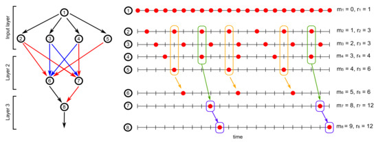
Figure 1. Rhythmic firing in a feedforward neural network.

Given an initial neural firing state $x\left(0\right)=(1,0,0,0,0,0,0,0)$, the dynamical Equation (1) ensures that neurons $1,2,\dots ,5$ in the input layer fire in rhythm $r_1=1,r_2=3,r_3=3,r_4=4,r_5=6$ and in phase $m_1=0,m_2=1,m_3=2,m_4=3,m_5=4$, respectively. In addition, since

$$\begin{array}{c}{x}_6(t+1)=\mathrm{𝟙}\left(5x_2\left(t\right)+3x_3\left(t\right)-x_4\left(t\right)+x_5\left(t\right)-5\right),\end{array}$$

(82)

$$\begin{array}{c}{x}_7(t+1)=\mathrm{𝟙}\left(x_2\left(t\right)-2x_3\left(t\right)+2x_4\left(t\right)-2.5\right),\end{array}$$

(83)

neurons $6,7$ in layer 2 fire in rhythm $r_6=6,r_7=12$ and in phase $m_6=5,m_7=8$, respectively. This is feasible when the summation of incoming signals from neurons $2,5$ to 6 (respectively, from neurons $2,4$ to 7) is largest, and then the firing threshold of neuron 6 (respectively, neuron 7) can be adjusted to sieve out such a rhythmic firing pattern. Similar results can be found on neuron 8 in layer 3, which fires in rhythm $r_8=12$ and in phase $m_8=9$ according to

$$x_8(t+1)=\mathrm{𝟙}\left(-x_6\left(t\right)+3x_7\left(t\right)-2.5\right).$$

(84)

Denote by $\mathrm{\Omega }$ the resulting flow of rhythmic neural firing states from time $\tau$ to $\tau +11$. According to the formula of the pruning map proved in Theorem 2, we see that

$$\begin{array}{c}gcd(r_6,r_2)=3\mathrm{a}\mathrm{n}\mathrm{d}{[m_2+1]}_{gcd(r_6,r_2)}={\left[m_6\right]}_{gcd(r_6,r_2)}=2,\end{array}$$

(85)

$$\begin{array}{c}gcd(r_6,r_3)=3\mathrm{a}\mathrm{n}\mathrm{d}{\left[m_3\right]}_{gcd(r_6,r_3)}={\left[m_6\right]}_{gcd(r_6,r_3)}=2,\end{array}$$

(86)

$$\begin{array}{c}gcd(r_6,r_4)=2\mathrm{a}\mathrm{n}\mathrm{d}{\left[m_4\right]}_{gcd(r_6,r_4)}={\left[m_6\right]}_{gcd(r_6,r_4)}=1,\end{array}$$

(87)

$$\begin{array}{c}gcd(r_6,r_5)=6\mathrm{a}\mathrm{n}\mathrm{d}{[m_5+1]}_{gcd(r_6,r_5)}={\left[m_6\right]}_{gcd(r_6,r_5)}=5,\end{array}$$

(88)

$$\begin{array}{c}gcd(r_7,r_2)=3\mathrm{a}\mathrm{n}\mathrm{d}{[m_2+1]}_{gcd(r_7,r_2)}={\left[m_7\right]}_{gcd(r_7,r_2)}=2,\end{array}$$

(89)

$$\begin{array}{c}gcd(r_7,r_3)=3\mathrm{a}\mathrm{n}\mathrm{d}{\left[m_3\right]}_{gcd(r_7,r_3)}={\left[m_7\right]}_{gcd(r_7,r_3)}=2,\end{array}$$

(90)

$$\begin{array}{c}gcd(r_7,r_4)=4\mathrm{a}\mathrm{n}\mathrm{d}{[m_4+1]}_{gcd(r_7,r_4)}={\left[m_7\right]}_{gcd(r_7,r_4)}=0,\end{array}$$

(91)

$$\begin{array}{c}gcd(r_8,r_7)=12\mathrm{a}\mathrm{n}\mathrm{d}{[m_7+1]}_{gcd(r_8,r_7)}={\left[m_8\right]}_{gcd(r_8,r_7)}=9,\end{array}$$

(92)

and hence

$$\begin{array}{c}{c}_{62}\left(\mathrm{\Omega }\right)<0,c_{63}\left(\mathrm{\Omega }\right)>0,c_{64}\left(\mathrm{\Omega }\right)>0,c_{65}\left(\mathrm{\Omega }\right)<0,\end{array}$$

(93)

$$\begin{array}{c}{c}_{72}\left(\mathrm{\Omega }\right)<0,c_{73}\left(\mathrm{\Omega }\right)>0,c_{74}\left(\mathrm{\Omega }\right)<0,c_{87}\left(\mathrm{\Omega }\right)<0.\end{array}$$

(94)

Then, by neural path pruning described in Equations (7) and (8), the coupling operator can be given by

$$d_{62}>0,d_{63}<0,d_{64}<0,d_{65}>0\mathrm{a}\mathrm{n}\mathrm{d}{d}_{72}>0,d_{73}<0,d_{74}>0,d_{87}>0$$

(95)

which maintain the rhythmic firing pattern of neuron 6 (respectively, neuron 7 and neuron 8) by keeping the largest summation of incoming signals from neurons $2,5$ to 6 (respectively, from neurons $2,4$ to 7 and from neuron 7 to 8). As illustrated by the orange, green, and purple boxes in Figure 1, the coupling operator in Equation (95) fits well with the neurobiological concept of Hebbian synaptic plasticity, meaning that when neurons $2,5$ (respectively, neurons $2,4$ and neuron 7) repeatedly or persistently take part in firing neuron 6 (respectively, neuron 7 and neuron 8), the coupling weights between them are strengthened. Such activity-dependent plasticity between layers of neurons is prone to keep neurons firing in rhythm in the posterior layer.

An experimental setting is defined as follows, showing the performance of rhythm formation in feedforward neural networks. The input rhythm and the layer architecture of feedforward neural networks are specified as in Figure 1. Initially, the coupling weights from prior layers to posterior layers and the firing thresholds of neurons are selected randomly from the interval $[-0.5,0.5]$. When a neuron in layer 2 or 3 fires dynamically, its firing threshold will be adjusted by a positive value 1, otherwise a negative value $-0.1$. In addition, the coupling weights are adjusted according to the coupling operators (with intensity 1 or $-1$) derived from neural path pruning. The transition function of a neuron i is selected to be the Heaviside function defined by Equation (2) or the sigmoid function $\mathcal{S}$ defined by

$$x_i(t+1)=\mathcal{S}\left(\sum _{j=1}^n{a}_{ij}{x}_j\left(t\right)-b_i\right)=\frac{1}{1+e^{-\alpha ({\sum }_{j=1}^n{a}_{ij}{x}_j\left(t\right)-b_i)}},t=0,1,\dots ,$$

(96)

where $\alpha$ is a positive real number. For each round of simulation, we say that rhythm formation occurs in the feedforward neural network if the neuron in layer 3 can persistently fire in rhythm for certain time steps. Specifically, a criterion is defined by k times of neural firing (with the firing state $x_8\left(t\right)>0.8$) in rhythm r with $k·r>500$ during time steps $t=1001$ to 2000. Figure 2 shows the successful rates for rhythm formation in feedforward neural networks, with neurons activating via the Heaviside functions (red line, $100,000$ rounds of simulation) or the sigmoid functions with a selected $\alpha =0.01,0.02,\dots ,0.99,1,2,\dots ,500$ (blue line, 1000 rounds of simulation per $\alpha$). It reveals that rhythm formation can robustly occur in feedforward neural networks, even under the change of the transition functions from the Heaviside functions to the sigmoid functions.

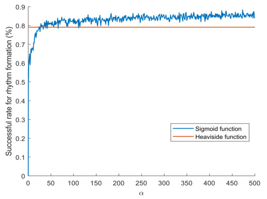
Figure 2. Successful rates for generating rhythmic firing in feedforward neural networks.

4. Conclusions

For neurons firing in rhythm, the pruning map can be formulated in terms of quantities related to rhythmic neural firing. This formulation has the potential to feed crucial control of coupling weights to support the consolidation of rhythms in feedforward neural networks. It reveals a learning rule of feedforward neural networks, which fits well with Hebbian synaptic plasticity for rhythmic pattern formation. Such neural network models can be implemented in relating different kinds of rhythms from input signals to output signals, and hence may be applied to the issues concerning the robot control or pattern recognition with rhythm. We hope that the analysis of pruning maps will stimulate further studies of underlying principles of neural networks concerning how the rhythms interact with each other and organize themselves, providing a theoretical framework mimicking the roles of rhythms in the information processing systems of living organisms.

References

- Strogatz, S.H.; Stewart, I. Coupled oscillators and biological synchronization. Sci. Am. 1993, 269, 68–75. [Google Scholar] [CrossRef] [PubMed]
- Glass, L. Synchronization and rhythmic processes in physiology. Nature 2001, 410, 277–284. [Google Scholar] [CrossRef] [PubMed]
- Smith, H.M. Synchronous flashing of fireflies. Science 1935, 82, 151–152. [Google Scholar] [CrossRef] [PubMed]
- Peskin, C.S. Mathematical Aspects of Heart Physiology; Courant Institute of Mathematical Sciences, New York University: New York, NY, USA, 1975. [Google Scholar]
- Mirollo, R.E.; Strogatz, S.H. Synchronization of pulse-coupled biological oscillators. SIAM J. Appl. Math. 1990, 50, 1645–1662. [Google Scholar] [CrossRef]
- Golubitsky, M.; Stewart, I.; Török, A. Patterns of synchrony in coupled cell networks with multiple arrows. SIAM J. Appl. Dyn. Syst. 2005, 4, 78–100. [Google Scholar] [CrossRef]
- Diesmann, M.; Gewaltig, M.-O.; Aertsen, A. Stable propagation of synchronous spiking in cortical neural networks. Nature 1999, 402, 529–533. [Google Scholar] [CrossRef] [PubMed]
- Grinstein, G.; Linsker, R. Synchronous neural activity in scale-free network models versus random network models. Proc. Natl. Acad. Sci. USA 2005, 102, 9948–9953. [Google Scholar] [CrossRef] [PubMed]
- Schechter, B. How the brain gets rhythm. Science 1996, 274, 339. [Google Scholar] [CrossRef] [PubMed]
- Soto-Treviño, C.; Thoroughman, K.A.; Marder, E.; Abbott, L.F. Activity-dependent modification of inhibitory synapses in models of rhythmic neural networks. Nat. Neurosci. 2001, 4, 297–303. [Google Scholar] [CrossRef] [PubMed]
- Buzsáki, G. Rhythms of the Brain; Oxford University Press: New York, NY, USA, 2006; ISBN 0-19-530106-4. [Google Scholar]
- Hebb, D.O. The Organization of Behavior; Wiley: New York, NY, USA, 1949; ISBN 978-0805843002. [Google Scholar]
- Adams, P. Hebb and Darwin. J. Theoret. Biol. 1998, 195, 419–438. [Google Scholar] [CrossRef] [PubMed]
- Sejnowski, T.J. The book of Hebb. Neuron 1999, 24, 773–776. [Google Scholar] [CrossRef]
- Sumbre, G.; Muto, A.; Baier, H.; Poo, M. Entrained rhythmic activities of neuronal ensembles as perceptual memory of time interval. Nature 2008, 456, 102–106. [Google Scholar] [CrossRef] [PubMed]
- LeCun, Y.; Boser, B.; Denker, J.S.; Henderson, D.; Howard, R.E.; Hubbard, W.; Jackel, L.D. Backpropagation applied to handwritten zip code recognition. Neural Comput. 1989, 1, 541–551. [Google Scholar] [CrossRef]
- He, K.; Zhang, X.; Ren, S.; Sun, J. Deep residual learning for image recognition. In Proceedings of the 2016 IEEE Conference on Computer Vision and Pattern Recognition (CVPR), Las Vegas, NV, USA, 26 June–1 July 2016; pp. 770–778. [Google Scholar]
- Huang, G.; Liu, Z.; van der Maaten, L.; Weinberger, K.Q. Densely connected convolutional networks. In Proceedings of the 2017 IEEE Conference on Computer Vision and Pattern Recognition (CVPR), Honolulu, HI, USA, 21–26 July 2017; pp. 4700–4708. [Google Scholar]
- Girshick, R.; Donahue, J.; Darrell, T.; Malik, J. Rich feature hierarchies for accurate object detection and semantic segmentation. In Proceedings of the 2014 IEEE Conference on Computer Vision and Pattern Recognition (CVPR), Columbus, OH, USA, 23–28 June 2014; pp. 580–587. [Google Scholar]
- Redmon, J.; Divvala, S.; Girshick, R.; Farhadi, A. You only look once: Unified, real-time object detection. In Proceedings of the 2016 IEEE Conference on Computer Vision and Pattern Recognition (CVPR), Las Vegas, NV, USA, 26 June–1 July 2016; pp. 779–788. [Google Scholar]
- He, K.; Gkioxari, G.; Dollar, P.; Girshick, R. Mask R-CNN. In Proceedings of the 2017 IEEE International Conference on Computer Vision (ICCV), Venice, Italy, 22–29 October 2017; pp. 2961–2969. [Google Scholar]
- Zhang, W.; Li, R.; Deng, H.; Wang, L.; Lin, W.; Ji, S.; Shen, D. Deep convolutional neural networks for multi-modality isointense infant brain image segmentation. Neuroimage 2015, 108, 214–224. [Google Scholar] [CrossRef] [PubMed]
- Moeskops, P.; Viergever, M.A.; Mendrik, A.M.; de Vries, L.S.; Benders, M.J.; Išgum, I. Automatic segmentation of MR brain images with a convolutional neural network. IEEE Trans. Med. Imaging 2016, 35, 1252–1261. [Google Scholar] [CrossRef] [PubMed]
- Dolz, J.; Desrosiers, C.; Ayed, I.B. 3D fully convolutional networks for subcortical segmentation in MRI: A large-scale study. Neuroimage 2018, 170, 456–470. [Google Scholar] [CrossRef] [PubMed]
- Shih, M.-H.; Tsai, F.-S. Growth dynamics of cell assemblies. SIAM J. Appl. Math. 2009, 69, 1110–1161. [Google Scholar] [CrossRef]
- Shih, M.-H.; Tsai, F.-S. Decirculation process in neural network dynamics. IEEE Trans. Neural Netw. Learn. Syst. 2012, 23, 1677–1689. [Google Scholar] [CrossRef] [PubMed]
- Shih, M.-H.; Tsai, F.-S. Operator control of interneural computing machines. IEEE Trans. Neural Netw. Learn. Syst. 2013, 24, 1986–1998. [Google Scholar] [CrossRef] [PubMed]
- Tsai, F.-S.; Hsu, S.-Y.; Shih, M.-H. Adaptive tracking control for robots with an interneural computing scheme. IEEE Trans. Neural Netw. Learn. Syst. 2018, 29, 832–844. [Google Scholar] [CrossRef] [PubMed]
© 2019 by the authors. Licensee MDPI, Basel, Switzerland. This article is an open access article distributed under the terms and conditions of the Creative Commons Attribution (CC BY) license (http://creativecommons.org/licenses/by/4.0/).