Cost-Based Optimum Design of Reinforced Concrete Retaining Walls Considering Different Methods of Bearing Capacity Computation

Abstract

This paper investigates the effect of computing the bearing capacity through different methods on the optimum construction cost of reinforced concrete retaining walls (RCRWs). Three well-known methods of Meyerhof, Hansen, and Vesic are used for the computation of the bearing capacity. In order to model and design the RCRWs, a code is developed in MATLAB. To reach a design with minimum construction cost, the design procedure is structured in the framework of an optimization problem in which the initial construction cost of the RCRW is the objective function to be minimized. The design criteria (both geotechnical and structural limitations) are considered constraints of the optimization problem. The geometrical dimensions of the wall and the amount of steel reinforcement are used as the design variables. To find the optimum solution, the particle swarm optimization (PSO) algorithm is employed. Three numerical examples with different wall heights are used to capture the effect of using different methods of bearing capacity on the optimal construction cost of the RCRWs. The results demonstrate that, in most cases, the final design based on the Meyerhof method corresponds to a lower construction cost. The research findings also reveal that the difference among the optimum costs of the methods is decreased by increasing the wall height.

1. Introduction

Reinforced concrete retaining walls (RCRWs) are referred to as structures that withstand the pressure resulting from the difference in the levels caused by embankments, excavations, and/or natural processes. Such situations frequently occur in the construction of several structures, such as bridges, railways, and highways. Due to the frequent application of RCRWs in civil engineering projects, minimizing the construction cost of such structures is an issue of crucial importance.

The satisfaction of both geotechnical and structural design constraints is a key component in the design of RCRWs. In most cases, primary dimensions are initially estimated based on reasonable assumptions and the experience of the designer. Then, in order to reach a cost-effective design while satisfying the design constraints, the design variables (particularly the wall dimensions) need to be revised by using a trial-and-error process, which makes it rather grueling. On the other hand, there is no guarantee that the final design will be the best possible one. To eliminate this problem, which can hinder the designer from reaching a cost-effective solution, and by considering the advances in computational technologies during the recent decades, it makes sense to express the design in the form of a formal optimization problem.

The design optimization of RCRWs has received significant attention during the last two decades. Some of the pertinent works are briefly investigated herein. As a benchmark work, Saribas and Erbatur [1] used a nonlinear programming method and investigated the sensitivity of the optimum solutions to parameters such as backfill slope, surcharge load, internal friction angle of retained soil, and yield strength of reinforcing steel. The simulated annealing (SA) algorithm has been also applied to minimize the construction cost of RCRWs [2,3]. Camp and Akin [4] developed a procedure to design cantilever RCRWs using Big Bang–Big Crunch optimization. They captured the effects of surcharge load, backfill slope, and internal friction angle of the retained soil on the values of low-cost and low-weight designs with and without a base shear key. Khajehzadeh et al. [5] used the particle swarm optimization with passive congregation (PSOPC), claiming that the proposed algorithm was able to find an optimal solution better than the original PSO and nonlinear programming. In their work, the weight, cost, and CO₂ emissions were chosen as the three objective functions to be minimized. Gandomi et al. [6] optimized RCRWs by using swarm intelligence techniques, such as accelerated particle swarm optimization (APSO), firefly algorithm (FA), and cuckoo search (CS). They concluded that the CS algorithm outperforms the other ones. They also investigated the sensitivity of the algorithms to surcharge load, base soil friction angle, and backfill slope with respect to the geometry and design parameters. Kaveh and his colleagues (e.g., [7,8,9,10]) optimized the RCRWs using nature-inspired optimization algorithms, including charged system search (CSS), ray optimization algorithm (RO), dolphin echolocation optimization (DEO), colliding bodies of optimization (CBO), vibrating particles system (VPS), enhanced colliding bodies of optimization (ECBO), and democratic particle swarm optimization (DPSO). Temur and Bekdas [11] employed the teaching–learning-based optimization (TLBO) algorithm to find the optimum design of cantilever RCRWs. They concluded that the minimum weight of the RCRWs decreases as the internal friction angle of the retained soil increases, and increases with the values of the surcharge load. Ukritchon et al. [12] presented a framework for finding the optimum design of RCRWs, considering the slope stability. Aydogdu [13] introduced a new version of a biogeography-based optimization (BBO) algorithm with levy light distribution (LFBBO) and, by using five examples, it was shown that this algorithm outperforms some other metaheuristic algorithms. In this work, the cost of the RCRWs was used as the criterion to find the optimum design. Nandha Kumar and Suribabu [14] adopted the differential evolution (DE) algorithm to solve the design optimization problem of RCRWs. The results of sensitivity analysis showed that width and thickness of the base slab and toe width increases as the height of stem increases. Gandomi et al. [15] studied the importance of different boundary constraint handling mechanisms on the performance of the interior search algorithm (ISA). Gandomi and Kashani [16] minimized the construction cost and weight of RCRWs analyzed by the pseudo-static method. They employed three evolutionary algorithms, DE, evolutionary strategy (ES), and BBO, and concluded that BBO outperforms the others in finding the optimum design of RCRWs. More recently, Mergos and Mantoglou [17] optimized concrete retaining walls by using the flower pollination algorithm, claiming that this method outperforms PSO and GA.

By taking a look at the studies so far reported, it can be noticed that there has been no work done in assessing the effect of using different available methods of determining the bearing capacity on the optimum design of the RCRWs. The current study investigates this important issue. In order to model and design the RCRWs, a code is developed in MATLAB [18]. To reach a design with minimum construction cost, an optimization problem is defined and the construction cost is considered as the single objective function to be minimized. The design criteria, including both geotechnical and structural limitations, are considered as the optimization constraints. The wall geometrical dimensions and the amount of steel reinforcement are used as the design variables. The particle swarm optimization (PSO) [19] algorithm is used to find the optimum solution.

2. Design of Retaining Walls

The design of RCRWs includes two sets of variables. The first set consists of the geometrical dimensions of the concrete wall, namely variables X₁ to X₈, that are defined as shown in Table 1 and depicted graphically in Figure 1. It can be seen that these variables fully define the geometry of the structure.

Table 1. Description of the geometric variables and their lower and upper bounds.

Geometric Variable	Description	Lower Bound	Upper Bound
X1	Width of the base slab	0.4H	0.8H
X2	Toe width	0.1H	0.6H
X3	Thickness at the bottom of the stem	0.2 m	0.5 m
X4	Thickness at the top of the stem	0.2 m	0.4 m
X5	Thickness of the base	0.2 m	0.3H
X6	Distance from the toe to the front face of the shear key	0.5H	0.8H
X7	Width of shear key	0.2 m	0.4 m
X8	Depth of the shear key	0.2 m	0.9 m

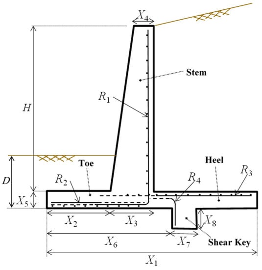
Figure 1. Design variables (X₁ to X₈ and R₁ to R₄), (redesigned based on [4]).

The second set is the amounts of steel reinforcement for four components of the wall—the stem, heel, toe, and shear key. As such, four variables, R₁ to R₄, are introduced to represent the steel reinforcement of the different components, as shown in Table 2. In this paper, a total of 223 possible reinforcement configurations were used, resulting from the combinations of using 3–28 evenly spaced bars, with varying sizes (bar diameter) from 10 to 30 mm. It is worth mentioning that the combinations used for the steel reinforcement, as listed in Table 3, are obtained such that the allowable minimum and maximum amount of steel area per unit meter length of the wall are satisfied as per ACI318-14 code [20].

Table 2. Description of the reinforcement variables.

Reinforcement Variable	Description
R1	Vertical steel reinforcement of the stem
R2	Horizontal steel reinforcement of the toe
R3	Horizontal steel reinforcement of the heel
R4	Vertical steel reinforcement of shear key

Table 3. Steel reinforcement combinations (adopted from [4]).

Index Number	Bars Quantity and Size (R)	Bars Cross-Sectional Area (cm2) (in Ascending Order)
1	3ϕ10	2.356 (lower bound)
2	4ϕ10	3.141
3	3ϕ12	3.392
4	5ϕ10	3.926
5	4ϕ12	4.523
.	.	.
.	.	.
221	16ϕ30	113.097
222	17ϕ30	120.165
223	18ϕ30	127.234 (upper bound)

The allowable value of spacing between longitudinal bars (ds_all) is defined as follows [20]:

$$d{s}_{\mathrm{all}}=\max \{25mm,d_{\mathrm{bl}},1.33d_{\max }\},$$

(1)

in which d_bl and d_max are the diameter of longitudinal reinforcements and diameter of greatest aggregate of concrete, respectively. For the purposes of steel reinforcement design, ACI318-14 code [20] has been considered.

In the design of RCRWs, geotechnical stability control and the satisfaction of the structural requirements are mandatory. In geotechnical design, the stability of the structure shall be controlled against possible overturning, sliding, and bearing capacity failure modes. On the other hand, in the structural design phase, each component of the structure, including the stem, toe, heel, and shear key, shall be checked against shear and moment demands [21]. Figure 2 shows all the forces acting on the retaining wall. As shown in this figure, P_a is the resultant force of the active pressure p_a per unit length of the wall; Q_s is the resultant force of the distributed surcharge load q; W_C is the weight of all sections of the reinforced concrete wall; W_S and W_T are defined as the weight of backfill behind the retaining wall and the weight of the soil on the toe, respectively; P_p is the resultant force due to the passive pressure (p_p) on the front face of the toe and shear key per unit length of the wall; P_b is the resultant force caused by the pressure acting on the base soil; q_max and q_min are the maximum and minimum soil pressure intensity at the toe and the heel of the retaining wall, respectively. In this paper, the water level and the seismic actions were not considered in computing the forces acting on the RCRWs. The pressure distributions on the base and retaining soil have also been illustrated in Figure 2.

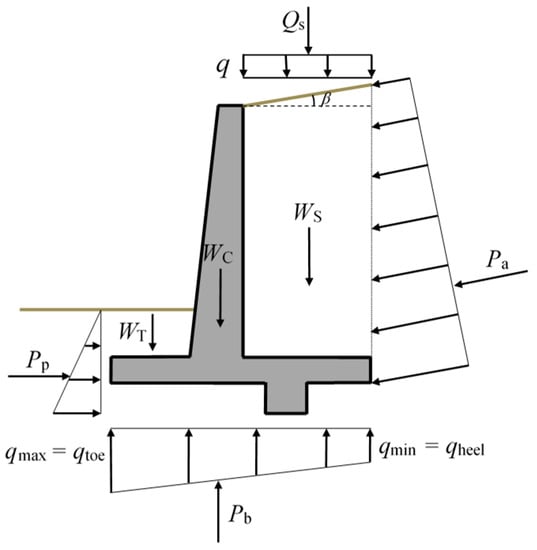
Figure 2. Forces acting on the retaining wall (redesigned based on [6]).

In this study, Rankine theory was used to evaluate the active and passive forces acting on the unit length of the retaining wall (p_a and p_p, respectively), and they are computed as follows [21]:

$$p_{\mathrm{a}}=\frac{1}{2}{k}_{\mathrm{a}}{\gamma }_{\mathrm{rs}}{H^{\prime }}^2+k_{a}q{H}^{\prime },$$

(2)

$$p_{\mathrm{p}}=\frac{1}{2}{k}_{\mathrm{p}}{\gamma }_{\mathrm{bs}}{D^{\prime }}^2+2c_{\mathrm{bs}}\sqrt{k_{\mathrm{p}}}{D^{\prime }}^2,$$

(3)

where k_a and k_p are the Rankine active and passive earth pressure coefficients, respectively; D′ is the buried depth of shear key; γ_rs is the unit weight of backfill; H′ is the height of the soil located on the embedment depth of the base slab at the edge of the heel; γ_bs and ff_bs are the unit weight and the cohesion of soil in front of the toe and beneath the base slab, respectively. k_a is computed as [21]:

$$k_{\mathrm{a}}=\cos \beta \frac{\cos \beta -\sqrt{{\cos }^2\beta -{\cos }^2{\varphi }_{\mathrm{rs}}}}{\cos \beta +\sqrt{{\cos }^2\beta -{\cos }^2{\varphi }_{\mathrm{rs}}}},$$

(4)

in which β and ϕ_rs are the slope and internal friction angle of the back fill, respectively; k_p is computed as follows [21]:

$$k_{\mathrm{p}}={\tan }^2(45+\frac{{\varphi }_{\mathrm{bs}}}{2}),$$

(5)

in which ϕ_bs (in degrees) is the internal friction angle of soil in front of the toe and beneath the base slab.

2.1. Geotechnical Stability Demands

A retaining wall may fail due to overturning about the toe, sliding along the base slab, and the loss of bearing capacity of the soil supporting the base [21]. The checks for these three failure modes are described in this section. The safety factor against overturning about the toe is defined as follows:

$$F{S}_{\mathrm{O}}=\frac{{\displaystyle \sum M_{\mathrm{R}}}}{{\displaystyle \sum M_{\mathrm{O}}}},$$

(6)

in which ∑M_R is the sum of the moments tending to resist against overturning about the toe and ∑M_O is the sum of the moments tending to overturn the wall about the toe [21]. The safety factor against sliding along the base slab is computed as follows:

$$F{S}_{\mathrm{S}}=\frac{{\displaystyle \sum F_{\mathrm{R}}}}{{\displaystyle \sum F_{\mathrm{D}}}},$$

(7)

where ∑F_R is the sum of the resisting forces against the sliding and ∑F_D is the sum of the horizontal driving forces.

The safety factor against bearing capacity failure mode is computed by:

$$F{S}_{\mathrm{B}}=\frac{q_{\mathrm{u}}}{q_{\max }},$$

(8)

in which q_u is the ultimate bearing capacity of the soil supporting the base slab. The ultimate bearing capacity is the load per unit area of the foundation at which shear failure occurs in the soil. For retaining walls, q_u is computed as follows [21]:

$$q_{\mathrm{u}}=c_{\mathrm{bs}}{N}_{\mathrm{c}}{F}_{\mathrm{cs}}{F}_{\mathrm{cd}}{F}_{\mathrm{ci}}+q{N}_{\mathrm{q}}{F}_{\mathrm{qs}}{F}_{\mathrm{qd}}{F}_{\mathrm{qi}}+0.5{\gamma }_{\mathrm{bs}}{B}^{\prime }{N}_{\mathsf{\gamma }}{F}_{\mathsf{\gamma }\mathrm{s}}{F}_{\mathsf{\gamma }\mathrm{d}}{F}_{\mathsf{\gamma }\mathrm{i}},$$

(9)

where:

$$q={\gamma }_{\mathrm{bs}}D,$$

(10)

in which D is the embedment depth of the toe (base slab). B′ is computed as:

$$B^{\prime }=B-2e,$$

(11)

where B is the width of the base slab. As mentioned earlier, q_max and q_min, which are the maximum and minimum stresses occurring at the end of the toe and heel of the structure, respectively, are computed as follows [21]:

$$q_{\min }^{\max }=\frac{{\displaystyle \sum V}}{B}\left(1\pm \frac{6e}{B}\right),$$

(12)

where e is defined as the eccentricity of the resultant force, which can be computed as follows:

$$e=\frac{B}{2}-\frac{{\displaystyle \sum M_{\mathrm{R}}}-{\displaystyle \sum M_{\mathrm{O}}}}{{\displaystyle \sum V}}.$$

(13)

Note that if e becomes greater than B/6, then some tensile stress will be applied at the soil located under the heel section. In such a case, since the tensile strength of soil is negligible, design and calculations should be repeated.

In Equation (9), the N coefficients are used for the modification of the bearing capacity value and the F coefficients are used for the modification of the shape, depth, and inclination factors. The bearing capacity factors N_c, N_q, and N_γ are, respectively, the contributions of cohesion, surcharge, and unit weight of soil to the ultimate load-bearing capacity [21]. Some of these coefficients vary in accordance with the method used, resulting in different values for q_u. Hence, this issue could affect the final design of the RCRWs. In this paper, the effects of three methods of Meyerhof [22], Hansen [23], and Vesic [24] in computing q_u were investigated, particularly their effect on the optimized construction cost of the RCRWs. The N and F coefficients corresponding to each of the three design methods are listed in Appendix A.

2.2. Structural Requirements

The moment and shear capacity of all components of the retaining wall must be greater than their corresponding demands. The flexural strength of each component can be computed as follows [20]:

$$M_{\mathrm{n}}={\varphi }_{\mathrm{m}}{A}_{\mathrm{s}}{f}_{\mathrm{y}}\left(d-\frac{a}{2}\right),$$

(14)

in which ϕ_m is known as the nominal strength coefficient (equal to 0.9 [20]); A_s is the cross-sectional area of the steel reinforcement; f_y is the yield strength of steel; d is the effective depth of the cross section; and a is the depth of the compressive stress block. The shear strength is estimated by [20]:

$$V_{\mathrm{n}}=0.17{\varphi }_{\mathrm{v}}\sqrt{f_{\mathrm{c}}}bd,$$

(15)

where ϕ_v is the nominal strength coefficient (equal to 0.75 [20]); f_c is the specified compressive strength of concrete; and b is the width of the cross section.

2.2.1. Flexural Moment and Shear Force Demands of Stem

As shown in Figure 2, by considering the active force acting on the unit length of the wall due to surcharge load and the weight of the backfill on the stem, the critical section for flexural moment is at the intersection of the stem with the base slab. In addition, the critical section for shear force is at a distance d_s from the intersection of the stem with the foot slab, defined as d_s = X₃ − C_C, where C_C is the concrete cover. The flexural moment and shear force demands of the stem at its critical section are computed by the following equations:

$$M_{\mathrm{s}}=1.6[\frac{1}{2}(\left(k_{\mathrm{a}}q{H}^2\right)+\left(\frac{1}{3}{k}_{\mathrm{a}}{\gamma }_{\mathrm{rs}}{H}^3\right))]\cos \beta ,$$

(16)

$$V_{\mathrm{s}}=1.6\left((k_{\mathrm{a}}q\left(H-d_{\mathrm{s}}\right)+\frac{1}{2}{k}_{\mathrm{a}}{\gamma }_{\mathrm{rs}}{\left(H-d_{\mathrm{s}}\right)}^2\right)\cos \beta .$$

(17)

2.2.2. Flexural Moment and Shear Force Demands of Toe Slab

The effective forces on the toe slab include the soil weight on the toe slab, the weight of the toe concrete slab, and the force caused by earth pressure under the toe slab. The foot of the front face of the stem is the critical section for flexural moment and the critical section for shear force is formed at a distance d_t from the front face of the stem (d_t = X₅ − C_C). The flexural moment and shear force demands of the toe slab at its critical section are computed by the following equations [6]:

$$M_{\mathrm{t}}=[1.6(\frac{q_2}{6}+\frac{q_{\max }}{3})-0.9({\gamma }_{\mathrm{c}}{X}_5+{\gamma }_{\mathrm{bs}}(D-X_5))]l_{\mathrm{toe}}^2,$$

(18)

$$V_{\mathrm{t}}=[1.6\left(\frac{q_{dt}+q_{\max }}{2}\right)-0.9({\gamma }_{\mathrm{c}}{X}_5+{\gamma }_{\mathrm{bs}}(D-X_5))].\left(l_{\mathrm{toe}}-dt\right),$$

(19)

where q₂ is the soil pressure intensity at the foot of the front face of the stem; γ_c is the unit weight of concrete; l_toe is the length of the toe slab; and q_dt is the soil pressure at a distance d_t from the foot of the stem front face.

2.2.3. Flexural Moment and Shear Force Demands of Heel Slab

The forces acting on the heel section include the soil weight of top of the heel slab, the weight of the heel concrete slab, the surcharge load, and the force resulting from earth pressure under the heel slab. The foot of the stem back face is the critical section for flexural moment and the critical section for shear force is at a distance d_h from the foot of the stem back face (d_h = X₅ − C_C). The flexural moment and shear force demands of the heel slab at its critical section are computed by the following equations [6]:

$$M_{\mathrm{h}}=[\left(\frac{1.6q+1.2{\gamma }_{\mathrm{c}}{X}_5+1.2{\gamma }_{\mathrm{rs}}H}{2}\right)+\frac{1.2W_{\mathrm{bs}}}{3}-\left(\frac{q_1+2q_{\min }}{6}\right)]l_{\mathrm{heel}}^2,$$

(20)

$$V_{\mathrm{h}}=[1.6q+1.2{\gamma }_{\mathrm{c}}{X}_5+1.2{\gamma }_{\mathrm{rs}}H+1.2\frac{W_{\mathrm{bs}}+W_{\mathrm{bsdh}}}{2}-0.9\frac{q_{\mathrm{dh}}+q_{\min }}{2}]\left(l_{\mathrm{heel}}-d_{\mathrm{h}}\right),$$

(21)

in which W_bs is the maximum load due to triangular backfill soil weight at the top of the heel slab; q₁ is the soil pressure intensity at the foot of the stem back face; l_heel is the length of retaining wall heel; W_bsdh is the load resulting from triangular backfill soil weight; and q_dh is the intensity of soil pressure at a distance d_h from the stem back face.

3. Optimization Problem

3.1. Formulation

Optimization problems can be divided into two large groups in general—constrained and unconstrained problems. Because of the limitations required for the design of structures, the optimum design of RCRWs is a constrained optimization problem, which can be expressed as follows [25]:

$$\begin{array}{l}MinimizeF(\mathit{x})subjectedto{g}_{\mathrm{i}}(\mathit{x})\le 0\\ (\mathrm{i}=1,2,\dots ,m;x_{\mathrm{j}}\in R^{\mathrm{d}},\mathrm{j}=1,2,\dots ,n)\end{array}$$

(22)

in which F(x) is the objective function; g_i(x) is the i-th constraint; m and n are the total number of constraints and design variables, respectively; R^d is a given set of discrete values from which the individual design variables x_j can take values. In this paper, an exterior penalty function method was used to transform the constrained structural optimization problem into an unconstrained one, as follows [26]:

$$\Phi (\mathit{x},r_{\mathrm{p}})=F(\mathit{x})\left[1+r_{\mathrm{p}}{\displaystyle \sum _{\mathrm{r}=1}^{\mathrm{m}}\left(\max (\frac{g_{\mathrm{r}}}{g_{\mathrm{r},\mathrm{all}}}-1,0)\right)}\right],$$

(23)

where ϕ is the pseudo (penalized) objective function; g_r and g_r,all are the r-th constraint and its allowable value, respectively; and r_p is a positive penalty parameter, which in this study was assumed to be equal to 25.

3.2. Objective Function

In this work, the initial construction cost CC_RCRW of the RCRW was considered the single objective function of the optimization problem, to be minimized. The objective function was defined as follows:

$$C{C}_{\mathrm{RCRW}}=C_{\mathrm{c}}{V}_{\mathrm{c}}+C_{\mathrm{st}}{W}_{\mathrm{st}},$$

(24)

where C_c and C_st are the cost per unit volume of concrete and the cost per unit weight of steel reinforcement, respectively; V_c and W_st are the volume of concrete and weight of steel per unit length of the retaining wall, respectively. It is worth noting that the cost of the formwork, casting concrete, vibration, and generally all related labor costs were taken into consideration in the parameter C_c. In addition, the earthwork cost was not considered in the calculation of the total cost of the RCRWs.

3.3. Design Constraints

Two sets of constraints are considered for the optimum design of a RCRW. The first set (four constraints) is related to geotechnical requirements (wall stability). Of these, the first three are considered to provide safety factors against overturning, sliding, and bearing capacity failure modes, as shown below [21]:

$$g_1=\frac{F{S}_{\mathrm{O}}}{F{S}_{\mathrm{O},\mathrm{all}}}-1\ge 0,$$

(25)

$$g_2=\frac{F{S}_{\mathrm{S}}}{F{S}_{\mathrm{S},\mathrm{all}}}-1\ge 0,$$

(26)

$$g_3=\frac{F{S}_{\mathrm{B}}}{F{S}_{\mathrm{B},\mathrm{all}}}-1\ge 0,$$

(27)

in which FS_O, FS_S, and FS_B are the safety factor demands against overturning, sliding, and bearing capacity failure modes, respectively, and FS_O,all, FS_S,all, and FS_B,all are their allowable values.

The fourth constraint of the first set is used to avoid the presence of tensile stresses on the base soil, as follows:

$$g_4=q_{\min }\ge 0.$$

(28)

The second set of constraints is related to the structural requirements having to do with providing the required strength of wall components and reinforcement arrangements in their cross sections, in accordance with ACI318-14 [20]. To design the structural sections, the reinforcement area at each section of the retaining wall should satisfy the allowable amounts of the reinforcement area, as follows:

$$g_{\text{5–8}}={\left(\frac{A_{\mathrm{s}}}{A_{\mathrm{s},\min }}\right)}_{\mathrm{st}}-1\ge 0,$$

(29)

$$g_{\text{9–12}}={\left(\frac{A_{\mathrm{s},\max }}{A_{\mathrm{s}}}\right)}_{\mathrm{st}}-1\ge 0,$$

(30)

in which A_s,min and A_s,max are the minimum and maximum allowable area of steel reinforcement in accordance with the code, and A_s is defined as the cross-sectional area of steel reinforcement in each section. The subscript st refers to all sections of the RCRW including stem, heel, toe and shear key, and similarly subscripts 5 to 8 are used for the stem, toe, heel and shear key, respectively. The same is also the case for subscripts 9 to 12.

As mentioned earlier, the moment and shear capacities of all sections of the retaining wall should be greater than the corresponding demands, namely:

$$g_{\text{13–16}}={\left(\frac{M_{\mathrm{n}}}{M_{\mathrm{d}}}\right)}_{\mathrm{st}}-1\ge 0$$

(31)

$$g_{\text{17–20}}={\left(\frac{V_{\mathrm{n}}}{V_{\mathrm{d}}}\right)}_{\mathrm{st}}-1\ge 0$$

(32)

In the equations above, M_n and V_n are the moment and shear nominal capacity, and M_d and V_d are the moment and shear demands, respectively. M_n and V_n are the flexural moment and shear strength formulated before. The subscripts 13 to 16 are for stem, toe, heel, and shear key. The same is true for subscripts 17 to 20.

The following geometric constraints are also applied to avoid an impossible or impracticable shape of the wall:

$$g_{21}=\frac{X_1}{X_2+X_3}-1\ge 0,$$

(33)

$$g_{22}=\frac{X_1}{X_6+X_7}-1\ge 0.$$

(34)

The minimum development length of the steel reinforcement bars should be considered for all the structural components. At first, the minimum basic development length l_db against the allowable space is checked. If the available space is not enough, a hook is added to achieve the additional development length. In this case, a minimum hook development length l_dh and minimum hook length of 12d_bh (d_bh is the diameter of the hooked bar) should be satisfied. The following limitations are considered for stem, toe, heel, and shear key in the design, respectively:

$$g_{23}=\frac{l_{\mathrm{db},\mathrm{stem}}}{X_5-C_{\mathrm{C}}}-1\ge 0or{g}_{23}=\frac{l_{\mathrm{dh},\mathrm{stem}}}{X_5-C_{\mathrm{C}}}-1\ge 0,$$

(35)

$$g_{24}=\frac{l_{\mathrm{db},\mathrm{toe}}}{X_1-X_2-C_{\mathrm{C}}}-1\ge 0or{g}_{24}=\frac{12d_{\mathrm{b},\mathrm{toe}}}{X_5-C_{\mathrm{C}}}-1\ge 0,$$

(36)

$$g_{25}=\frac{l_{\mathrm{db},\mathrm{heel}}}{X_2+X_3-C_{\mathrm{C}}}-1\ge 0or{g}_{25}=\frac{12d_{\mathrm{b},\mathrm{heel}}}{X_5-C_{\mathrm{C}}}-1\ge 0,$$

(37)

$$g_{26}=\frac{l_{\mathrm{db},\mathrm{key}}}{X_5-C_{\mathrm{C}}}-1\ge 0or{g}_{26}=\frac{l_{\mathrm{dh},\mathrm{key}}}{X_5-C_{\mathrm{C}}}-1\ge 0,$$

(38)

It should be noted that the inequalities g₂₃ to g₂₆ as described in Equations (35)–(38) were actually not considered as design constraints in the present study. In fact, during the optimization process, the required development lengths were simply considered and their role in steel cost was computed and added to the construction cost. The cost of shrinkage reinforcement was also added to the total construction cost. Another important point is that the other constraints on the arrangements of steel bars in the wall sections, such as the number of allowable bars, bar size, and bar spacing, were all considered in the optimum design, as can be seen in Table 2.

3.4. PSO Algorithm

The successful application of the particle swarm optimization (PSO) algorithm in the optimum design of RC structures has been reported in the literature (e.g., [26,27,28,29,30,31,32,33]). In this paper, the PSO algorithm was used to optimize RCRWs. The algorithm was originally developed by Kennedy and Eberhart [19] in the mid-1990s, and was first applied to simulate the social behavior of fish schooling and bird flocking as part of a socio-cognitive research. The PSO algorithm is considered a metaheuristic algorithm that optimizes a problem by iteratively trying to improve a candidate solution. It solves a problem by having a population of candidate solutions called particles. Each particle moves through the search space and its position is updated according to (a) its local best known position, and (b) the best known position for the whole swarm in the search space. Finally, the objective function is calculated for each particle and the fitness values of the candidate solutions are assessed to discover which position in the search space is the best. The algorithm searches for the optimum by adjusting the trajectory of each particle of the swarm in the multi-dimensional design space, in terms of paths created by positional vectors in a quasi-random manner. After finding the best values of position and velocity in each iteration k, these vectors are updated using the following equations:

$${\mathit{X}}_{\mathrm{i},\mathrm{k}+1}={\mathit{X}}_{\mathrm{i},\mathrm{k}}+{\mathit{V}}_{\mathrm{i},\mathrm{k}+1},$$

(39)

$${\mathit{V}}_{\mathrm{i},\mathrm{k}+1}=w_{\mathrm{k}}{\mathit{V}}_{\mathrm{i},\mathrm{k}}+c_1{r}_1\left({\mathit{P}}_{\mathrm{i},\mathrm{k}}-{\mathit{X}}_{\mathrm{i},\mathrm{k}}\right)+c_2{r}_2\left({\mathit{P}}_{\mathrm{g},\mathrm{k}}-{\mathit{X}}_{\mathrm{i},\mathrm{k}}\right),$$

(40)

in which for the i-th particle, X_i,k and V_i,k are the current position vector and velocity vector at iteration k, respectively; P_i,k is the best position that the particle has visited; P_g,k is the global best position obtained so far by all the particles in the population; r₁ and r₂ are random numbers drawn from a uniform distribution in the range of [0, 1]; c₁ and c₂ are constants, called cognitive and social scaling parameters, and are usually in the range of [0, 2]; w_k known as the inertia weight, has a pivotal role in updating the position and the velocity vectors. In fact, this parameter is used to stabilize the motion of the particles, making the algorithm converge more quickly. In this paper, a linear weight-updating rule was implemented as follows:

$$w_{\mathrm{k}}=w_{\max }-\frac{w_{\max }-w_{\min }}{k_{\max }}k,$$

(41)

in which w_max and w_min are the upper and lower bounds of the current weight w_k; and k_max is the maximum number of iterations used. Figure 3 shows a schematic view for the PSO algorithm, i.e., how a particle’s position is updated from one iteration to another toward finding the global optimum.

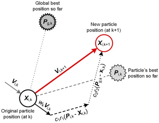
Figure 3. A schematic view for describing particle swarm optimization (PSO).

4. Methodology

As previously mentioned, although many studies have been implemented to optimize the retaining wall design, no studies have been conducted so far investigating the effect of various methods of determining the parameters of the soil ultimate bearing capacity on the design optimization of these structures. The current study deals with this issue and, in particular, the effect of using the methods developed by Meyerhof, Hansen, and Vesic (respectively abbreviated as MM, HM, and VM hereafter) on the cost of the retaining wall. For this purpose, a database containing discrete values of the mentioned variables (X₁ to X₈ and R₁ to R₄) was generated. Then, the PSO algorithm was used to solve the optimum design problem defined above. All the process of optimum design was implemented via a code written in MATLAB [18]. The flowchart of the design optimization process is shown in Figure 4. The next section investigates the effects of the above three methods on the optimum design of RCRWs.

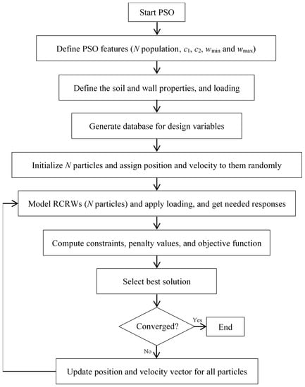
Figure 4. The flowchart of the design optimization of reinforced concrete retaining walls (RCRWs).

5. Design Examples

5.1. Assumptions

Three different RCRWs with different heights of 4.0, 5.5, and 7.0 m were considered for all three methods examined (MM, HM, and VM). A reasonable incremental step of 0.01 m was considered for the geometric variables. As shown in Table 3, a set of discrete values was considered for the steel reinforcement. It should be noted that the cross-sectional area of the steel reinforcement bars per unit length of the wall (1 m) was used during the optimization process, therefore, the number of used bars (n₁ to n₄) needs to be obtained. All the values assumed for the modeling and design of the RCRWs are listed in Table 4.

Table 4. Values of input parameters for Examples 1, 2, and 3.

Parameter	Symbol	Value	Unit
		Examples 1–3
Height of stem	H	4.0, 5.5, and 7.0	m
Steel yield strength	fy	400	MPa
Shrinkage and temperature reinforcement ratio	ρst	0.002	-
Concrete compressive strength	fc	21	MPa
Concrete cover	CC	7	cm
Unit weight of concrete	γc	23.5	kN/m3
Unit weight of steel bars	γs	78.5	kN/m3
Surcharge load	q	15	kPa
Backfill slope	β	5	degrees
Internal friction angle of backfill	φrs	36	degrees
Unit weight of backfill	γrs	17.5	kN/m3
Internal friction angle of base soil	φbs	39	degrees
Cohesion of base soil	cbs	0	kPa
Unit weight of base soil	γbs	20	kN/m3
Embedment depth of the toe	D	0.75	m
Cost of steel per unit of mass	Cst	0.4	$/kg
Cost of concrete per unit of volume	Cc	40	$/m3

Because of the stochastic nature of the PSO algorithm, 20 independent runs were conducted for each case study corresponding to each method (MM, HM, and VM). In the PSO algorithm, the population was 20 and the maximum number of iterations was set to 6000; both c₁ and c₂ parameters were assumed to be equal to 2; w_min and w_max as the minimum and maximum value of the weight w_k, respectively, were considered to be 0.4 and 0.9.

5.2. Results and Discussion

After implementation of the optimization procedure, the best run among the 20 runs was chosen. The convergence history of all examples as Example 1 with H = 4.0 m, Example 2 with H = 5.5 m, and Example 3 with H = 7.0 m are shown in Figure 5, Figure 6 and Figure 7, respectively. The convergence plots, which correspond to the best runs, start with a larger value of the cost, which is then minimized by the PSO algorithm at the final iteration. Note that since the optimization procedure was performed for a unit meter length of the wall, all the presented costs are per meter of length of the wall.

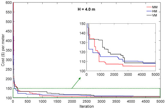
Figure 5. Convergence history of objective function—Example 1.

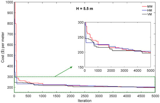
Figure 6. Convergence history of objective function—Example 2.

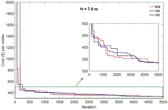
Figure 7. Convergence history of objective function—Example 3.

The optimum design variables, including the geometrical dimensions and the amounts of steel reinforcement for the three examples, are presented in Table 5, Table 6 and Table 7. As can be seen, all the results were within their allowable ranges defined in Table 1 and Table 3. The last two columns of each table present the difference in the design variables for HM and VM with respect to MM as the chosen benchmark method. Based on the results, it can be noted that in general, the dimensions of X₁, X₄, X₆, X₇, and X₈ had relatively low sensitivity to the method used, while the other dimensions, namely X₂ and X₅, were quite sensitive. Concerning X₃, it seems to be sensitive to the method used merely for the case of wall height 4.0 m. The amounts of steel reinforcement (variables R₁, R₂, R₃, and R₄) were highly dependent on the method used.

Table 5. Optimum design variables and comparison of the methods for Example 1—H = 4.0 m.

Variable	Method			Difference (%)
	MM	HM	VM	100 × (HM − MM)/MM	100 × (VM − MM)/MM
X1	2.33	2.47	2.38	6.01	2.15
X2	0.88	1.03	1.05	17.05	19.32
X3	0.37	0.34	0.32	−8.11	−13.51
X4	0.20	0.20	0.20	0.00	0.00
X5	0.24	0.25	0.27	4.17	12.50
X6	2.01	2.01	2.05	0.00	1.99
X7	0.26	0.27	0.28	3.85	7.69
X8	0.23	0.22	0.24	−4.35	4.35
R1	13ϕ12	20ϕ10	21ϕ10	6.84	12.18
R2	13ϕ10	9ϕ12	14ϕ10	−0.31	7.69
R3	13ϕ10	12ϕ10	9ϕ12	0.00	8.00
R4	6ϕ12	14ϕ10	9ϕ10	62.04	4.17

Table 6. Optimum design variables and comparison of the methods for Example 2—H = 5.5 m.

Variable	Method			Difference (%)
	MM	HM	VM	100 × (HM − MM)/MM	100 × (VM − MM)/MM
X1	3.20	3.24	3.16	1.25	−1.25
X2	0.99	1.19	1.33	20.20	34.34
X3	0.47	0.48	0.46	2.13	−2.13
X4	0.21	0.20	0.20	−4.76	−4.76
X5	0.35	0.38	0.36	8.57	2.86
X6	2.78	2.88	2.85	3.60	2.52
X7	0.28	0.26	0.29	−7.14	3.57
X8	0.23	0.20	0.25	−13.04	8.70
R1	13ϕ16	22ϕ12	13ϕ16	−4.81	0.00
R2	5ϕ16	5ϕ20	11ϕ14	56.25	68.44
R3	11ϕ14	16ϕ10	7ϕ14	−25.79	−36.36
R4	12ϕ10	7ϕ16	7ϕ12	49.33	−16.00

Table 7. Optimum design variables and comparison of the methods for Example 3—H = 7.0 m.

Variable	Method			Difference (%)
	MM	HM	VM	100 × (HM − MM)/MM	100 × (VM − MM)/MM
X1	4.04	3.90	3.79	−3.47	−6.19
X2	1.34	1.51	1.76	12.69	31.34
X3	0.49	0.48	0.48	−2.04	−2.04
X4	0.21	0.21	0.20	0.00	−4.76
X5	0.45	0.49	0.56	8.89	24.44
X6	3.75	3.52	3.50	−6.13	−6.67
X7	0.27	0.26	0.27	−3.70	0.00
X8	0.21	0.21	0.21	0.00	0.00
R1	19ϕ18	11ϕ24	19ϕ18	2.92	0.00
R2	14ϕ12	16ϕ12	17ϕ12	14.29	21.43
R3	16ϕ14	23ϕ10	22ϕ10	−26.66	−29.85
R4	5ϕ18	22ϕ10	7ϕ12	35.80	−37.78

To show the convergence of the optimization process to the optimum solution, the best solutions in each iteration corresponding to Example 1 (with H = 4.0 m) considering the MM case are shown together in Figure 8. Based on this figure, PSO found the optimum solution in the design space very well. In addition, the optimum shapes of the three examples with consideration of the three methods of MM, HM, and VM are shown in Figure 9. From this figure, it can be seen that the three methods resulted in different designs (geometrical dimensions) for all the optimum RCRWs with different heights.

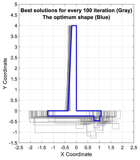
Figure 8. The candidate solutions and the final optimum shape (for H = 4.0 m, corresponding to the MM method).

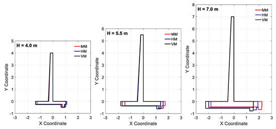
Figure 9. Optimal dimensions of the RCRWs for all examples with the three methods.

Figure 10, Figure 11 and Figure 12 show the demand to capacity ratios of the constraints (all constraints g_1–3 and g_5–20, except for the constraint g₄ on q_min) for the optimum solutions. As can be seen, all the corresponding values were less than 1.0, indicating that the optimum solutions have satisfied all the design constraints.

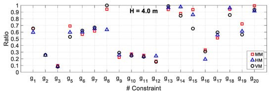
Figure 10. Demand to capacity ratio for Example 1.

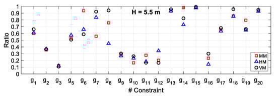
Figure 11. Demand to capacity ratio for Example 2.

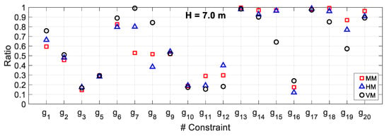
Figure 12. Demand to capacity ratio for Example 3.

The constraint on the soil pressure intensity under the heel (q_min), described as constraint g₄ in Equation (28), which is one of the fundamental constraints in the retaining walls design, has been excluded from the figures, yet it is examined in detail in Table 8. As described earlier, if q_min is negative, it means that some tensile stress is developed at the end of the heel, which is undesirable due to the negligible tensile strength of the soil. The final values for q_min corresponding to each example and method are listed in Table 8. As can be seen, all the values are greater than zero, indicating that no tensile stress appears beneath the heel slab of the RCRWs.

Table 8. q_min (constraint g₄) values for all three examples and all three design methods.

Variable	Example 1—H = 4.0 m			Example 2—H = 5.5 m			Example 3—H = 7.0 m
	MM	HM	VM	MM	HM	VM	MM	HM	VM
qmin	16.15	26.37	17.74	29.60	31.75	23.70	40.61	27.28	9.22

Next, the construction cost of the optimum designs was examined. The concrete, steel, and total cost for all of the optimum RCRWs with different heights, considering the three methods, are listed in Table 9. As can be seen, for H = 4.0 m and H = 7.0 m, the MM resulted in the minimum cost compared with the other two methods; also, the cost for HM was less than that for VM. For H = 5.5 m, the VM had the minimum cost and the cost for MM was less than that for HM. In addition, based on the results of Table 9 and as also shown in Table 5, Table 6 and Table 7, the provided amounts of reinforcement varied depending on the method used. Moreover, it was shown that the differences among the methods decreased with increasing the height of the RCRWs.

Table 9. Cost of optimum RCRWs for different heights considering the three methods.

Variable	Example 1—H = 4.0 m			Example 2—H = 5.5 m			Example 3—H = 7.0 m
	MM	HM	VM	MM	HM	VM	MM	HM	VM
Concrete ($)	70.07	70.60	70.27	122.00	126.39	120.80	172.15	175.37	184.04
Steel ($)	34.96	37.34	38.19	77.07	76.64	75.89	160.45	160.19	152.04
Total ($)	105.04	107.94	108.46	199.08	203.03	196.68	332.61	335.56	336.08
Diff. (%) to MM for total cost	-	2.76	3.26	-	1.99	−1.20	-	0.89	1.04

Figure 13 reveals the variation in cost components (concrete and steel materials) to total cost ratio with respect to the RCRW heights for each method. Based on this figure, it can be concluded that the concrete cost was reduced from 65.64% 52.93% on average with increasing the height, and the steel cost was increased from 34.36% to 47.07% on average with increasing the height.

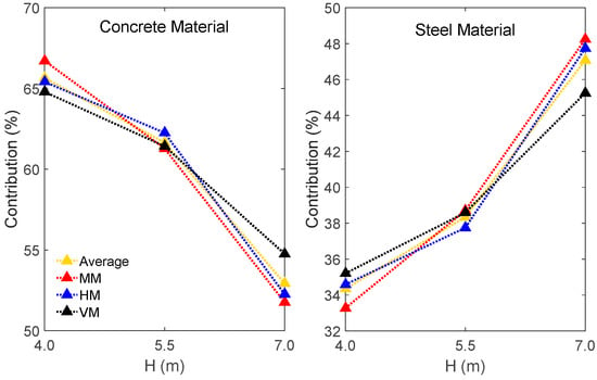
Figure 13. The contribution of concrete and steel materials in total cost for optimum RCRWs.

5.3. Comparative Study

In order to make a comparison with the literature, a specific example was chosen from the work conducted by Gandomi et al. [6] (Example 2, case 1 of the work [6] for β = 0°, see corresponding Table 12 of that work). Using the methodology of the present work, all three methods of MM, HM, and VM were considered for the comparison. The results are listed in Table 10. As can be seen in this table, the results obtained for MM, HM, and VM were slightly different to those by Gandomi et al. [6], at least as far as the optimum cost is concerned. This can be attributed to the different analysis method and the different load combinations of ACI318-2014 used. Comparing the results also revealed the accuracy of the code programming used in this paper.

Table 10. Comparison of optimum cost obtained in this paper with the work by Gandomi et al. [6].

Work	Method	Cost ($/m)
Gandomi et al. [6]	-	162.37
This paper	MM	154.82
	HM	158.13
	VM	150.49

5.4. Effect of Backfill Slope

In this section, the effect of the parameter β (backfill slope) on the optimum cost of RCRWs was investigated, considering the three methods of MM, HM, and VM. Herein, this effect was assessed for Example 2—H = 5.5 m and the results are presented in Table 11. As can be seen, by increasing β, the cost was increased individually for each method. In addition, there were small differences (accounting for less than 3%) among the MM, HM, and VM methods, except for the case β = 25°, where the difference was slightly more, at 4.11%.

Table 11. Cost ($/m) of optimum RCRWs for Example 2—H = 5.5 m for different β for the three methods.

Method	β (degrees)
	0	5	10	15	20	25
MM	193.52	199.08	200.78	215.98	224.86	231.04
HM	195.11	203.03	197.55	212.83	221.07	240.54
VM	191.05	196.68	202.96	209.59	220.57	234.34
HM to MM (Diff. %)	0.82	1.98	−1.61	−1.46	−1.69	4.11
VM to MM (Diff. %)	−1.28	−1.21	1.09	−2.96	−1.91	1.43

5.5. Effect of Surcharge Load

Herein, the effect of the parameter q (surcharge load) on the optimum cost of RCRWs was investigated, considering the three methods of MM, HM, and VM. Again, Example 2—H = 5.5 m was used to investigate the effect and the results are presented in Table 12. As shown, the optimum cost increased as q increased. In addition, there were small differences (accounting for less than 3%) among the MM, HM, and VM methods, except for the case that no surcharge load was applied (i.e., q = 0), which led to a difference of 4.38%.

Table 12. Cost ($/m) of optimum RCRWs for Example 2—H = 5.5 m with different q for the three methods.

Method	q (kPa)
	0	5	10	15	20	25
MM	168.16	180.43	189.84	199.08	209.22	211.12
HM	172.47	180.88	186.93	203.03	203.69	213.82
VM	175.52	179.31	188.78	196.68	204.12	214.50
HM to MM (Diff. %)	2.56	0.25	−1.53	1.98	−2.64	1.28
VM to MM (Diff. %)	4.38	−0.62	−0.56	−1.21	−2.44	1.60

6. Conclusions

In the present study, three well-known methods of Meyerhof, Hansen, and Vesic were considered for the computation of the bearing capacity of RCRWs and, in particular, their influence on the optimum design of the wall. Three heights of walls were examined in the three test cases—4.0 m, 5.5 m, and 7.0 m. A code was developed in MATLAB where the PSO method was implemented for solving the constrained optimization problem. The design criteria were considered in accordance with ACI318-14 design code [20], where two sets of constraints were taken into account, the first on geotechnical requirements (wall stability) and the second on structural requirements (required strength of wall components and reinforcement arrangements). The PSO algorithm was successful in finding the optimum solutions fast and in a consistent way in all design cases, while the constraint handling mechanism was successful, managing to yield optimum solutions that satisfied the constraints in all cases.

The three methods resulted in slightly different designs for all the optimum RCRWs with different heights. In all three test examples, the MM (Meyerhof) method resulted in the design with the minimum total cost in comparison to the other two methods. It was also shown that the differences among the methods decreased with increasing the height of the RCRWs. When the height of the wall increases, the ratio of the cost of concrete to the total cost decreases, and the opposite happens with steel; the ratio of the cost of steel to the total cost increases. This observation was general and was made in all the three design methods examined. As regards the amounts of needed reinforcement, it can be concluded that the three methods give different results for the individual elements of the wall. On the other hand, as a general conclusion, it can be noted that the total cost of the wall corresponding to the three methods had only a small variation. In comparison to Meyerhof as the benchmark method, the maximum difference in the total cost was observed for the H = 4.0 m case and the VM method, and that accounted for only 3.26%. In all other cases the difference was even smaller.

In addition, the effect of the backfill slope β and the surcharge load q were examined. It was found that by increasing either the backfill slope or the surcharge load we obtained a higher total cost, but again in all cases the differences between the three methods were rather small, accounting for up to 4.5%. Finally, the results of the study were compared to results from an example of the work of Gandomi et al. [6] and were found only slightly different, which can be attributed to the different analysis method and the different load combinations used.

References

- Sarıbaş, A.; Erbatur, F. Optimization and sensitivity of retaining structures. J. Geotech. Eng. 1996, 122, 649–656. [Google Scholar] [CrossRef]
- Ceranic, B.; Fryer, C.; Baines, R. An application of simulated annealing to the optimum design of reinforced concrete retaining structures. Comput. Struct. 2001, 79, 1569–1581. [Google Scholar] [CrossRef]
- Víctor, Y.; Julian, A.; Cristian, P.; Fernando, G.-V. A parametric study of optimum earth-retaining walls by simulated annealing. Eng. Struct. 2008, 30, 821–830. [Google Scholar]
- Camp, C.V.; Akin, A. Design of retaining walls using big bang–big crunch optimization. J. Struct. Eng. 2011, 138, 438–448. [Google Scholar] [CrossRef]
- Khajehzadeh, M.; Taha, M.R.; El-Shafie, A.; Eslami, M. Economic design of retaining wall using particle swarm optimization with passive congregation. Aust. J. Basic Appl. Sci. 2010, 4, 5500–5507. [Google Scholar]
- Gandomi, A.H. Optimization of retaining wall design using recent swarm intelligence techniques. Eng. Struct. 2015, 103, 72–84. [Google Scholar] [CrossRef]
- Kaveh, A.; Khayatazad, M. Optimal design of cantilever retaining walls using ray optimization method. Iranian Journal of Science and Technology. Trans. Civ. Eng. 2014, 38, 261. [Google Scholar]
- Kaveh, A.; Soleimani, N. CBO and DPSO for optimum design of reinforced concrete cantilever retaining walls. Asian J. Civ. Eng. 2015, 16, 751–774. [Google Scholar]
- Kaveh, A.; Farhoudi, N. Dolphin echolocation optimization for design of cantilever retaining walls. Asian J. Civ. Eng. 2016, 17, 193–211. [Google Scholar]
- Kaveh, A.; Laien, D.J. Optimal design of reinforced concrete cantilever retaining walls using CBO, ECBO and VPS algorithms. Asian J. Civ. Eng. 2017, 18, 657–671. [Google Scholar]
- Temur, R.; Bekdaş, G. Teaching learning-based optimization for design of cantilever retaining walls. Struct. Eng. Mech. 2016, 57, 763–783. [Google Scholar] [CrossRef]
- Ukritchon, B.; Chea, S.; Keawsawasvong, S. Optimal design of Reinforced Concrete Cantilever Retaining Walls considering the requirement of slope stability. KSCE J. Civ. Eng. 2017, 21, 2673–2682. [Google Scholar] [CrossRef]
- Aydogdu, I. Cost optimization of reinforced concrete cantilever retaining walls under seismic loading using a biogeography-based optimization algorithm with Levy flights. Eng. Optim. 2017, 49, 381–400. [Google Scholar] [CrossRef]
- Kumar, V.N.; Suribabu, C. Optimal design of cantilever retaining wall using differential evolution algorithm. Int. J. Optim. Civ. Eng. 2017, 7, 433–449. [Google Scholar]
- Gandomi, A.; Kashani, A.; Zeighami, F. Retaining wall optimization using interior search algorithm with different bound constraint handling. Int. J. Numer. Anal. Methods Geomech. 2017, 41, 1304–1331. [Google Scholar] [CrossRef]
- Gandomi, A.H.; Kashani, A.R. Automating pseudo-static analysis of concrete cantilever retaining wall using evolutionary algorithms. Measurement 2018, 115, 104–124. [Google Scholar] [CrossRef]
- Mergos, P.E.; Mantoglou, F. Optimum design of reinforced concrete retaining walls with the flower pollination algorithm. Struct. Multidiscip. Optim. 2019, 1–11. [Google Scholar] [CrossRef]
- MATLAB. The Language of Technical Computing; Math Works Inc.: Natick, MA, USA, 2005; Volume 2018a. [Google Scholar]
- Kennedy, J.; Eberhart, R. Particle swarm optimization (PSO). In Proceedings of the IEEE International Conference on Neural Networks, Perth, Australia, 27 November–1 December 1995. [Google Scholar]
- ACI. American Concrete Institute: Building Code Requirements for Structural Concrete and Commentary; ACI: Farmington Hills, MI, USA, 2014. [Google Scholar]
- Das, B.M. Principles of Foundation Engineering; Cengage Learning: Boston, MA, USA, 2015. [Google Scholar]
- Meyerhof, G.G. Some recent research on the bearing capacity of foundations. Can. Geotech. J. 1963, 1, 16–26. [Google Scholar] [CrossRef]
- Hansen, J.B. A Revised and Extended Formula for Bearing Capacity; Danish Geotechnical Institute: Lyngby, Denmark, 1970. [Google Scholar]
- Vesic, A.S. Analysis of ultimate loads of shallow foundations. J. Soil Mech. Found. Div. 1973, 99, 45–73. [Google Scholar] [CrossRef]
- Arora, J.S. Introduction to Optimum Design; Elsevier: Amsterdam, The Netherlands, 2004. [Google Scholar]
- Gharehbaghi, S.; Khatibinia, M. Optimal seismic design of reinforced concrete structures under time-history earthquake loads using an intelligent hybrid algorithm. Earthq. Eng. Eng. Vib. 2015, 14, 97–109. [Google Scholar] [CrossRef]
- Gholizadeh, S.; Salajegheh, E. Optimal design of structures subjected to time history loading by swarm intelligence and an advanced metamodel. Comput. Methods Appl. Mech. Eng. 2009, 198, 2936–2949. [Google Scholar] [CrossRef]
- Plevris, V.; Papadrakakis, M. A hybrid particle swarm-gradient algorithm for global structural optimization. Comput.-Aided Civ. Infrastruct. Eng. 2011, 26, 48–68. [Google Scholar] [CrossRef]
- Gholizadeh, S. Layout optimization of truss structures by hybridizing cellular automata and particle swarm optimization. Comput. Struct. 2013, 125, 86–99. [Google Scholar] [CrossRef]
- Yazdani, H. Probabilistic performance-based optimum seismic design of RC structures considering soil–structure interaction effects. ASCE-ASME J. Risk Uncertain. Eng. Syst. Part A Civ. Eng. 2016, 3, G4016004. [Google Scholar] [CrossRef]
- Gharehbaghi, S.; Moustafa, A.; Salajegheh, E. Optimum seismic design of reinforced concrete frame structures. Comput. Concr. 2016, 17, 761–786. [Google Scholar] [CrossRef]
- Gharehbaghi, S. Damage controlled optimum seismic design of reinforced concrete framed structures. Struct. Eng. Mech. 2018, 65, 53–68. [Google Scholar]
- Khatibinia, M.; Jalali, M.; Gharehbaghi, S. Shape optimization of U-shaped steel dampers subjected to cyclic loading using an efficient hybrid approach. Eng. Struct. 2019, 197, 108874. [Google Scholar] [CrossRef]
© 2019 by the authors. Licensee MDPI, Basel, Switzerland. This article is an open access article distributed under the terms and conditions of the Creative Commons Attribution (CC BY) license (http://creativecommons.org/licenses/by/4.0/).