A Backward Technique for Demographic Noise in Biological Ordinary Differential Equation Models

Abstract

Physical systems described by deterministic differential equations represent idealized situations since they ignore stochastic effects. In the context of biomathematical modeling, we distinguish between environmental or extrinsic noise and demographic or intrinsic noise, for which it is assumed that the variation over time is due to demographic variation of two or more interacting populations (birth, death, immigration, and emigration). The modeling and simulation of demographic noise as a stochastic process affecting units of populations involved in the model is well known in the literature, resulting in discrete stochastic systems or, when the population sizes are large, in continuous stochastic ordinary differential equations and, if noise is ignored, in continuous ordinary differential equation models. The inverse process, i.e., inferring the effects of demographic noise on a natural system described by a set of ordinary differential equations, is still an issue to be addressed. With this paper, we provide a technique to model and simulate demographic noise going backward from a deterministic continuous differential system to its underlying discrete stochastic process, based on the framework of chemical kinetics, since demographic noise is nothing but the biological or ecological counterpart of intrinsic noise in genetic regulation. Our method can, thus, be applied to ordinary differential systems describing any kind of phenomena when intrinsic noise is of interest.

1. Introduction

Physical systems are usually modeled by differential equations, either ordinary (ODEs) or delay (DDEs) or partial (PDEs). These models represent idealized situations, as they ignore stochastic effects. By incorporating random elements in a differential equation model, a system of stochastic differential equations (SDEs), either stochastic ordinary (SODEs) or stochastic delay (SDDEs) or stochastic partial differential equations (SPDEs), respectively, arises. Stochastic models arise if we assume that a physical system operates in a noisy environment or if we wish to study the noisy behavior in the systems themselves, for example the intrinsic variability of interaction between individuals of two or more competing species. In the first case, deterministic differential equation models are enhanced by the introduction of some kind of noise processes modeling environmental fluctuations and lead to stochastic differential equation models. In the context of biomathematical modeling, we should distinguish between environmental or external noise and demographic or internal noise, for which it is assumed that the variation over time is due to demographic variation of two or more interacting populations (birth, death, immigration, and emigration) and not due to environmental variation. The populations could represent predator-prey interaction, competition, mutualism, or a single population divided into sub-populations of susceptible and infected individuals. On the other hand, external noise can arise from random fluctuations of one or more model parameters around some given mean value or from stochastic fluctuations of the system around any of the equilibrium points, in which cases the resulting stochastic systems have multiplicative noise. Fluctuations in experimental data, instead, result in additive noise stochastic systems.

An important point with stochastic models is also the understanding of the effects of randomness as drivers for stability. The stability theory for stochastic (either ordinary, delay, or partial) differential equations can be much richer than that for deterministic differential equations. The works by Mao [1,2,3] showed that environmental noise can have the effect of stabilization of an unstable system allowing to state a number of theorems on stochastic asymptotic stability where the Lyapunov functions may not be positive definite nor the generating operators of Lyapunov functions positive definite. The same author showed that another important feature of stochastic models in population dynamics is that environmental noise can suppress deterministic explosion.

Other than Biomathematics, randomness plays a crucial role when we try to model and simulate interactions among molecular species in single cells in Computational Cell Biology. In order to understand the functioning of an organism, the network of interactions between genes, mRNAs, miRNAs, proteins and other molecules needs to be addressed. Genetic (Gene) Regulation, relying on chemical kinetics theory, is the specific field that comes into play. In this case, cells are seen as biochemical reactors in which low reactant numbers can lead to significant statistical fluctuations in molecule numbers and reaction rates. These fluctuations are intrinsic: they are determined by the reaction parameters and connectivity of the underlying biochemical networks. In fact, in single cells, “molecular interactions produce stochastic fluctuations that may dominate cellular dynamics” [4]. Therefore, the modeling of molecular interactions in single cells requires the use of stochastic biochemical systems, which give a probabilistic description of cellular dynamics, and suitable simulation methods must be used.

Moreover, dynamical features such as oscillations or bi-stability cannot be observed as the effects of external (environmental) noise and the appropriate way to model them is to assume that intrinsic noise is affecting the system. The discrete stochastic methods we use do not follow individual molecules over time: they track only total molecular numbers. This leads to algorithms that describe the time evolution of a discrete nonlinear Markov process [5,6]. Gillespie first conceived a rigorous mathematical modeling framework through the Stochastic Simulation Algorithm [7]. Unfortunately, the original Gillespie algorithm was computationally very intensive; thus, refinements of it were introduced by many authors in order to reduce the computation time in simulations [8,9,10,11,12]. Gillespie [8] introduced the $\tau$-leap and midpoint $\tau$-leap methods where the sampling of most likely reactions was taken from a Poisson distribution, Tian and Burrage [9] proposed the sampling from a Binomial distribution and Cao et al. [10,11,12] introduced new strategies for the choice of the step size in $\tau$-leap methods using Poisson $\tau$-leaping.

A definite acceleration of the simulation process, though, can only be done by turning to the continuous stochastic system obtained by considering the $\mathsf{\Delta }t\to 0$ limit of the discrete Markov process, leading to a system of stochastic ordinary differential equations (SODEs).

The modeling and simulation of demographic (intrinsic) noise in biological, ecological and biochemical systems have been addressed by many authors, among whom are Smith and Trevino [13], who studied demographic stochasticity in bacteriophage parasitism of a host bacteria, Mandal et al. [14], who addressed the problem of demographic noise in phytoplankton allelopathy, and Carletti et al. [15], who constructed a stochastic model for the regulation of gene PTEN implied in malignant brain tumours. All of these approaches have one feature in common, i.e., they start from considering the phenomenon from its intrinsic discrete nature, then go onward to the continuous stochastic setting, and finally result in a deterministic ODEs system. What is still lacking in the literature is an inverse method, i.e., a method to understand the impact of intrinsic noise when the only known dynamics is given by an ordinary differential system. With this paper, we intend to fill this gap by providing a technique that can reveal the effects of intrinsic/demographic noise starting from an ODEs model and going backwards to the discrete stochastic system. Our technique relies on the stochastic modeling and simulation of Gene Regulatory Networks (GRNs) by considering the involved biological species as they were reactants of a chemically reacting system.

2. Materials and Methods

In order to elucidate the novel technique for finding the effects of intrinsic noise starting from an ordinary differential system, we consider a biological model for phage-bacteria interaction in an open marine environment. The choice is due to the fact that all the analytical properties of the model are well known from the paper by Beretta and Kuang [16] and that, when we address intrinsic noise in the form of demographic noise, we are interested in stochasticity in birth and death rates, as well as proliferation and migration of biological or ecological populations.

Our technique is based on the theory developed in the field of chemical kinetics, according to which an ODE model can be seen as the deterministic counterpart of the stochastic differential system arising from the $\mathsf{\Delta }t\to 0$ limit of the discrete Markov process modeling the interaction between species, assuming them to be expressed by number of units instead of by concentration of populations. In our framework, this theory can be seen as the “direct” method to approach demographic noise in natural processes, assuming them to be inherently stochastic [5,17,18,19]. The method we introduce in this paper, instead, is meant to give insights to demographic noise in an “inverse” or backward way, i.e., assuming that only the deterministic behavior of the process is known and modeled by ordinary differential equations.

The outline of this article is the following:

• In Section 2.1 we provide a background to the modeling of gene regulation, pointing out the reason why it is an intrinsically stochastic mechanism and describing the most common simulation techniques.
• In Section 2.2 we illustrate an example of modeling and simulation of a GRN in bacteriophage $\lambda$, based on the paper by Goutsias [20] and the simulation technique described in [17].
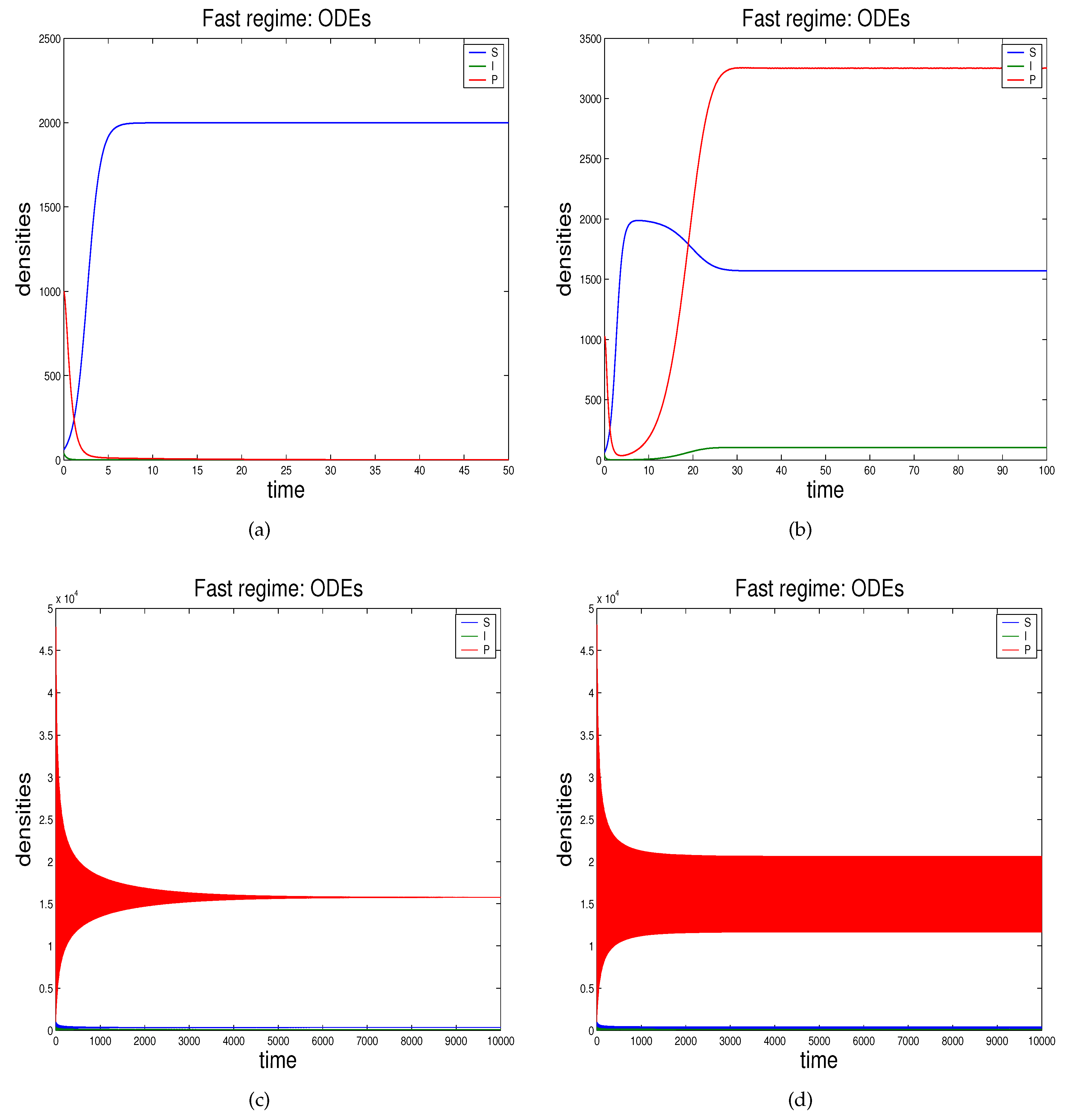
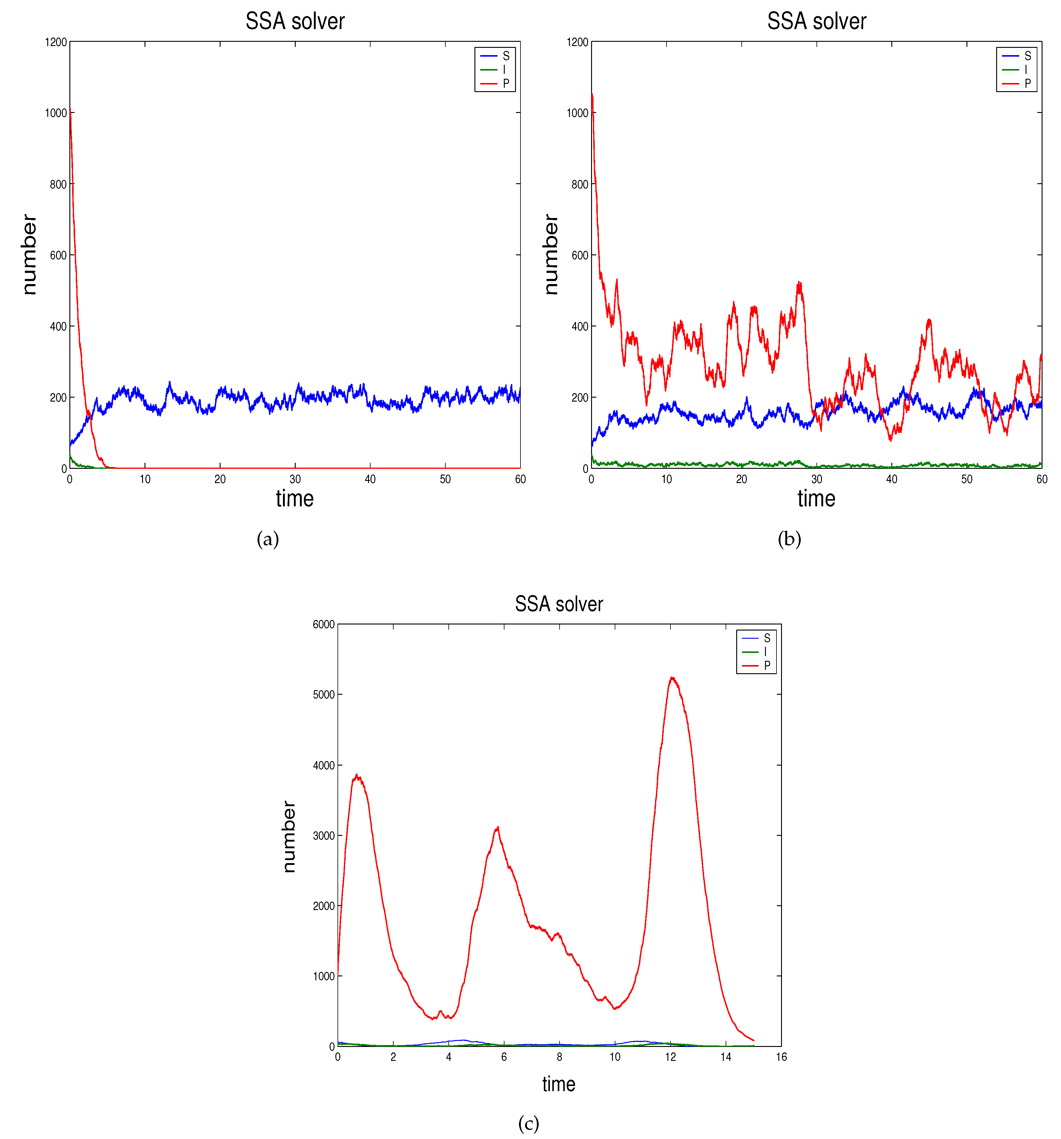
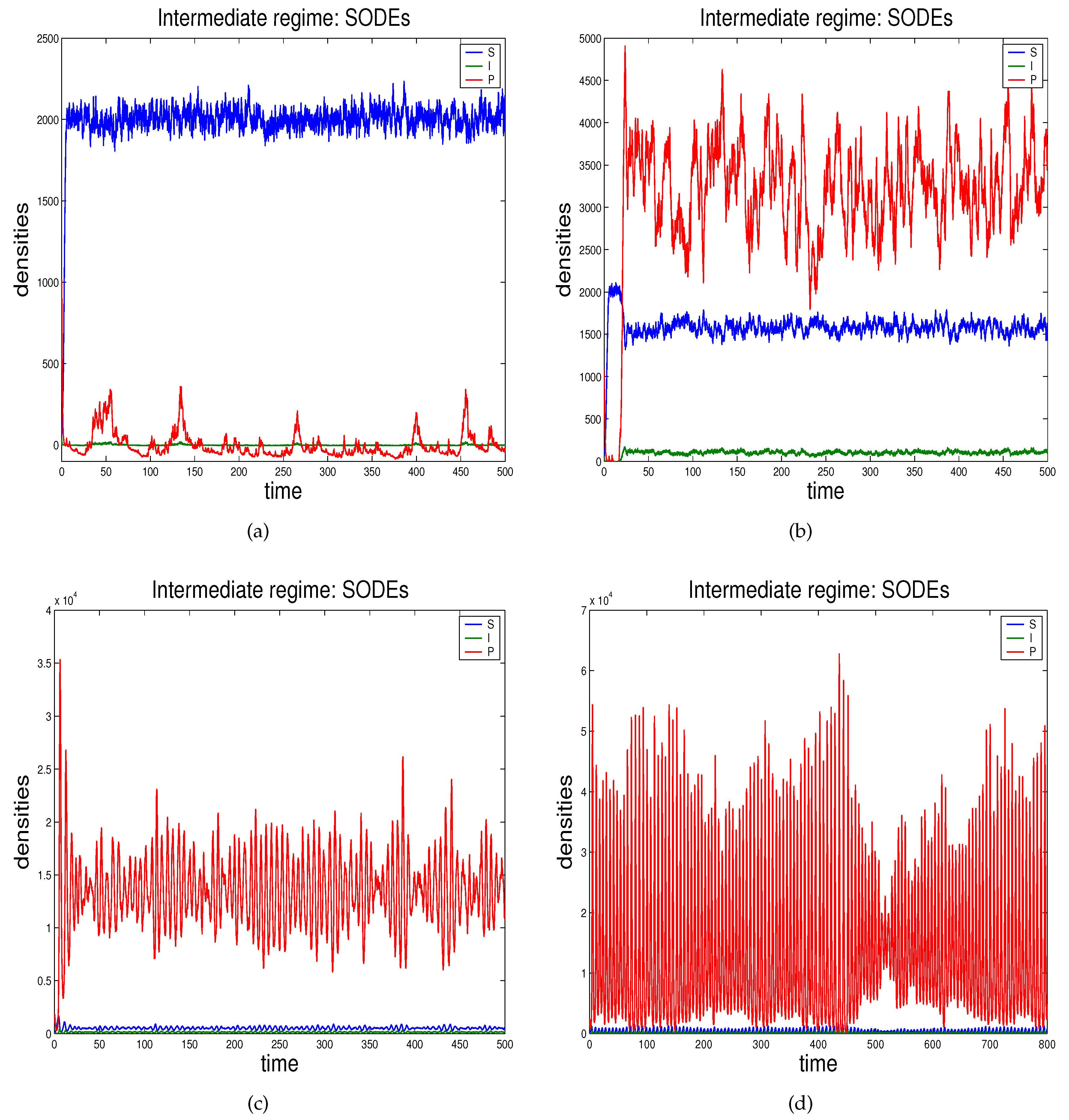
• In Section 2.3 we propose the novel technique through which we can study the effects of demographic noise in the ODEs model by Beretta and Kuang [16], going backwards to the discrete stochastic process and the continuous stochastic system (characterised by SODEs) underlying the deterministic model.

2.1. Stochastic Modeling of Genetic Regulation

In molecular biology, the general transfers describe the normal flow of biological information: DNA can be copied to DNA (DNA replication), DNA information can be copied into mRNA (messenger RNA), (transcription), and proteins can be synthesized using the information in mRNA as a template (translation).

A Genetic Regulatory Network is a collection of DNA segments in a cell that interact with each other and with other substances in the cell, thereby governing the rates at which genes in the network are transcribed into mRNA. Regulation of gene expression, or gene regulation, refers to the cellular control of the amount and timing of changes to the appearance of the functional product of a gene.

The mechanisms that act on gene expression, i.e., the ability of a gene to produce a biologically active protein, are based on biochemical processes that are inherently stochastic and are much more complex in eukaryotes than in prokaryotes. A major difference is that in eukaryotes there is the presence of the nuclear membrane, which prevents the simultaneous transcription and translation that occurs in prokaryotes [21]. Whereas, in prokaryotes, control of transcriptional initiation is the major point of regulation, in eukaryotes the regulation of gene expression can be controlled from many different points. In eukaryotes, transcriptional regulation tends to involve combinatorial interactions between several transcription factors. By “regulation” of transcription, we mean when transcription occurs and how much RNA is created.

The simulation of a discrete chemical reacting system must be done through Stochastic Simulation Algorithms (SSA), in which we assume low and integer molecular numbers. The first SSA is due to Gillespie [7] and is a rigorous procedure for numerically simulating the evolution of a set of chemical reactions in a (well-stirred) homogeneous chemical reacting system, by taking into account the randomness inherent in such a system. If $S_1,S_2,\dots ,S_N$ represent N interacting molecular species through M reaction channels, then the evolution of such a system is characterized by a discrete nonlinear Markov process in which a vector $X\left(t\right)$ of dimension N, representing numbers (integer values) of the N molecular species at time t, is evolved through time. The state vector $X\left(t\right)$ is a discrete jump Markov process, where the time evolution equation describing the probability that, given $X\left(t_0\right)=x_0$, then $X\left(t\right)=x$, i.e., $P(x,t|x_0,t_0)$ is called the Chemical Master Equation (CME) and can be written as

$$\frac{\partial }{\partial t}P(x,t|x_0,t_0)=\sum _{j=1}^M(a_j(x-{\nu }_j)P(x-{\nu }_j,t|x_0,t_0)-a_j\left(x\right)P(x,t|x_0,t_0)).$$

(1)

This discrete parabolic partial differential equation is generally too difficult to solve (either analytically or numerically) and different methods are needed to simulate its solution.

Any method to solve a system of chemical reactions is uniquely characterized by two sets of quantities: the stoichiometric vectors ${\nu }_1,\dots ,{\nu }_M$ which represent, in turn, the update of the numbers of molecules in the system if reactions $R_1,\dots ,R_M$ occur, respectively, and a set of M propensity functions $a_1\left(X\left(t\right)\right),\dots ,a_M(X\left(t\right)$, that describe the relative probabilities of reactions $R_1,\dots ,R_M$ occurring, respectively.

The SSA is an essentially exact variable time step procedure, where “exact” means that it generates the same probability distribution as the CME. At each step, two random variables are sampled from a uniform density function $U_{[0,1]}$ in order to choose which reaction will occur and what length the time step will have. The chemical species are then upgraded according to the corresponding stoichiometric vector, and the process is repeated until the simulation time range is covered. The crucial point with SSA is that the time step can become very small if the number of molecules of some reactant species is large, and it is difficult to guarantee that the simulation proceeds one reaction at a time. SSA is, thus, a computationally demanding approach that avoids its applicability when (large) reaction networks are needed to model biologically realistic phenomena.

The point with it is the multiscale nature of the underlying problem. First, some reactions are much faster than others and rapidly reach a stable state. In the SSA, the dynamics of the system are driven by the slow reactions. In a deterministic setting, this issue is called “stiffness”. Second, if some chemical species are present in relatively small quantities, then modeling by a discrete stochastic process is appropriate, whereas, if other species appear in large quantities, then stochastic or deterministic differential equations are better tools to use. In the SSA, instead, all the species are considered as discrete stochastic processes [10].

Burrage et al. [18] addressed the issue of multiscale modeling by extending the approach of Haseltine and Rawlings in [22] in classifying slow, intermediate and fast reactions to slow, intermediate, and fast regimes, resulting in a completely general, adaptive, and partitioning approach for the stochastic simulation of multiscaled systems involving chemical reactions.

Finally, the issue of non-homogeneity, typical of in vivo conditions, has been considered, among others, in the papers by Berry [23], Schnell and Turner [24], and Nicolau and Burrage [25]. All of these authors use Monte Carlo simulations on a two-dimensional lattice. In particular, Nicolau and Burrage [25] introduced the Anomalous Stochastic Simulation Algorithm (ASSA) that proved to be an effective and efficient algorithm to simulate the anomalous diffusion when the environment is not well-mixed, due to the obstacles present within the cell, such as fixed proteins or cytoskelatal structures.

However, the SSA has been successfully applied to simulate, for example, the regulation of lambda phage [26], circadian rhythms [27,28], and many other kinds of GRNs.

When noise effects are still important but continuity arguments hold, by the application of the Central Limit Theorem and by matching the first two moments of the CME, we can write an SODE that describes the continuous time evolution of the Markov process $X\left(t\right)$ involved in the SSA [29].

This equation is sometimes called the Chemical Langevin Equation (CLE) and takes the form

$$dX\left(t\right)=\sum _{j=1}^M{\nu }_j{a}_j\left(X\left(t\right)\right)dt+B\left(X\left(t\right)\right)dW\left(t\right),X\left(0\right)=X_0,$$

(2)

where $W\left(t\right)={(W_1\left(t\right),\dots ,W_N\left(t\right))}^{\prime }$ is an N dimensional vector in which its individual elements are independent Wiener processes and $B\left(X\right(t\left)\right)$ is a $N\times N$ matrix satisfying

$$B^2\left(X\left(t\right)\right)=C\left(X\left(t\right)\right)=\nu \mathrm{Diag}(a_1\left(X\left(t\right)\right),\dots ,a_M\left(X\left(t\right)\right)){\nu }^T,$$

(3)

where $\nu =[{\nu }_1,\dots ,{\nu }_M]$ is the $N\times M$ stoichiometric matrix.

Equation (2) is an It$\widehat{\mathsf{o}}$SODE representing the continuous stochastic evolution equation describing intrinsic noise.

Finally, when large numbers of molecules are taken into account so that we can talk about concentrations, the deterministic continuous setting holds. This averaged behavior is described by an ODE of initial value type of the form

$$X^{\prime }\left(t\right)=\sum _{j=1}^M{\nu }_j{a}_j\left(X\left(t\right)\right),X\left(0\right)=X_0.$$

(4)

This is the standard regime of chemical kinetics where the Law of Mass Action applies.

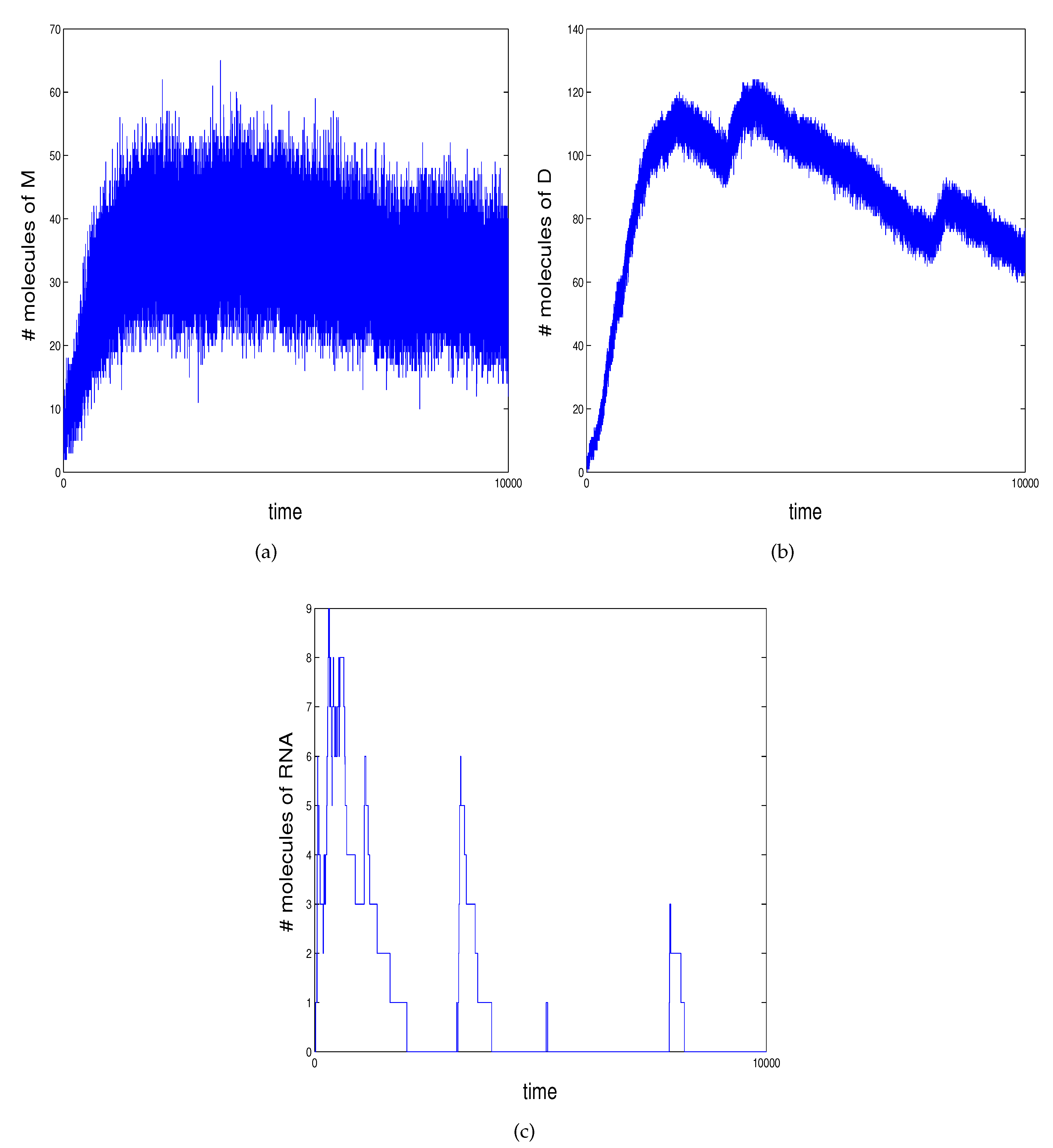
2.2. An Example of Genetic Regulation in Bacteriophage $\lambda$

A known and simple model organism is that of bacteriophage $\lambda$, which is a virus that infects the bacterium E. coli and can take two forms: lysis or lysogen. In the lysogen state, the virus replicates passively whenever E. coli replicates. Under appropriate conditions, a state change from lysogen to lysis can be induced. Many mathematical models have been developed to describe the genetic regulatory behavior of $\lambda$. These include both deterministic [30] and stochastic [26,31] kinetics models.

Most of these models consider the behavior of the $\lambda$ right operator control system and the action of regulatory proteins, CI repressor and Cro. The right operator region $O_R$ consists of three binding sites which are situated between the promoters $P_{RM}$ and $P_I$ for genes CI and Cro. The dimeric forms of repressor and Cro bind to these binding sites to regulate transcription [32]. The lysogenic state is mainly regulated by the $P_{RM}$ promoter and the CI gene, while lysis is mainly regulated by the $P_R$ promoter of the Cro gene. Shea and Ackers [33] have given a detailed model based on 40 possible configurations of $O_R$.

We consider the model introduced by Goutsias [20], based on the simplified situation of only two operating sites in $O_R$. Goutsias views this as a restricted model of the transcription regulation of the repressor protein CI in which the operator site $O_{R_1}$ is absent. The model consists of ten reactions and six unknowns: M (monomer protein), D (dimer transcription factor), RNA (mRNA produced by transcription), DNA (free of dimers), DNA1 (bound by D at binding site $O_{R_1}$), and DNA2 (bound at sites $O_{R_1}$ and $O_{R_2}$).

The network can be described by the following reactions:

$$\begin{array}{ccc}\hfill DNA1& \to & RNA+DNA1\hfill \\ \hfill RNA& \to & RNA+M\hfill \\ \hfill M& \to & 0\hfill \\ \hfill RNA& \to & 0\hfill \\ \hfill M+M& \to & D\hfill \\ \hfill D& \to & M+M\hfill \\ \hfill DNA+D& \to & DNA1\hfill \\ \hfill DNA1& \to & DNA+D\hfill \\ \hfill DNA1+D& \to & DNA2\hfill \\ \hfill DNA2& \to & DNA1+D,\hfill \end{array}$$

(5)

where

• reaction 1 models transcription to mRNA occurring when D occupies $O_{R_1}$;
• reactions $2,3,4$ model mRNA translated into proteins and the decay of both;
• reaction 5 models protein dimerizing to the transcription factor D;
• reactions $6,7,8$ model activation of transcription of M when D binds at $O_{R_1}$;
• reactions 9 and 10 model prevention of the RNA polymerase from binding at the promoter region and repression of transcription when D binds at $O_{R_2}$.

The rate constant corresponding to reaction j is denoted by $c_j$.

According to the method used in [17] for modeling first order, second order, and homodimeric reactions, we use variables $X_i\left(t\right),i=1,\dots ,6$, to characterize the molecular state of the transcriptional regulatory system at time $t\ge 0$, where $X_i\left(t\right)=(M,D,RNA,DNA,DNA1,DNA2)$. From the Goutsias model (5), we obtain the following propensity functions $a_j\left(X\right)),j=1,\dots ,10$, and the stoichiometric vectors ${\nu }_j,j=1,\dots ,10$

$$\begin{array}{ccc}{a}_1\left(X\right)\hfill & =\hfill & c_1{X}_5\hfill \\ a_2\left(X\right)\hfill & =\hfill & c_2{X}_3\hfill \\ a_3\left(X\right)\hfill & =\hfill & c_3{X}_1\hfill \\ a_4\left(X\right)\hfill & =\hfill & c_4{X}_3\hfill \\ a_5\left(X\right)\hfill & =\hfill & c_5{X}_1^2\hfill \\ a_6\left(X\right)\hfill & =\hfill & c_6{X}_2\hfill \\ a_7\left(X\right)\hfill & =\hfill & c_7{X}_2{X}_4\hfill \\ a_8\left(X\right)\hfill & =\hfill & c_8{X}_5\hfill \\ a_9\left(X\right)\hfill & =\hfill & c_9{X}_2{X}_5\hfill \\ a_{10}\left(X\right)\hfill & =\hfill & c_{10}{X}_6\hfill \end{array}\begin{array}{ccc}{\nu }_1\hfill & =\hfill & [0,0,1,0,0,0]\hfill \\ {\nu }_2\hfill & =\hfill & [1,0,0,0,0,0]\hfill \\ {\nu }_3\hfill & =\hfill & [-1,0,0,0,0,0]\hfill \\ {\nu }_4\hfill & =\hfill & [0,0,-1,0,0,0]\hfill \\ {\nu }_5\hfill & =\hfill & [-2,1,0,0,0,0]\hfill \\ {\nu }_6\hfill & =\hfill & [2,-1,0,0,0,0]\hfill \\ {\nu }_7\hfill & =\hfill & [0,-1,0,-1,1,0]\hfill \\ {\nu }_8\hfill & =\hfill & [0,1,0,1,-1,0]\hfill \\ {\nu }_9\hfill & =\hfill & [0,-1,0,0,-1,1]\hfill \\ {\nu }_{10}\hfill & =\hfill & [0,1,0,0,1,-1].\hfill \end{array}$$

(6)

We initialize the system with $m\ge 1$ monomers and $d\ge 1$ dimers, and we assume $g\ge 1$ DNA templates per cell. In this case, we have the initial state vector

$$X_0=(m,d,0,g,0,0).$$

(7)

The values of the specific probability rate constants $c_j$ in (6) are taken from relevant papers (see [20] and references therein) and are listed below:

$$\begin{array}{ccc}{c}_1\hfill & =\hfill & 0.078\hfill \\ c_2\hfill & =\hfill & 0.043\hfill \\ c_3\hfill & =\hfill & 0.0007\hfill \\ c_4\hfill & =\hfill & 0.0039\hfill \\ c_5\hfill & =\hfill & 0.05\ast {10}^9/AV\hfill \\ c_6\hfill & =\hfill & 0.5\hfill \\ c_7\hfill & =\hfill & 0.012\ast {10}^9/AV\hfill \\ c_8\hfill & =\hfill & 0.4791\hfill \\ c_9\hfill & =\hfill & 0.00012\ast {10}^9/AV\hfill \\ c_{10}\hfill & =\hfill & 0.00021969,\hfill \end{array}$$

(8)

where $A=6.0221415\ast {10}^{23}{mol}^{-1}$ is the Avogadro number and V is the volume that, for simplicity, we assume constant and equal to ${10}^{-15}$. We set $m=2$, $d=6$, and assume that an average E. coli cell is infected by about two $\lambda$ chromosomes, i.e., $g=2$.

For simulating the solution of the Goutsias discrete model (5), we used an enhancement of the Gillespie SSA developed by the Kevin Burrage’s team in the years 2004–2006 (K.B, Tianhai Tian, Manuel Barrio, André Leier, Tatiana Marquez-Lago, and the first author of this paper) using a “sorting” algorithm, from now on addressed as the “sorting SSA”, that allows the speeding up of the performance of the algorithm when choosing what reaction number should take place at every time step and uses a special time stepsize for monitoring and storing the updated concentrations of species [34].

We recall that, in a stochastic setting, we can provide either single simulations of just one strong solution over a given path, or a number of independent simulations in order to collect information about mean behaviors. Since individual solutions are, however, representative of the dynamics of the processes being modeled, in Figure 1 that follow we will show single simulations of one strong solution.

2.3. Demographic Noise in Bacteriophage Infections: The Backward Gene Regulation Approach

Demographic noise in population dynamics and epidemic models has been studied by many authors with different approaches [5,14,35,36,37,38]. As already mentioned in the previous sections, in all of these approaches the starting system is discrete. Now, suppose we have an ODE model of different kinds (biological, ecological, biochemical, etc.), and we wish to address the issue of how demographic noise affects the underlying interacting species, in order to capture the intrinsic variability neglected by the deterministic modeling. We consider the ODE model describing the dynamics of epidemics induced by bacteriophages in marine bacteria populations, introduced by Beretta and Kuang in [16].

The model equations are

$$\begin{array}{ccc}{\displaystyle \frac{dS\left(t\right)}{dt}}\hfill & =\hfill & \alpha S\left(t\right)\left({\displaystyle 1-\frac{S\left(t\right)+I\left(t\right)}{C}}\right)-KS\left(t\right)P\left(t\right)\hfill \\ {\displaystyle \frac{dI\left(t\right)}{dt}}\hfill & =\hfill & KS\left(t\right)P\left(t\right)-\lambda I\left(t\right)\hfill \\ {\displaystyle \frac{dP\left(t\right)}{dt}}\hfill & =\hfill & -KS\left(t\right)P\left(t\right)-\mu P\left(t\right)+b\lambda I\left(t\right),\hfill \end{array}$$

(9)

where $S\left(t\right)$ is the fraction of total bacteria population susceptible of being infected at time t, $I\left(t\right)$ is the fraction of infected bacteria at time t, $P\left(t\right)$ are the (virulent) phage at time t, $\alpha >0$ is the bacteria intrinsic birth rate constant, $C>0$ is the bacteria carrying capacity, $K>0$ is the effective per bacteria contact rate constant with viruses, $\lambda >0$ is the lysis death rate constant, and $\mu >0$ is the viruses death rate constant. Parameter $b>1$ is the virus replication factor.

The initial condition for system (9) is any point in

$${\mathbb{R}}_{+0}^3=\left\{(S,I,P)\in {\mathbb{R}}^3|S\ge 0,I\ge 0,P\ge 0\right\}.$$

By rescaling the variables on the carrying capacity C and introducing the dimensionless time $\tau =KCt$, we obtain the dimensionless model equations

$$\begin{array}{ccc}{\displaystyle \frac{ds\left(\tau \right)}{d\tau }}\hfill & =\hfill & as\left(\tau \right)\left[1-\left(i\right(\tau )+s(\tau \left)\right)\right]-s\left(\tau \right)p\left(\tau \right)\hfill \\ {\displaystyle \frac{di\left(\tau \right)}{d\tau }}\hfill & =\hfill & s\left(\tau \right)p\left(\tau \right)-li\left(\tau \right)\hfill \\ {\displaystyle \frac{dp\left(\tau \right)}{d\tau }}\hfill & =\hfill & -s\left(\tau \right)p\left(\tau \right)-m_{p}p\left(\tau \right)+bli\left(\tau \right),\hfill \end{array}$$

(10)

where

$$a=\frac{\alpha }{KC},l=\frac{\lambda }{KC},m_p=\frac{\mu }{KC}$$

(11)

are the dimensionless parameters. In the simplified dimensionless form (10) the main mathematical features of model (9) were analyzed in [16]. The parameter $b\in (l,+\infty )$ was chosen as the parameter on which the dynamics of the infection depends, due to the fact that viral infection induces bacterial lysis, thus releasing, on average, b viruses for each infected bacterium into the marine environment. Beretta and Kuang proved that there exists a threshold value for b beyond which the (positive) endemic equilibrium bifurcates from the free disease one. In turn, for large values of b, the endemic equilibrium bifurcates toward a periodic solution. Model (9) was a seminal study for a quantity of other models, either deterministic or stochastic. Authors have also taken into account the influence of time delay, either discrete or distributed delay, resulting in delay differential equations (DDEs) or stochastic delay differential equations (SDDEs) [39,40,41,42,43,44,45,46].

We now view the Beretta and Kuang model (9) as the deterministic counterpart of the CLE associated with the discrete stochastic phenomenon, that is the bacteriophage infection on “units” of marine bacteria, under the effect of demographic noise. In other words, we consider the ODE model as the $\mathsf{\Delta }t\to 0$ limit of a jump Markov process $X\left(t\right)=(X_1\left(t\right),X_2\left(t\right),X_3\left(t\right))$, where

$$X_1\left(t\right)=S\left(t\right),X_2\left(t\right)=I\left(t\right),X_3\left(t\right)=P\left(t\right),$$

satisfying system (9). The initial number of units of the single interacting species (susceptible and infected bacteria and phages) is assumed to be large.

By multiplying $S\left(t\right)$ by the terms within parentheses in the first equation of model (9), we observe that seven reactions are taking place:

$$\begin{array}{ccc}\hfill S& \to & S\hfill \\ \hfill S+S& \to & 0\hfill \\ \hfill S+I& \to & I\hfill \\ \hfill S+P& \to & I\hfill \\ \hfill I& \to & 0\hfill \\ \hfill P& \to & P\hfill \\ \hfill I& \to & P.\hfill \end{array}$$

(12)

The associate propensity functions $a_j\left(X\right)$, the stoichiometric vectors ${\nu }_j$, and reaction rates $c_j$ are

$$\begin{array}{ccc}{a}_1\left(X\right)\hfill & =\hfill & c_1{X}_1\hfill \\ a_2\left(X\right)\hfill & =\hfill & c_2{X}_1^2\hfill \\ a_3\left(X\right)\hfill & =\hfill & c_3{X}_1{X}_2\hfill \\ a_4\left(X\right)\hfill & =\hfill & c_4{X}_1{X}_3\hfill \\ a_5\left(X\right)\hfill & =\hfill & c_5{X}_2\hfill \\ a_6\left(X\right)\hfill & =\hfill & c_6{X}_3\hfill \\ a_7\left(X\right)\hfill & =\hfill & c_7{X}_2\hfill \end{array}\begin{array}{ccc}{\nu }_1\hfill & =\hfill & [1,0,0]\hfill \\ {\nu }_2\hfill & =\hfill & [-2,0,0]\hfill \\ {\nu }_3\hfill & =\hfill & [-1,0,0]\hfill \\ {\nu }_4\hfill & =\hfill & [-1,1,-1]\hfill \\ {\nu }_5\hfill & =\hfill & [0,-1,0]\hfill \\ {\nu }_6\hfill & =\hfill & [0,0,-1]\hfill \\ {\nu }_7\hfill & =\hfill & [0,0,1]\hfill \end{array}\begin{array}{ccc}{c}_1\hfill & =\hfill & \alpha \hfill \\ c_2\hfill & =\hfill & \frac{\alpha }{2C}\hfill \\ c_3\hfill & =\hfill & \frac{\alpha }{C}\hfill \\ c_4\hfill & =\hfill & K\hfill \\ c_5\hfill & =\hfill & \lambda \hfill \\ c_6\hfill & =\hfill & \mu \hfill \\ c_7\hfill & =\hfill & b\lambda .\hfill \end{array}$$

(13)

Moreover, we know that the Chemical Langevin Equation associated to the discrete system (13) takes the form:

$$dX\left(t\right)=\sum _{j=1}^7{\nu }_j{a}_j\left(X\left(t\right)\right)dt+B\left(X\left(t\right)\right)dW\left(t\right),X\left(0\right)=X_0,$$

(14)

where $W\left(t\right)={(W_1\left(t\right),\dots ,W_N\left(t\right))}^{\prime }$ is a $3-$dimensional vector whose individual elements are independent Wiener processes and $B\left(X\right(t\left)\right)$ is a $3\times 3$ matrix satisfying

$$B^2\left(X\left(t\right)\right)=C\left(X\left(t\right)\right)=\nu \mathrm{Diag}(a_1\left(X\left(t\right)\right),\dots ,a_7\left(X\left(t\right)\right)){\nu }^T,$$

(15)

where $\nu =[{\nu }_1,\dots ,{\nu }_7]$ is a $3\times 7$ stoichiometric matrix. We recall that Equation (14) is an It$\widehat{\mathsf{o}}$SODE and represents the continuous stochastic evolution equation modeling demographic (intrinsic) noise within system (12).

Using formulas (13), in Equation (14), matrix computations show that the $3\times 7$ stoichiometric matrix C, satisfying $B^2\left(X\left(t\right)\right)=C\left(X\left(t\right)\right)=\nu \mathrm{Diag}(a_1\left(X\left(t\right)\right),\dots ,a_7\left(X\left(t\right)\right)){\nu }^T$ and $\nu =[{\nu }_1,\dots ,{\nu }_7]$ (where $B\left(X\right(t\left)\right)$ is a $3\times 3$ matrix), is

$$C=\left(\begin{array}{ccc}{a}_1+4a_2+a_3+a_4& -a_4& a_4\\ -a_4& a_4+a_5& -a_4\\ a_4& -a_4& a_4+a_6+a_7\end{array}\right).$$

(16)

All the numerical experiments presented in this paper were done on a last generation PC and coded in MATLAB (R2019a) environment running under Windows 10.

3. Results

A thorough discussion of the analytical properties of the Beretta and Kuang ODEs model (9), including existence and uniqueness of the solution and the dependence of the dynamics of the model on the phage replication number b, can be found in [16]. For our purposes, using a standard ODEs method for non-stiff differential equations, the simulations of the solution in continuous deterministic setting result in Figure 2. Figure 2a shows that, if b is less than the critical value $b^{\ast }\approx 16$, only the boundary equilibrium $E_f=(C,0,0)$ exists. Susceptible bacteria reach their maximum value, while infected bacteria and phage vanish. Figure 2b,c show that for $b^{\ast }<b<b_c$, where a second critical value $b_c\approx 95$, a globally stable positive equilibrium $E_{+}=(S^{\ast },I^{\ast },P^{\ast })$ exists, thus providing coexistence of bacteria and phage. As a last case, Figure 2d shows that when $b>b_c$, where $b_c$ is the bifurcation value, then a positive equilibrium exists but is unstable.

If we apply the backward method described in Section 2.3 to the ODEs model (9), we obtain the discrete stochastic system (12) and (13) modeling demographic noise in the phage-bacteria interaction and simulate the solutions via the sorting SSA. We expect that the more parameter b increases, the more the dynamics of the discrete system (12) and (13) is modified, accordingly to the continuous case. Figure 3 shows that the solutions fluctuate much more randomly with respect to the continuous model, particularly in the wide range of parameter b providing coexistence of the two species, i.e., $b^{\ast }<b<b_c$ (Figure 3b) and with respect to the phage population. Moreover, we note that the order of the solutions, whatever b is, diminish by one when we turn from “concentrations” (continuous deterministic case) to “integer number of individuals” (discrete stochastic case).

The simulations of system (12) and (13) with the SSA solver is, however, slow; thus, the integration time is much shorter than the integration time reached for the fast modeling regime via the ODE system (9). So, if we wish to know the long-time behavior of the stochastic biological system, we have to consider the continuous stochastic regime represented by the It$\widehat{\mathsf{o}}$SODE (14). Using the Euler-Maruyama method for SODEs [41], we obtained Figure 4 confirming that even in the long-time behavior parameter b is crucial: for low values of b, the solution still goes to the corresponding equilibrium state (Figure 4a), although more randomly than in the deterministic setting. For higher values of b the effects of demographic noise, especially for the phage population, are much more evident: the positive equilibrium $E_{+}=(S^{\ast },I^{\ast },P^{\ast })$ becomes unstable for values of parameter b much smaller than the deterministic bifurcation value $b_c=94.451$ (Figure 4b,c).

We also note that the order of the solutions, for all values of parameter b, increases by one with respect to the discrete stochastic case, thus regaining the same order of the original continuous, though deterministic, setting.

4. Discussion

In this article, we provided a method to offer insights into deterministic differential models when intrinsic noise is of interest. If the ordinary differential system is of biological or ecological nature, intrinsic noise is the so-called demographic noise. Our framework is that of chemical kinetics used to model intrinsic noise involved in molecular biology, in particular, in genetic regulation using SSAs. We first gave an example of application of the direct method for modeling demographic noise to a gene regulation network in bacteriophage $\lambda$, using a particular type of SSA developed by Burrage et al. in [17,34,47]. Next, we inferred the effects of demographic noise on an ODEs model of phage-bacteria interaction [16] going backward from the deterministic differential system to its discrete stochastic counterpart, thus giving insights to the effects of randomly fluctuating birth and death rates, immigration and/or emigration of the involved molecular species. We observe that our method is quite general and can be applied to ODE models of different nature, not only in life sciences. Unfortunately, at the moment its applicability is limited to ODEs where the underlying chemical reaction channels are either first order, heterodimeric (second and higher order), homodimeric, and Hill-type reactions for which a mathematical formulation can be provided, according to [17,19].

We are not able to compare our results with other authors’ results since, to our knowledge, no equivalent methods starting from the deterministic setting can be found in the literature. Nevertheless, it would be interesting to compare the outcomes of our backward method with those obtained by applying the direct method to the same biological process in such a way to evaluate the robustness of the backward technique. We expect that the two approaches (direct and inverse) lead to very similar outcomes. Finally, a higher level of biological realism could be reached if, jointly with demographic noise, we consider time delay, for example, for modeling incubation time or latency period. In such a case, for the direct method, the Delay Stochastic Simulation Algorithm (DSSA) and the Delay Chemical Master Equation [15,34,48] would be the appropriate simulation tools to use. As with the backward (delay) method, there are good models to start with, for example, the Beretta and Kuang or the Beretta et al. [39,49] phage infection models with delay. All of these issues are being addressed in a new research article in preparation.

References

1. Mao, X. Stochastic stabilization and destabilization. Syst. Control Lett. 1994, 23, 279–290. [Google Scholar] [CrossRef]
2. Mao, X. Stochastic self-stabilization. Stoch. Stoch. Rep. 1996, 57, 57–70. [Google Scholar] [CrossRef]
3. Mao, X. Some contributions to stochastic asymptotic stability and boundedness via multiple Lyapunov functions. J. Math. Anal. Appl. 2001, 153, 325–340. [Google Scholar] [CrossRef] [Green Version]
4. Elowitz, M.B.; Levine, A.J.; Siggia, E.D.; Swain, P.S. Stochastic gene expression in a single cell. Science 2002, 297, 1183–1186. [Google Scholar] [CrossRef] [PubMed] [Green Version]
5. Allen, L.J.S. An Introduction to Stochastic Processes with Applications to Biology, 2nd ed.; Chapman Hall/CRC Press: Boca Raton, FL, USA, 2003. [Google Scholar]
6. Allen, L.J.S. Stochastic Population and Epidemic Models. Persistence and Extinction; Mathematical Biosciences Lecture Series, Stochastics in Biological Systems; Springer: New York, NY, USA, 2015; Volume 1.3. [Google Scholar]
7. Gillespie, D.T. A general method for numerically simulating the stochastic time evolution of coupled chemical reactions. J. Comput. Phys. 1976, 22, 403–434. [Google Scholar] [CrossRef]
8. Gillespie, D.T. Approximate accelerated stochastic simulation of chemically reacting systems. J. Chem. Phys. 2001, 115, 1716. [Google Scholar] [CrossRef]
9. Tian, T.; Burrage, K. Binomial leap methods for simulating stochastic chemical kinetics. J. Chem. Phys. 2004, 121, 10356–10364. [Google Scholar] [CrossRef] [Green Version]
10. Cao, Y.; Li, H.; Petzold, L. Efficient formulation of the stochastic simulation algorithm for chemically reacting systems. J. Chem. Phys. 2004, 121, 4059–4067. [Google Scholar] [CrossRef]
11. Cao, Y.; Gillespie, D.T.; Petzold, L.R. Avoiding negative populations in explicit Poisson tau-leaping. J. Chem. Phys. 2005, 123, 054104. [Google Scholar] [CrossRef] [Green Version]
12. Cao, Y.; Gillespie, D.T.; Petzold, L.R. Efficient step size selection for the tau-leaping simulation method. J. Chem. Phys. 2006, 124, 044109. [Google Scholar] [CrossRef]
13. Smith, H.L.; Trevino, R.T. Bacteriophage Infection Dynamics: Multiple Host Binding Sites. Math. Model. Nat. Phenom. 2009, 4, 109–134. [Google Scholar] [CrossRef] [Green Version]
14. Mandal, P.S.; Allen, L.J.S.; Banerjee, M. Stochastic modeling of phytoplankton allelopathy. Appl. Math. Model. 2014, 38, 1583–1596. [Google Scholar] [CrossRef]
15. Carletti, M.; Montani, M.; Meschini, V.; Radici, L.; Bianchi, M. Stochastic modeling of PTEN regulation in brain tumors. A model for glioblastoma multiforme. Math. Biosci. Eng. 2015, 12, 965–981. [Google Scholar] [PubMed]
16. Beretta, E.; Kuang, Y. Modeling and analysis of a marine bacteriophage infection. Math. Biosci. 1998, 149, 57–76. [Google Scholar] [CrossRef]
17. Burrage, K.; Tian, T. Effective simulation techniques for biological systems, in fluctuations and noise in biological, biophysical, and biomedical systems II. In Proceedings of the SPIE—The International Society for Optical Engineering: Fluctuations and Noise in Biological, Biophysical, and Biomedical Systems II, Maspalomas, Spain, 26–28 May 2004; SPIE: Bellingham, WA, USA, 2004; Volume 5467, pp. 311–325. [Google Scholar]
18. Burrage, K.; Tian, T.; Burrage, P.M. A multi-scaled approach for simulating chemical reaction systems. Prog. Biophys. Mol. Biol. 2004, 85, 217–234. [Google Scholar] [CrossRef]
19. Burrage, K.; Burrage, P.; Leier, A.; Marquez-Lago, T.A.; Marquez-Lago, T. A review of stochastic and delay simulation approaches in both time and space in computational cell biology. In Stochastic Processes, Multiscale Modeling, and Numerical Methods for Computational Cellular Biology; Holcman, D., Ed.; Springer: New York, NY, USA, 2017. [Google Scholar]
20. Goutsias, J. Quasiequilibrium approximation of fast reaction kinetics in stochastic biochemical sysmtems. J. Chem. Phys. 2005, 122, 184102. [Google Scholar] [CrossRef] [Green Version]
21. Choudhuri, S. Gene Regulation and Molecular Toxicology. Toxicol. Mech. Methods 2004, 15, 1–23. [Google Scholar] [CrossRef]
22. Haseltine, E.L.; Rawlings, J.B. Approximate simulation of coupled fast and slow reactions for stochastic chemical kinetics. J. Chem. Phys. 2002, 117, 6959–6969. [Google Scholar] [CrossRef] [Green Version]
23. Berry, H. Monte-Carlo simulations of enzyme reactions in two dimensions: Fractal kinetics and spatial segregation. Biophys. J. 2002, 83, 1891–1901. [Google Scholar] [CrossRef] [Green Version]
24. Schnell, S.; Turner, T.E. Reaction kinetics in Intracellular environments with macromolecular crowding: Simulations and rate laws. Prog. Biophysica Mol. Biol. 2004, 85, 235–260. [Google Scholar] [CrossRef]
25. Nicolau, D.V., Jr.; Burrage, K. Stochastic simulation of chemical reactions in spatially complex media. Comput. Math. Appl. 2008, 55, 1007–1018. [Google Scholar] [CrossRef]
26. Arkin, A.; Ross, J.; McAdams, H.H. Stochastic kinetic analysis of developmental pathway bifurcation in phage lambda-infected Escherichia coli cells. Genetics 1998, 149, 1633–1648. [Google Scholar] [PubMed]
27. Elowitz, M.B.; Leibler, S. A synthetic oscillatory network of transcriptional regulators. Nature 2000, 403, 335–338. [Google Scholar] [CrossRef] [PubMed]
28. Gonze, D.; Halloy, J.; Goldbeter, A. Robustness of circadian rythms with respect to molecular noise. Proc. Natl. Acad. Sci. USA 2002, 99, 673–678. [Google Scholar] [CrossRef] [Green Version]
29. Gillespie, D.T. A rigorous derivation of the chemical master equation. Physica A 1992, 188, 404–425. [Google Scholar] [CrossRef]
30. Ackers, G.K.; Johnson, A.D.; Shea, M.A. Quantitative model for gene regulation by λ phage repressor. Proc. Natl. Acad. Sci. USA 1982, 79, 1129–1133. [Google Scholar] [CrossRef] [Green Version]
31. Hasty, J.; Pradines, J.; Dolnik, M.; Collins, J.J. Noise-based switches and amplifiers for gene expression. Proc. Natl. Acad. Sci. USA 2000, 97, 2075–2080. [Google Scholar] [CrossRef] [Green Version]
32. Ptashne, M. A Genetic Switch: Phage λ Revisited, 3rd ed.; Cold Spring Harbor Laboratory Press: Cold Spring Harbor, NY, USA, 2004. [Google Scholar]
33. Shea, M.A.; Ackers, G.K. The OR control system of bacteriophage Lambda: A physical-chemical model for gene regulation. J. Mol. Biol. 1985, 181, 211–230. [Google Scholar] [CrossRef]
34. Barrio, M.; Burrage, K.; Leier, A.; Tian, T. Oscillatory Regulation of Hes1: Discrete stochastic delay modeling and simulation. PLoS Comput Biol. 2006, 2, e117. [Google Scholar] [CrossRef] [Green Version]
35. Braumann, C.A. Environmental versus demographic stochasticity in population growth. In Workshop on Branching Processes and Their Applications; González, M.V., Puerto, I.M., Martínez, R., Molina, M., Mota, M., Ramos, A., Eds.; 37 Lecture Notes in Statistics—Proceedings; Springer: Berlin/Heidelberg, Germany, 2010; Volume 197. [Google Scholar]
36. Vieira dos Santos, R. Discreteness inducing coexistence. Physica A 2013, 392, 5888–5897. [Google Scholar] [CrossRef] [Green Version]
37. Constable, G.W.A.; Rogers, T.; McKane, A.J.; Tarnita, C.E. Demographic noise can reverse the direction of deterministic selection. Proc. Natl. Acad. Sci. USA 2016, 113, E4745–E4754. [Google Scholar] [CrossRef] [PubMed] [Green Version]
38. Weissmann, H.; Shnerb, N.M.; Kessler, D.A. Simulation of spatial systems with demographic noise. Phys. Rev. E 2018, 98, 022131. [Google Scholar] [CrossRef] [PubMed] [Green Version]
39. Beretta, E.; Kuang, Y. Modeling and analysis of a marine bacteriophage infection with latency period. Nonlin. Anal. RWA 2001, 2, 35–74. [Google Scholar] [CrossRef]
40. Rabinovitch, A.; Aviramb, I.; Zaritsky, A. Bacterial debris—An ecological mechanism for coexistence of bacteria and their viruses. J. Theor. Biol. 2003, 224, 377–383. [Google Scholar] [CrossRef]
41. Buckwar, E. The Θ-Maruyama scheme for stochastic functional differential equations with distributed memory term. Monte Carlo Methods Appl. 2004, 10, 235–244. [Google Scholar] [CrossRef]
42. Gourley, S.A.; Kuang, Y. A stage structured predator-prey model and its dependence on maturation delay and death rate. J. Math. Biol. 2004, 49, 188–200. [Google Scholar] [CrossRef]
43. Gourley, S.A.; Kuang, Y. A delay reaction-diffusion model of the spread of bacteriophage infection. SIAM J. Appl. Math. 2005, 65, 550–566. [Google Scholar] [CrossRef] [Green Version]
44. Liu, S.; Liu, Z.; Tang, J. A delayed marine bacteriophage infection model. Appl. Math. Lett. 2007, 20, 702–706. [Google Scholar] [CrossRef] [Green Version]
45. Carletti, M. On the stability properties of a stochastic model for phage–bacteria interaction in open marine environment. Math. Biosci. 2002, 175, 117–131. [Google Scholar] [CrossRef]
46. Carletti, M. Mean-square stability of a stochastic model for bacteriophage infection with time delays. Math. Biosci. 2007, 210, 395–414. [Google Scholar] [CrossRef]
47. Leier, A.; Marquez-Lago, T.T.; Burrage, K. Generalized binomial Tau-leap method for biochemical kinetics incorporating both delay and intrinsic noise. J. Chem. Phys. 2008, 128, 205107. [Google Scholar] [CrossRef] [PubMed] [Green Version]
48. Tian, T.; Burrage, K.; Burrage, P.M.; Carletti, M. Stochastic delay differential equations for genetic regulatory networks. J. Comp. Appl. Math. 2007, 205, 696–707. [Google Scholar] [CrossRef]
49. Beretta, E.; Carletti, M.; Solimano, F. On the effects of environmental fluctuations in a simple model of bacteria-bacteriophage interaction. Canad. Appl. Math. Quart. 2000, 8, 321–366. [Google Scholar]
Figure 1. Numerical simulations of the first three components of solution state vector X ( t ) of the Goutsias model (5) via the sorting Stochastic Simulation Algorithm (SSA). (a) M ( t ) , (b) D ( t ) and (c) R N A ( t ) (Time in minutes in the horizontal axis; number of molecules in the vertical axis).
Mathematics 07 01204 g001
Figure 2. Plots of the solution state vector ( S ( t ) , I ( t ) , P ( t ) ) (time in days in the horizontal axis; u n i t s v o l u m e 1 , volume in c m 3 , in the vertical axis) of the Beretta and Kuang ODEs model (9) for different values of parameter b. (a) b = 15 , (b) b = 20 , (c) b = 94 , and (d) b = 95 .
Mathematics 07 01204 g002
Figure 3. Plots of the solution state vector ( S ( t ) , I ( t ) , P ( t ) ) (time in days in the horizontal axis; u n i t s v o l u m e 1 , volume in c m 3 , in the vertical axis) of the discrete phage-bacteria model in Equations (12) and (13), obtained by the sorting SSA for different values of parameter b. (a) b = 15 , (b) b = 20 , and (c) b = 95 .
Mathematics 07 01204 g003
Figure 4. Plots of one path of the solution ( S ( t ) , I ( t ) , P ( t ) ) (time in days in the horizontal axis; u n i t s v o l u m e 1 , volume in c m 3 , in the vertical axis) of the SODEs model (14)–(16), obtained from the discrete stochastic Goutsias model (5) when modeling demographic noise for different values of parameter b. (a) b = 15 , (b) b = 20 , (c) b = 60 , and (d) b = 95 . The Euler-Maruyama method is used.
Mathematics 07 01204 g004