Local Convergence and Attraction Basins of Higher Order, Jarratt-Like Iterations

Abstract

We studied the local convergence of a family of sixth order Jarratt-like methods in Banach space setting. The procedure so applied provides the radius of convergence and bounds on errors under the conditions based on the first Fréchet-derivative only. Such estimates are not proposed in the approaches using Taylor expansions of higher order derivatives which may be nonexistent or costly to compute. In this sense we can extend usage of the methods considered, since the methods can be applied to a wider class of functions. Numerical testing on examples show that the present results can be applied to the cases where earlier results are not applicable. Finally, the convergence domains are assessed by means of a geometrical approach; namely, the basins of attraction that allow us to find members of family with stable convergence behavior and with unstable behavior.

1. Introduction

We provide local criteria for finding a unique solution $\delta$ of the nonlinear equation

$$H\left(x\right)=0,$$

(1)

for Banach space valued mappings with $H:D\subseteq X\to Y$, and H is differentiable according to Fréchet [1,2]. Many authors have studied local and semilocal convergence criteria of iterative methods (see, for example [3,4,5,6,7,8,9,10,11,12,13,14]).

The most well-known iterative method for approximating a solution $\delta$ of Equation (1) is Newton’s method, which is given by

$$x_{n+1}=x_n-H^{\prime }{\left(x_n\right)}^{-1}H\left(x_n\right),\mathrm{for}\mathrm{each}n=0,1,2,\dots ,$$

(2)

which has a quadratic order of convergence. In order to achieve higher convergence order, a number of modified, multistep Newton’s or Newton-type iterations have been developed in the literature; see [3,4,6,7,9,10,11,12,15,16,17,18,19] and references cited therein.

There is another important class of multistep methods based on Jarratt methods or Jarratt-type methods [20,21,22]. Such methods have been extensively studied in the literature; see [23,24,25,26,27,28] and references therein. In particular, Alzahrani et al. [23] have recently proposed a class of sixth order methods for approximating solution of $H\left(x\right)=0$ using a Jarratt-like composite scheme. These methods are very attractive and their local convergence analysis is worthy of study. The authors have shown some important special cases of the class which are defined for each $n=0,1,2,\cdots$ by

Method-I:

$$\left\{\begin{array}{c}{y}_n=x_n-\frac{2}{3}{H}^{\prime }{\left(x_n\right)}^{-1}H\left(x_n\right),\hfill \\ z_n=x_n-\left[\left(12{(H^{\prime }\left(x_n\right)+H^{\prime }\left(y_n\right))}^{-1}{H}^{\prime }\left(x_n\right)-9I\right){(H^{\prime }\left(x_n\right)+H^{\prime }\left(y_n\right))}^{-1}{H}^{\prime }\left(x_n\right)+\frac{5}{2}I\right]H^{\prime }{\left(x_n\right)}^{-1}H\left(x_n\right),\hfill \\ x_{n+1}=z_n-\left[-2{H^{\prime }\left(x_n\right)}^{-1}+6{(H^{\prime }\left(x_n\right)+H^{\prime }\left(y_n\right))}^{-1}\right]H\left(z_n\right).\hfill \end{array}\right.$$

Method-II:

$$\left\{\begin{array}{c}{y}_n=x_n-\frac{2}{3}{H}^{\prime }{\left(x_n\right)}^{-1}H\left(x_n\right),\hfill \\ z_n=x_n-\left[9{(H^{\prime }\left(x_n\right)+H^{\prime }\left(y_n\right))}^{-1}{H}^{\prime }\left(x_n\right)+\frac{3}{2}{H^{\prime }\left(x_n\right)}^{-1}(H^{\prime }\left(x_n\right)+H^{\prime }\left(y_n\right))-\frac{13}{2}I\right]H^{\prime }{\left(x_n\right)}^{-1}H\left(x_n\right),\hfill \\ x_{n+1}=z_n-\left[-2{H^{\prime }\left(x_n\right)}^{-1}+6{(H^{\prime }\left(x_n\right)+H^{\prime }\left(y_n\right))}^{-1}\right]H\left(z_n\right).\hfill \end{array}\right.$$

Method-III:

$$\left\{\begin{array}{c}{y}_n=x_n-\frac{2}{3}{H}^{\prime }{\left(x_n\right)}^{-1}H\left(x_n\right),\hfill \\ z_n=x_n-\frac{1}{4}\left[3{(3H^{\prime }\left(y_n\right)-H^{\prime }\left(x_n\right))}^{-1}(H^{\prime }\left(x_n\right)+H^{\prime }\left(y_n\right))+I\right]H^{\prime }{\left(x_n\right)}^{-1}H\left(x_n\right),\hfill \\ x_{n+1}=z_n-\left[-2{H^{\prime }\left(x_n\right)}^{-1}+6{(H^{\prime }\left(x_n\right)+H^{\prime }\left(y_n\right))}^{-1}\right]H\left(z_n\right).\hfill \end{array}\right.$$

The sixth order of convergence for the methods was established in [23] by using Taylor expansions and hypotheses requiring derivatives up to sixth order, although only the first order derivatives appear in the methods. The hypotheses of considering higher derivatives restrict the applicability of these methods. As a motivational example, let us consider a function Q on $X=Y=\mathbb{R}$, $D=[-\frac{1}{2},\frac{5}{2}]$ by

$$Q\left(x\right)=\left\{\begin{array}{c}{x}^{3}ln{x}^2+x^5-x^4,x\ne 0,\hfill \\ 0,x=0.\hfill \end{array}\right.$$

(3)

We have that

$$Q^{\prime }\left(x\right)=3x^{2}ln{x}^2+5x^4-4x^3+2x^2,$$

$$Q^{″}\left(x\right)=6xln{x}^2+20x^3-12x^2+10x$$

and

$$Q^{‴}\left(x\right)=6ln{x}^2+60x^2-24x+22.$$

Then, $Q^{‴}$ is unbounded on D. Notice also that the proofs of convergence in [23] use Taylor expansions up to the term containing sixth Fréchet-derivative. In this study, we discuss the local convergence of the methods defined above by employing the hypotheses only on the first Fréchet-derivative, taking advantage of the Lipschitz continuity of the first Fréchet-derivative. In addition, we present results in the more general setting of a Banach space.

The rest of the paper is organized as follows. In Section 2, we present the local convergences of Method-I, II and III. Theoretical results are validated through numerical examples in Section 3. Section 4 is devoted to checking the stability of the methods by means of using complex dynamical tool; namely, basin of attraction. Concluding remarks are given in Section 5.

2. Local Convergence Analysis

Here we discuss the local convergence analysis of the Method-I, Method-II and Method-III. In the analysis we find radius of convergence, computable error bounds on the distances $\parallel x_n-\delta \parallel$, and then establish the uniqueness of the solution $\delta$ in a certain ball based on some Lipschitz constants.

2.1. Convergence for Method-I

Let ${\xi }_0:[0,+\infty )\to [0,+\infty )$ be an increasing and continuous function with ${\xi }_0\left(0\right)=0$. Assume that equation

$${\xi }_0\left(s\right)=1,$$

(4)

has at least one positive solution. Denote by ${\rho }_0$, the smallest such solution.

Let $\xi :[0,{\rho }_0)\to [0,+\infty )$ and ${\xi }_1:[0,{\rho }_0)\to [0,+\infty )$ also be increasing and continuous functions with $\xi \left(0\right)=0$. Moreover, define scalar functions on the interval $[0,{\rho }_0)$ by

$$g_1^1\left(s\right)=\frac{1}{1-{\xi }_0\left(s\right)}\left({\int }_0^1\xi \left((1-\theta )s\right)d\theta +\frac{1}{3}{\int }_0^1{\xi }_1\left(\theta s\right)d\theta \right),$$

and

$$h_1^1\left(s\right)=g_1^1\left(s\right)-1.$$

Suppose that

$${\xi }_1\left(0\right)<3.$$

(5)

We have by (5), $h_1^1\left(0\right)<0$ and $h_1^1\left(s\right)\to +\infty$ as $s\to {\rho }_0^{-}$. It follows by the intermediate value theorem that equation $h_1^1\left(s\right)=0$ has at least one solution in the interval $(0,{\rho }_0)$. Denote by $r_1$, the smallest such solution.

Suppose that equation

$$p\left(s\right)=1,$$

(6)

has at least one positive solution, where $p\left(s\right)=\frac{1}{2}\left({\xi }_0\left(s\right)+{\xi }_0\left(g_1^1\left(s\right)s\right)\right)$. Denote by ${\rho }_1$, the smallest such solution.

Set: $\rho =\min \{{\rho }_0,{\rho }_1\}.$ Define functions $g_2^1$, $h_2^1$, $g_3^1$, $h_3^1$ on the interval $[0,\rho )$ by

$$g_2^1\left(s\right)=\frac{{\int }_0^1\xi \left((1-\theta )s\right)d\theta }{1-{\xi }_0\left(s\right)}+\frac{3{({\xi }_0\left(s\right)+{\xi }_0\left(g_1^1\left(s\right)s\right))}^2{\int }_0^1{\xi }_1\left(\theta t\right)d\theta }{8{(1-p\left(s\right))}^2(1-{\xi }_0\left(s\right))}+\frac{3({\xi }_0\left(s\right)+{\xi }_0\left(g_1^1\left(s\right)s\right)){\int }_0^1{\xi }_1\left(\theta s\right)d\theta }{4{(1-p\left(s\right))}^2},$$

$$h_2^1\left(s\right)=g_2^1\left(s\right)-1,$$

$$g_3^1\left(s\right)=\left(1+\frac{({\xi }_0\left(s\right)+{\xi }_0\left(g_1^1\left(s\right)s\right)+{\xi }_1\left(s\right)){\int }_0^1{\xi }_1\left(\theta g_2^1\left(s\right)s\right)d\theta }{(1-{\xi }_0\left(s\right))(1-p\left(s\right))}\right)g_2^1\left(s\right)$$

and

$$h_3^1\left(s\right)=g_3^1\left(s\right)-1.$$

We get that $h_2^1\left(0\right)=h_3^1\left(0\right)=-1$, $h_2^1\left(s\right)\to +\infty$ as $s\to {\rho }^{-}$, and $h_3^1\left(s\right)\to +\infty$ as $s\to {\rho }^{-}$. Denote by $r_2$ and $r_3$, the smallest solutions of equations $h_2^1\left(s\right)=0$ and $h_3^1\left(s\right)=0$ in $(0,{\rho }^{-})$, respectively.

Define a radius of convergence r by

$$r=\min \left\{r_i\right\},i=1,2,3.$$

(7)

Then, we have that for each $s\in [0,r)$,

$$0\le g_i^1\left(s\right)<1.$$

(8)

In order to study Method-I, we need to rewrite it in a more convenient form.

Lemma 1.

Suppose that iterates $\left\{x_n\right\}$, $\left\{y_n\right\}$ and $\left\{z_n\right\}$ are well defined for each $n=0,1,2,\dots$. Then, Method-I can be rewritten as

$$\begin{array}{cc}\hfill y_n=& x_n-\frac{2}{3}{H}^{\prime }{\left(x_n\right)}^{-1}H\left(x_n\right),\hfill \\ \hfill z_n=& x_n-H^{\prime }{\left(x_n\right)}^{-1}H\left(x_n\right)-\frac{3}{2}{A}_n^{-1}(H^{\prime }\left(x_n\right)-H^{\prime }\left(y_n\right))A_n^{-1}(H^{\prime }\left(x_n\right)-H^{\prime }\left(y_n\right))H^{\prime }{\left(x_n\right)}^{-1}H\left(x_n\right)\hfill \\ \hfill & -3A_n^{-1}(H^{\prime }\left(x_n\right)-H^{\prime }\left(y_n\right))A_n^{-1}H\left(x_n\right),\hfill \\ \hfill x_{n+1}=& z_n+2H^{\prime }{\left(x_n\right)}^{-1}\left((H^{\prime }\left(y_n\right)-H^{\prime }\left(x_n\right))-2H^{\prime }\left(x_n\right)\right)A_n^{-1}H\left(z_n\right),\hfill \end{array}$$

where $A_n=H^{\prime }\left(x_n\right)+H^{\prime }\left(y_n\right)$.

Proof. 

By the second sub-step of Method-I, we have in turn that

$$\begin{array}{cc}\hfill z_n=& x_n-H^{\prime }{\left(x_n\right)}^{-1}H\left(x_n\right)-\left((12A_n^{-1}{H}^{\prime }\left(x_n\right)-9I)A_n^{-1}{H}^{\prime }\left(x_n\right)+\frac{3}{2}I\right)H^{\prime }{\left(x_n\right)}^{-1}H\left(x_n\right)\hfill \\ \hfill =& x_n-H^{\prime }{\left(x_n\right)}^{-1}H\left(x_n\right)-3\left((4A_n^{-1}{H}^{\prime }\left(x_n\right)-3I)A_n^{-1}{H}^{\prime }\left(x_n\right)+\frac{1}{2}I\right)H^{\prime }{\left(x_n\right)}^{-1}H\left(x_n\right)\hfill \\ \hfill =& x_n-H^{\prime }{\left(x_n\right)}^{-1}H\left(x_n\right)-3\left(4(A_n^{-1}{H}^{\prime }\left(x_n\right)-\frac{1}{2}I)\left(A_n^{-1}{H}^{\prime }\left(x_n\right)-\frac{1}{4}I\right)\right)H^{\prime }{\left(x_n\right)}^{-1}H\left(x_n\right).\hfill \end{array}$$

But by using the estimates

$$\begin{array}{cc}\hfill A_n^{-1}{H}^{\prime }\left(x_n\right)-\frac{1}{4}I=& \frac{1}{4}{A}_n^{-1}\left(4H^{\prime }\left(x_n\right)-H^{\prime }\left(x_n\right)-H^{\prime }\left(y_n\right)\right)\hfill \\ \hfill =& \frac{1}{4}{A}_n^{-1}\left((H^{\prime }\left(x_n\right)-H^{\prime }\left(y_n\right))+2H^{\prime }\left(x_n\right)\right)\hfill \end{array}$$

and

$$\begin{array}{cc}\hfill A_n^{-1}{H}^{\prime }\left(x_n\right)-\frac{1}{2}I=& A_n^{-1}\left(H^{\prime }\left(x_n\right)-\frac{1}{2}{A}_n\right)\hfill \\ \hfill =& \frac{1}{2}{A}_n^{-1}(H^{\prime }\left(x_n\right)-H^{\prime }\left(y_n\right)),\hfill \end{array}$$

in the preceding estimates, we show the equivalent second sub-step of Method-I.

To show the equivalent third sub-step of Method-I notice that

$$H^{\prime }\left(x_n\right)-3{(H^{\prime }\left(x_n\right)+H^{\prime }\left(y_n\right))}^{-1}=H^{\prime }{\left(x_n\right)}^{-1}\left(H^{\prime }\left(x_n\right)+H^{\prime }\left(y_n\right)-3H^{\prime }\left(x_n\right)\right)A_n^{-1}.$$

Then, from the third sub-step of Method-I and the preceding estimate, we obtain in turn, that

$$x_{n+1}=z_n+2(H^{\prime }{\left(x_n\right)}^{-1}-3A_n^{-1})H\left(z_n\right),$$

leading to the equivalent third sub-step of Method-I. □

Let $U(v,\rho )$ and $\overline{U}(v,\rho )$ denote the open and closed balls in X respectively, with the center $v\in X$ and of radius $\rho >0$. Next, we study the local convergence of Method-I.

Theorem 1.

Let $H:D\subseteq X\to Y$ be a continuously Fréchet-differentiable operator. Suppose that there exists, $\delta \in D$ and functions ${\xi }_0$, ξ, and ${\xi }_1$ as defined previously, such that for each $x\in D$

$$H\left(\delta \right)=0,H{\left(\delta \right)}^{-1}\in \mathcal{L}(Y,X),$$

(9)

$$\parallel H^{\prime }{\left(\delta \right)}^{-1}\left(H^{\prime }\left(x\right)-H^{\prime }\left(\delta \right)\right)\parallel \le {\xi }_0(\parallel x-\delta \parallel ).$$

(10)

Set: $D_0=D\cap U(\delta ,{\rho }_0)$.

$$\parallel H^{\prime }{\left(\delta \right)}^{-1}\left(H^{\prime }\left(x\right)-H^{\prime }\left(y\right)\right)\parallel \le \xi (\parallel x-y\parallel ),foreachx,y\in D_0,$$

(11)

$$\parallel H^{\prime }{\left(\delta \right)}^{-1}{H}^{\prime }\left(x\right)\parallel \le {\xi }_1(\parallel x-\delta \parallel ),foreachx,y\in D_0,$$

(12)

$$\overline{U}(\delta ,r)\subset D$$

(13)

and (4)–(6) hold, where ${\rho }_0$ and r are defined previously. Then, the sequence $\left\{x_n\right\}$ generated by Method-I for $x_0\in U(\delta ,r)-\left\{\delta \right\}$ is well defined, remains in $U(\delta ,r)$ for each $n=0,1,\dots$, and converges to δ. Moreover, the following estimates hold.

$$\parallel y_n-\delta \parallel \le g_1^1(\parallel x_n-\delta \parallel )\parallel x_n-\delta \parallel <\parallel x_n-\delta \parallel <r,$$

(14)

$$\parallel z_n-\delta \parallel \le g_2^1(\parallel x_n-\delta \parallel )\parallel x_n-\delta \parallel <\parallel x_n-\delta \parallel$$

(15)

and

$$\parallel x_{n+1}-\delta \parallel \le g_3^1(\parallel x_n-\delta \parallel )\parallel x_n-\delta \parallel ,$$

(16)

where the “$g$” functions were defined previously. Furthermore, if there exists $r^{*}\ge r$ such that ${\int }_0^1{\xi }_0\left(\theta r^{*}\right)d\theta$$<1$, then the limit point δ is the only solution of equation $H\left(x\right)=0$ in $D_1=D\cap \overline{U}(\delta ,r^{*})$.

Proof. 

We shall show the estimates (14)–(16) using mathematical induction. By hypothesis $x_0\in U(\delta ,r)-\left\{\delta \right\}$, (4), (9), and (10), we get that

$$\parallel H^{\prime }{\left(\delta \right)}^{-1}\left(H\left(x_0\right)-H\left(\delta \right)\right)\parallel \le {\xi }_0(\parallel x_0-\delta \parallel )<1.$$

(17)

It follows from (17) and the Banach Lemma on invertible operators [3,16] that $H^{\prime }{\left(x_0\right)}^{-1}\in \mathcal{L}(Y,X)$ and

$$\parallel H^{\prime }{\left(x_0\right)}^{-1}{H}^{\prime }\left(\delta \right)\parallel \le \frac{1}{1-{\xi }_0(\parallel x_0-\delta \parallel )}$$

(18)

and $y_0$ is well defined by the first step of Method-I for $n=0$. In view of (7) and (12), we get that

$$H\left(x_0\right)=H\left(x_0\right)-H\left(\delta \right)={\int }_0^1{H}^{\prime }(\delta +\theta (x_0-\delta ))(x_0-\delta )d\theta ,$$

so,

$$\begin{array}{cc}\hfill \parallel H^{\prime }{\left(\delta \right)}^{-1}H\left(x_0\right)\parallel & =\parallel {\int }_0^1{H}^{\prime }{\left(\delta \right)}^{-1}{H}^{\prime }(\delta +\theta (x_0-\delta ))(x_0-\delta )d\theta \parallel \hfill \\ \hfill & \le {\int }_0^1{\xi }_1(\theta \parallel x_0-\delta \parallel )d\theta \parallel x_0-\delta \parallel .\hfill \end{array}$$

(19)

Notice that $\parallel \delta +\theta (x_0-\delta )-\delta \parallel =\theta \parallel x_0-\delta \parallel <r$ for each $\theta \in [0,1]$. That is, $\delta +\theta (x_0-\delta )\in U(\delta ,r)$.

Using the first sub-step of Method-I for $n=0$ and (7), we can write

$$y_0-\delta =x_0-\delta -H^{\prime }{\left(x_0\right)}^{-1}H\left(x_0\right)+\frac{1}{3}{H}^{\prime }{\left(x_0\right)}^{-1}H\left(x_0\right).$$

(20)

Then, we have by Equations (7), (9), (11), (18), (19), and (20) that

$$\begin{array}{cc}\hfill \parallel y_0-\delta \parallel \le & \parallel x_0-\delta -H^{\prime }{\left(x_0\right)}^{-1}H\left(x_0\right)+\frac{1}{3}{H}^{\prime }{\left(x_0\right)}^{-1}H\left(x_0\right)\parallel \hfill \\ \hfill \le & \parallel H^{\prime }{\left(x_0\right)}^{-1}{H}^{\prime }\left(\delta \right)\parallel \parallel {\int }_0^1{H}^{\prime }{\left(\delta \right)}^{-1}[H^{\prime }(\delta +\theta (x_0-\delta ))-H^{\prime }\left(x_0\right)](x_0-\delta )]\parallel d\theta \hfill \\ \hfill & +\frac{1}{3}\parallel H^{\prime }{\left(x_0\right)}^{-1}{H}^{\prime }\left(\delta \right)\parallel \parallel H^{\prime }{\left(\delta \right)}^{-1}H\left(x_0\right)\parallel \hfill \\ \hfill \le & \frac{1}{1-{\xi }_0(\parallel x-\delta \parallel )}\left({\int }_0^1\xi ((1-\theta )\parallel x_0-\delta \parallel )d\theta +\frac{1}{3}{\int }_0^1{\xi }_1(\theta \parallel x_0-\delta \parallel )d\theta \right)\hfill \\ \hfill & \times \parallel x_0-\delta \parallel \hfill \\ \hfill =& g_1^1(\parallel x_0-\delta \parallel )\parallel x_0-\delta \parallel <\parallel x_0-\delta \parallel <r,\hfill \end{array}$$

(21)

which shows (14) for $n=0$ and $y_0\in U(\delta ,r)$.

Next, we shall show that $A_0=H^{\prime }\left(x_0\right)+H^{\prime }\left(y_0\right)\ne 0$ is invertible. Using the Equations (10) and (21), we obtain that

$$\begin{array}{cc}\hfill \parallel {\left(2H^{\prime }\left(\delta \right)\right)}^{-1}(A_0-2H^{\prime }\left(\delta \right))\parallel \le & \frac{1}{2}\parallel H^{\prime }{\left(\delta \right)}^{-1}\left(H^{\prime }\left(x_0\right)-H^{\prime }\left(\delta \right))+H^{\prime }{\left(\delta \right)}^{-1}(H^{\prime }\left(y_0\right)-H^{\prime }\left(\delta \right))\right)\parallel \hfill \\ \hfill \le & \frac{1}{2}\left({\xi }_0(\parallel x_0-\delta \parallel )+{\xi }_0(\parallel y_0-\delta \parallel )\right)\hfill \\ \hfill \le & \frac{1}{2}\left({\xi }_0(\parallel x_0-\delta \parallel )+{\xi }_0(g_1(\parallel x_0-\delta \parallel )\parallel x_0-\delta \parallel )\right)\hfill \\ \hfill =& p(\parallel x_0-\delta \parallel )\le p\left(r\right)<1.\hfill \end{array}$$

(22)

Hence, we get that

$$\parallel A_0^{-1}{H}^{\prime }\left(\delta \right)\parallel \le \frac{1}{2(1-p(\parallel x_0-\delta \parallel \left)\right)}.$$

(23)

So, $z_0$ is well defined and by the second sub-step of Method-I in Lemma 1

$$\begin{array}{cc}\hfill \parallel z_0-\delta \parallel \le & \parallel x_0-\delta -H^{\prime }{\left(x_0\right)}^{-1}H\left(x_0\right)\parallel +\frac{3}{2}\parallel A_0^{-1}{H}^{\prime }\left(\delta \right)\parallel (\parallel H^{\prime }{\left(\delta \right)}^{-1}(H^{\prime }\left(x_0\right)-H^{\prime }\left(\delta \right))\parallel \hfill \\ \hfill & +\parallel H^{\prime }{\left(\delta \right)}^{-1}(H^{\prime }\left(y_0\right)-H^{\prime }\left(\delta \right))\parallel {)}^2\parallel H^{\prime }{\left(x_0\right)}^{-1}{H}^{\prime }\left(\delta \right)\parallel \parallel H^{\prime }{\left(\delta \right)}^{-1}H\left(x_0\right)\parallel \hfill \\ \hfill & +3\parallel A_0^{-1}{H}^{\prime }{\left(\delta \right)\parallel }^2\left(\parallel H^{\prime }{\left(\delta \right)}^{-1}(H^{\prime }\left(x_0\right)-H^{\prime }\left(\delta \right))\parallel +\parallel H^{\prime }{\left(\delta \right)}^{-1}(H^{\prime }\left(y_0\right)-H^{\prime }\left(\delta \right))\parallel \right)\hfill \\ \hfill & \times \parallel H^{\prime }{\left(\delta \right)}^{-1}H\left(x_0\right)\parallel \hfill \\ \hfill \le & (\frac{{\int }_0^1\xi ((1-\theta )\parallel x_0-\delta \parallel )d\theta }{1-{\xi }_0(\parallel x-\delta \parallel )}\hfill \\ \hfill & +\frac{3({\xi }_0(\parallel x_0-\delta \parallel )+{\xi }_0(g_1^1(\parallel x_0-\delta \parallel )\parallel x_0-{\delta \parallel \left)\right)}^2{\int }_0^1{\xi }_1(\theta \parallel x_0-\delta \parallel )d\theta }{8(1-p(\parallel x_0-{\delta \parallel \left)\right)}^2(1-{\xi }_0(\parallel x_0-\delta \parallel \left)\right)}\hfill \\ \hfill & +\frac{3({\xi }_0(\parallel x_0-\delta \parallel )+{\xi }_0(g_1^1(\parallel x_0-\delta \parallel )\parallel x_0-\delta \parallel \left)\right){\int }_0^1{\xi }_1(\theta \parallel x_0-\delta \parallel )d\theta }{4(1-p(\parallel x_0-{\delta \parallel \left)\right)}^2})\parallel x_0-\delta \parallel \hfill \\ \hfill =& g_2^1(\parallel x_0-\delta \parallel )\parallel x_0-\delta \parallel \le \parallel x_0-\delta \parallel <r,\hfill \end{array}$$

(24)

which proves (15) for $n=0$ and $z_0\in U(\delta ,r)$.

Hence, $x_1$ is well defined by last sub-step of Method-I for $n=0$. Then, by using the third sub-step of Method-I in Lemma 1, we get that

$$\begin{array}{cc}\hfill \parallel x_1-\delta \parallel \le & \parallel z_0-\delta \parallel +2\parallel H^{\prime }{\left(x_0\right)}^{-1}{H}^{\prime }\left(\delta \right)\parallel (\parallel H^{\prime }{\left(\delta \right)}^{-1}(H^{\prime }\left(y_0\right)-H^{\prime }\left(\delta \right))\parallel \hfill \\ \hfill & +\parallel H^{\prime }{\left(\delta \right)}^{-1}(H^{\prime }\left(x_0\right)-H^{\prime }\left(\delta \right))\parallel +\parallel H^{\prime }{\left(\delta \right)}^{-1}{H}^{\prime }\left(x_0\right)\parallel )\parallel A_0^{-1}{H}^{\prime }\left(\delta \right)\parallel \parallel H^{\prime }{\left(\delta \right)}^{-1}H\left(z_0\right)\parallel \parallel \hfill \\ \hfill \le & (1+\frac{({\xi }_0(\parallel x_0-\delta \parallel )+{\xi }_0(g_1^1(\parallel x_0-\delta \parallel )\parallel x_0-\delta \parallel )+{\xi }_1(\parallel x_0-\delta \parallel \left)\right)}{(1-{\xi }_0(\parallel x_0-\delta \parallel \left)\right)(1-p(\parallel x_0-\delta \parallel \left)\right)}\hfill \\ \hfill & \times {\int }_0^1{\xi }_1(\theta g_2^1(\parallel x_0-\delta \parallel )\parallel x_0-\delta \parallel \left)d\theta \right)g_2^1(\parallel x_0-\delta \parallel )\parallel x_0-\delta \parallel \hfill \\ \hfill =& g_3^1(\parallel x_0-\delta \parallel )\parallel x_0-\delta \parallel \le \parallel x_0-\delta \parallel <r,\hfill \end{array}$$

(25)

which proves (16) for $n=0$ and $x_1\in U(\delta ,r)$. By simply replacing $x_0$, $y_0$, $z_0$, $x_1$ by $x_n$, $y_n$, $z_n$, $x_{n+1}$ in the preceding estimates, we arrive at (14)–(16). Then, from the estimates $\parallel x_{n+1}-\delta \parallel <c\parallel x_n-\delta \parallel <r$, where $c=g_3^1(\parallel x_0-\delta \parallel )\in [0,1)$ we deduce that ${lim}_{n\to \infty }{x}_n=\delta$ and $x_{n+1}\in U(\delta ,r)$.

Finally, we show the unique part: let $P={\int }_0^1{H}^{\prime }({\delta }^{*}+t(\delta -{\delta }^{*}))dt$ for some ${\delta }^{*}\in D_1$ with $H\left({\delta }^{*}\right)=0$. Using (8), we get that

$$\begin{array}{cc}\hfill \parallel H^{\prime }{\left(\delta \right)}^{-1}(P-H^{\prime }\left(\delta \right)\parallel & \le {\int }_0^1{\xi }_0(\theta \parallel \delta -{\delta }^{*}\parallel )d\theta \hfill \\ \hfill & \le {\int }_0^1{\xi }_0\left(\theta r^{*}\right)d\theta <1.\hfill \end{array}$$

(26)

It follows from (26) that P is invertible. Then, from the identity $0=H\left(\delta \right)-H\left({\delta }^{*}\right)=P(\delta -{\delta }^{*})$, we conclude that $\delta ={\delta }^{*}$ □

2.2. Convergence of Method-II

Set $g_1^2\left(s\right)=g_1^1\left(s\right)$ and $h_1^2\left(s\right)=h_1^1\left(s\right)$. Define functions $g_2^2$, $h_2^2$, $g_3^2$, and $h_3^2$ on $[0,\rho )$ by

$$g_2^2\left(s\right)=\frac{{\int }_0^1\xi \left((1-\theta )s\right)d\theta }{1-{\xi }_0\left(s\right)}+\frac{3({\xi }_0\left(s\right)+{\xi }_0\left(g_1^2\left(s\right)s\right){\int }_0^1{\xi }_1\left(\theta s\right)d\theta }{4(1-p\left(s\right)){(1-{\xi }_0\left(s\right))}^2},$$

$$h_2^2\left(s\right)=g_2^2\left(s\right)-1,$$

$$g_3^2\left(s\right)=\left(1+\frac{({\xi }_0\left(s\right)+{\xi }_0\left(g_1^2\left(s\right)s\right)+2{\xi }_1\left(s\right)){\int }_0^1{\xi }_1\left(\theta g_2^2\left(s\right)s\right)d\theta }{(1-{\xi }_0\left(s\right))(1-p\left(s\right))}\right)g_2^2\left(s\right),$$

and

$$h_3^2\left(s\right)=g_3^2\left(s\right)-1.$$

We also get that $h_2^2\left(0\right)=h_3^2\left(0\right)=-1$, $h_2^2\left(s\right)\to +\infty$ as $s\to +\infty$, and $h_3^2\left(s\right)\to +\infty$ as $s\to +\infty$.

Denote by $r_2$ and $r_3$, the smallest such solutions of Equations $h_2^2\left(s\right)=0$ and $h_3^2\left(s\right)=0$, respectively.

Set:

$$r=\min \left\{r_i\right\},i=1,2,3.$$

(27)

Then, we have that for each $s\in [0,r)$, $0\le g_i^2\left(s\right)<1$.

Lemma 2.

Suppose that iterates $\left\{x_n\right\}$, $\left\{y_n\right\}$, and $\left\{z_n\right\}$ are well defined for each $n=0,1,2,\dots$. Then, Method-II can be rewritten as

$$\begin{array}{cc}\hfill y_n=& x_n-\frac{2}{3}{H}^{\prime }{\left(x_n\right)}^{-1}H\left(x_n\right),\hfill \\ \hfill z_n=& x_n-H^{\prime }{\left(x_n\right)}^{-1}H\left(x_n\right)-\frac{3}{2}(A_n^{-1}{(H^{\prime }\left(x_n\right)-H^{\prime }\left(y_n\right))}^2{\left(H^{\prime }{\left(x_n\right)}^{-1}\right)}^{2}H\left(x_n\right)\hfill \\ \hfill & +A_n^{-1}(H^{\prime }\left(x_n\right)-H^{\prime }\left(y_n\right))H^{\prime }{\left(x_n\right)}^{-1}H\left(x_n\right)),\hfill \\ \hfill x_{n+1}=& z_n+2H^{\prime }{\left(x_n\right)}^{-1}\left((H^{\prime }\left(y_n\right)-H^{\prime }\left(x_n\right))-2H^{\prime }\left(x_n\right)\right)A_n^{-1}H\left(z_n\right),\hfill \end{array}$$

where $A_n=H^{\prime }\left(x_n\right)+H^{\prime }\left(y_n\right)$.

Proof. 

By Lemma 1, we only need to show the second sub-step of Method-II. We can write

$$\begin{array}{cc}\hfill z_n=& x_n-H^{\prime }{\left(x_n\right)}^{-1}H\left(x_n\right)-\frac{3}{2}{E}_n{H}^{\prime }{\left(x_n\right)}^{-1}H\left(x_n\right),\hfill \end{array}$$

where

$$\begin{array}{cc}\hfill E_n=& 6A_n^{-1}{H}^{\prime }\left(x_n\right)+H^{\prime }{\left(x_n\right)}^{-1}{A}_n-5I\hfill \\ \hfill =& 6A_n^{-1}{H}^{\prime }\left(x_n\right)-6I+H^{\prime }{\left(x_n\right)}^{-1}{A}_n+I\hfill \\ \hfill =& 6A_n^{-1}(H^{\prime }\left(x_n\right)-A_n)+H^{\prime }{\left(x_n\right)}^{-1}{A}_n+I\hfill \\ \hfill =& -6A_n^{-1}{H}^{\prime }\left(y_n\right)+2I+H^{\prime }{\left(x_n\right)}^{-1}{H}^{\prime }\left(y_n\right)\hfill \\ \hfill =& A_n^{-1}(-6H^{\prime }\left(y_n\right)+2A_n+A_n{H}^{\prime }{\left(x_n\right)}^{-1}{H}^{\prime }\left(y_n\right))\hfill \\ \hfill =& A_n^{-1}(-3H^{\prime }\left(y_n\right)+2H^{\prime }\left(x_n\right)+H^{\prime }\left(y_n\right)H^{\prime }{\left(x_n\right)}^{-1}{H}^{\prime }\left(y_n\right))\hfill \\ \hfill =& A_n^{-1}(2(H^{\prime }\left(x_n\right)-H^{\prime }\left(y_n\right))-H^{\prime }\left(y_n\right)+H^{\prime }\left(y_n\right)H^{\prime }{\left(x_n\right)}^{-1}{H}^{\prime }\left(y_n\right))\hfill \\ \hfill =& A_n^{-1}(2(H^{\prime }\left(x_n\right)-H^{\prime }\left(y_n\right))+H^{\prime }\left(y_n\right)(H^{\prime }{\left(x_n\right)}^{-1}{H}^{\prime }\left(y_n\right)-I))\hfill \\ \hfill =& A_n^{-1}(2(H^{\prime }\left(x_n\right)-H^{\prime }\left(y_n\right))+H^{\prime }\left(y_n\right)H^{\prime }{\left(x_n\right)}^{-1}(H^{\prime }\left(y_n\right)-H^{\prime }\left(x_n\right))\hfill \\ \hfill =& A_n^{-1}(H^{\prime }\left(x_n\right)-H^{\prime }\left(y_n\right))(2-H^{\prime }\left(y_n\right)H^{\prime }{\left(x_n\right)}^{-1})\hfill \\ \hfill =& A_n^{-1}(H^{\prime }\left(x_n\right)-H^{\prime }\left(y_n\right))(2H^{\prime }\left(x_n\right)-H^{\prime }\left(y_n\right))H^{\prime }{\left(x_n\right)}^{-1}\hfill \\ \hfill =& A_n^{-1}{(H^{\prime }\left(x_n\right)-H^{\prime }\left(y_n\right))}^2{H}^{\prime }{\left(x_n\right)}^{-1}+A_n^{-1}(H^{\prime }\left(x_n\right)-H^{\prime }\left(y_n\right)).\hfill \end{array}$$

By replacing $E_n$ in the estimate above it, we conclude the proof. □

Next, we present the local convergence analysis of Method-II in an analogous way to Method-I using the preceding notations.

Theorem 2.

Suppose that the hypotheses of Theorem 1 are satisfied but r is defined by (27). Then, the conclusions of Theorem 1 hold with Method-II replacing Method-I and the $“g^2”$ function replacing the $“g^1”$ function.

2.3. Convergence for Method-III

Set $g_1^3\left(s\right)=g_1^1\left(s\right)$ and $h_1^3\left(s\right)=h_1^1\left(s\right)$. Suppose that equation

$$q\left(s\right):=\frac{1}{2}(3{\xi }_0\left(g_1^1\left(s\right)s\right)+{\xi }_0\left(s\right))=1,$$

has at least one positive solution. Denote by ${\rho }_2$, the smallest such solution.

Set: $\rho =\min \{{\rho }_0,{\rho }_2\}$. We define functions $g_2^3$, $h_2^3$, $g_3^3$, and $h_3^3$ on $[0,\rho )$ by

$$g_2^3\left(s\right)=\frac{{\int }_0^1\xi \left((1-\theta )s\right)d\theta }{1-{\xi }_0\left(s\right)}+\frac{3({\xi }_0\left(s\right)+{\xi }_0\left(g_1^3\left(s\right)s\right)){\int }_0^1{\xi }_1\left(\theta s\right)d\theta }{4(1-q\left(s\right))(1-{\xi }_0\left(s\right))},$$

$$h_2^3\left(s\right)=g_2^3\left(s\right)-1,$$

$$g_3^3\left(s\right)=\left(1+\frac{({\xi }_0\left(s\right)+{\xi }_0\left(g_1^3\left(s\right)s\right)+2{\xi }_1\left(s\right)){\int }_0^1{\xi }_1\left(\theta g_2^3\left(s\right)s\right)d\theta }{(1-{\xi }_0\left(s\right))(1-p\left(s\right))}\right)g_2^3\left(s\right),$$

and

$$h_3^3\left(s\right)=g_3^3\left(s\right)-1.$$

We also get that $h_2^3\left(0\right)=h_3^3\left(0\right)=-1$, $h_2^3\left(s\right)\to +\infty$ as $s\to +\infty$, and $h_3^3\left(s\right)\to +\infty$ as $s\to +\infty$. Denote by $r_2$ and $r_3$, the smallest such solutions of equations $h_2^3\left(s\right)=0$ and $h_3^3\left(s\right)=0$, respectively.

Set:

$$r=\min \left\{r_i\right\},i=1,2,3.$$

(28)

Then, we have that for each $s\in [0,r)$, $0\le g_i^3\left(s\right)<1$.

As in the previous two methods we need the auxiliary result.

Lemma 3.

Suppose that iterates $\left\{x_n\right\}$, $\left\{y_n\right\}$, and $\left\{z_n\right\}$ are well defined for each $n=0,1,2,\dots$. Then, Method-III can be rewritten as

$$\begin{array}{cc}\hfill y_n=& x_n-\frac{2}{3}{H}^{\prime }{\left(x_n\right)}^{-1}H\left(x_n\right)\hfill \\ \hfill z_n=& x_n-H^{\prime }{\left(x_n\right)}^{-1}H\left(x_n\right)-\frac{3}{2}{B}_n^{-1}(H^{\prime }\left(x_n\right)-H^{\prime }\left(y_n\right))H^{\prime }{\left(x_n\right)}^{-1}H\left(x_n\right)\hfill \\ \hfill x_{n+1}=& z_n+2H^{\prime }{\left(x_n\right)}^{-1}\left((H^{\prime }\left(y_n\right)-H^{\prime }\left(x_n\right))-2H^{\prime }\left(x_n\right)\right)A_n^{-1}H\left(z_n\right),\hfill \end{array}$$

where $B_n=3H^{\prime }\left(y_n\right)-H^{\prime }\left(x_n\right)$.

Proof. 

We have that

$$\begin{array}{cc}\hfill z_n=& x_n-H^{\prime }{\left(x_n\right)}^{-1}H\left(x_n\right)-\frac{3}{4}(B_n^{-1}{A}_n-I)H^{\prime }{\left(x_n\right)}^{-1}H\left(x_n\right).\hfill \end{array}$$

But

$$\begin{array}{cc}\hfill B_n^{-1}{A}_n-I=& B_n^{-1}(A_n-B_n)\hfill \\ \hfill =& 2B_n^{-1}(H^{\prime }\left(x_n\right)-H^{\prime }\left(y_n\right)),\hfill \end{array}$$

so by replacing this estimate in the preceding one, we complete the proof. □

Next, we present the local convergence analysis of Method-III in an analogous way to Method-I using the preceding notations.

Theorem 3.

Suppose that the hypotheses of Theorem 1 are satisfied but r is defined by (28) and the $“g^3”$ function replaces the $“g^1”$ function. Then, the conclusions of Theorem 1 hold with Method-III replacing Method-I.

Proof. 

We have

$$\begin{array}{cc}\hfill & \parallel {\left(2H^{\prime }\left(\delta \right)\right)}^{-1}(B_0-3H^{\prime }\left(\delta \right)+H^{\prime }\left(\delta \right))\parallel \hfill \\ \hfill & \le \frac{1}{2}\left(3\parallel H^{\prime }{\left(\delta \right)}^{-1}(H^{\prime }\left(y_0\right)-H^{\prime }\left(\delta \right)\parallel +\parallel H^{\prime }{\left(\delta \right)}^{-1}(H^{\prime }\left(x_0\right)-H^{\prime }\left(\delta \right)\parallel \right)\hfill \\ \hfill & \le \frac{1}{2}\left(3{\xi }_0(g_1^3(\parallel x_0-\delta \parallel )\parallel x_0-\delta \parallel +{\xi }_0(\parallel x_0-\delta \parallel )\parallel \right)\hfill \\ \hfill & =q(\parallel x_0-\delta \parallel )<1,\hfill \end{array}$$

(29)

so

$$\parallel B_0^{-1}{H}^{\prime }\left(\delta \right)\parallel \le \frac{1}{2(1-q(\parallel x_0-\delta \parallel \left)\right)}.$$

The rest of the proof follows as the proof of Theorem 2. □

Remark 1.

 

(a) 

In view of (10) and the estimate

$$\begin{array}{cc}\hfill \parallel H^{\prime }{\left(\delta \right)}^{-1}{H}^{\prime }\left(x\right)\parallel & =\parallel H^{\prime }{\left(\delta \right)}^{-1}(H^{\prime }\left(x\right)-H^{\prime }\left(\delta \right))+I\parallel \hfill \\ \hfill & \le 1+\parallel H^{\prime }{\left(\delta \right)}^{-1}(H^{\prime }\left(x\right)-H^{\prime }\left(\delta \right))\parallel \hfill \\ \hfill & \le 1+{\xi }_0(\parallel x-\delta \parallel ),\hfill \end{array}$$

condition (12) can be dropped and be replaced by

$$M\left(s\right)=1+{\xi }_0\left(s\right).$$

(b) 

The result obtained here can be used for operator H satisfying autonomous differential equation [2] of the form

$$H^{\prime }\left(x\right)=T\left(H\left(x\right)\right),$$

where T is a known continuous operator. Since $H^{\prime }\left(\delta \right)=T\left(H\left(\delta \right)\right)=T\left(0\right)$, we can apply the results without actually knowing the solution δ. Let, as an example $H\left(x\right)=e^x-1$. Then, we can choose: $T\left(x\right)=x+1$.

(c) 

It is worth noticing that methods I, II, and III do not change when we use the conditions of Theorems 1, 2, and 3 instead of stronger conditions used in [23]. Moreover, we can compute the theoretical order of convergence by computational order of convergence (COC) [29]

$$\mathrm{COC}=\ln \left(\frac{\parallel x_{n+1}-\delta \parallel }{\parallel x_n-\delta \parallel }\right)/\ln \left(\frac{\parallel x_n-\delta \parallel }{\parallel x_{n-1}-\delta \parallel }\right),foreachn=1,2,\dots$$

(30)

or the approximate computational order of convergence (ACOC) [2], given by

$$\mathrm{ACOC}=\ln \left(\frac{\parallel x_{n+1}-x_n\parallel }{\parallel x_n-x_{n-1}\parallel }\right)/\ln \left(\frac{\parallel x_n-x_{n-1}\parallel }{\parallel x_{n-1}-x_{n-2}\parallel }\right)foreachn=1,2,\dots .$$

(31)

3. Numerical Examples

To validate the results of convergence theorems, we present few numerical examples as follows:

Example 1.

Suppose that $X=Y=\mathcal{C}[0,1]$, where $\mathcal{C}[0,1]$ stands for the space of continuous functions defined on $[0,1]$. We shall use the maximum norm. Let $D=\overline{U}(0,1)$. Define operator H on D by

$$H\left(\mu \right)\left(x\right)=\mu \left(x\right)-5{\int }_0^{1}x\tau \mu {\left(\tau \right)}^{3}d\tau .$$

(32)

From above equation, we have that

$$H^{\prime }\left(\mu \left(\lambda \right)\right)\left(x\right)=\lambda \left(x\right)-15{\int }_0^{1}x\tau \mu {\left(\tau \right)}^2\lambda \left(\tau \right)d\tau ,\mathrm{for}\mathrm{each}\lambda \in D.$$

Then, for $\delta =0$, $\mu \left(x\right)=0$ and $\lambda \left(x\right)=1$, we have ${\xi }_0\left(s\right)=7.5s$, $\xi \left(s\right)=15s$, and ${\xi }_1\left(s\right)=2$. Using the definitions of parameters $r_1$, $r_2$, and $r_3$, their computed values are given in

Table 1. Numerical results for example 1.

Method-I	Method-II	Method-III
$r_1=0.022222$	$r_1=0.022222$	$r_1=0.022222$
$r_2=0.021452$	$r_2=0.021108$	$r_2=0.021427$
$r_3=0.00602156$	$r_3=0.00601723$	$r_3=0.00597996$
$r=0.00602156$	$r=0.00601723$	$r=0.00597996$

.

Thus, the convergence of the considered methods to $\delta =0$ is guaranteed, provided that $x_0\in U(\delta ,r)$.

Example 2.

We consider the law of population growth. Let $N\left(t\right)$, λ, and ν be the population at time $t,$ a constant birth rate of the population, and the immigration rate, respectively. Then, the equation governing population growth is given as (see [30])

$$\frac{dN\left(t\right)}{dt}=\lambda N\left(t\right)+\nu .$$

The solution of this differential equation is given by

$$N\left(t\right)=N_0{e}^{\lambda t}+\frac{\nu }{\lambda }(e^{\lambda t}-1),$$

where $N_0$ is initial population.

For a particular case study, the problem is given as: Suppose that a certain population initially contains 1,000,000 individuals, that 435,000 individuals immigrate to the community in the first year, and that 1,564,000 individuals are present in the end of one year. The problem is to find birth rate (λ) of this population.

To determine the birth rate ($\lambda$), we solve the equation

$$H\left(x\right)=1564-1000e^x-\frac{435}{x}(e^x-1)=0,$$

wherein $x=\lambda$. The solution ($\delta$) of this equation is $0.1009979296\dots$. Then, we have that ${\xi }_0\left(s\right)=L_{0}s$, $\xi \left(s\right)=Ls$, and ${\xi }_1\left(s\right)=M$, where

$${\displaystyle L=L_0=L_1=|H^{\prime }{\left(\delta \right)}^{-1}|\underset{0.1\le x\le 0.2}{max}\left|f^{″}\left(x\right)\right|=1.038089,}$$

and

$${\displaystyle M=|H^{\prime }{\left(\delta \right)}^{-1}|\underset{0.1\le x\le 0.2}{max}\left|H^{\prime }\left(x\right)\right|=1.097991.}$$

Then, for the above set of values the parameters are given in

Table 2. Numerical results for example 2.

Method-I	Method-II	Method-III
$r_1=0.40716$	$r_1=0.40716$	$r_1=0.40716$
$r_2=0.25898$	$r_2=0.25380$	$r_2=0.24430$
$r_3=0.140344$	$r_3=0.139924$	$r_3=0.135881$
$r=0.140344$	$r=0.139924$	$r=0.135881$

.

Thus, the results of theorems ensure convergence of the methods I, II, and III to the solution $\delta =0.1009979296\dots$.

Example 3.

Let us consider the function $H:=(f_1,f_2,f_3):D\to {\mathbb{R}}^3$ defined by

$$\begin{array}{c}\hfill H\left(x\right)={\left(10x_1+sin(x_1+x_2)-1,8x_2-{cos}^2(x_3-x_2)-1,12x_3+sin\left(x_3\right)-1\right)}^T,\end{array}$$

(33)

where$x={(x_1,x_2,x_3)}^T$.

The Fréchet-derivative is given by

$$H^{\prime }\left(x\right)=\left[\begin{array}{ccc}10+cos(x_1+x_2)& cos(x_1+x_2)& 0\\ 0& 8+sin2(x_2-x_3)& -2sin(x_2-x_3)\\ 0& 0& 12+cos\left(x_3\right)\end{array}\right].$$

Using the initial approximation $x_0={\{0,0.5,0.1\}}^T$, we obtain the root $\delta$ of the Function (33) as

$$\delta ={\{0.068978349172666557\dots ,0.24644241860918295\dots ,0.076928911987536964\dots \}}^T.$$

Then, we get that ${\xi }_0\left(s\right)=\xi \left(s\right)=0.269812s$ and ${\xi }_1\left(s\right)=2$. The values of parameters $r_1$, $r_2$, and $r_3$ we calculated are displayed in

Table 3. Numerical results for example 3.

Method-I	Method-II	Method-III
$r_1=0.823619$	$r_1=0.823619$	$r_1=0.823619$
$r_2=0.656626$	$r_2=0.644632$	$r_2=0.651275$
$r_3=0.189075$	$r_3=0.188885$	$r_3=0.187318$
$r=0.189075$	$r=0.188885$	$r=0.187318$

.

Example 4.

Consider the motivational example given at the introduction. We have that $\delta =0$. It follows that ${\xi }_0\left(s\right)=L_{0}s$, $\xi \left(s\right)=Ls$, and ${\xi }_1\left(s\right)=2$, where $L_0=L=146.66290$. The parameters are given in

Table 4. Numerical results for example 4.

Method-I	Method-II	Method-III
$r_1=0.00151519$	$r_1=0.00151519$	$r_1=0.00151519$
$r_2=0.00120798$	$r_2=0.00118591$	$r_2=0.00119813$
$r_3=0.000347836$	$r_3=0.000347487$	$r_3=0.000344604$
$r=0.000347836$	$r=0.000347487$	$r=0.000344604$

.

Thus, the convergence of the methods to $\delta =0$ is guaranteed, provided that $x_0\in U(\delta ,r)$.

4. Basins of Attraction

In this section, we present complex geometries of Method-I, II, and III based on the basins of attraction when the methods are applied to the complex polynomial $P\left(z\right)$. The basin of attraction is an useful geometrical tool for comparing convergence domains of the iterative methods [3].

Let $R:\mathbb{C}\to \mathbb{C}$ be a rational map on the Riemann sphere. The orbit of a point $z_0\in \mathbb{C}$ is defined as the set $\{z_0,R\left(z_0\right),R^2\left(z_0\right),\dots ,R^n\left(z_0\right),\dots \}$. A point $z_0\in \mathbb{C}$ is a fixed point of the rational function R if it satisfies $R\left(z_0\right)=z_0$. A periodic point $z_0$ of period $m>1$ is a point such that $R^m\left(z_0\right)=z_0$, where m is the smallest such integer. A point $z_0$ is called attracting if $|R^{\prime }\left(z_0\right)|<1$, repelling if $|R^{\prime }\left(z_0\right)|>1$, and neutral if $|R^{\prime }\left(z_0\right)|=1$. Moreover, if $|R^{\prime }\left(z_0\right)|=0$, the fixed point is super attracting. Let $z_f^{*}$ be an attracting fixed point of the rational function R. The basin of attraction of the fixed point $z_f^{*}$ is defined

$$A\left(z_f^{*}\right)=\{z_0\in \widehat{\mathbb{C}}:R^n\left(z_0\right)\to z_f^{*},n\to \infty \}.$$

(34)

The set of points whose orbit approaches to an attracting fixed point $z_f^{*}$ is called the Fatou set. The complementary set, called the Julia set, is the closure of the set consisting of repelling fixed points, which sets up the boundary between the basins of attraction.

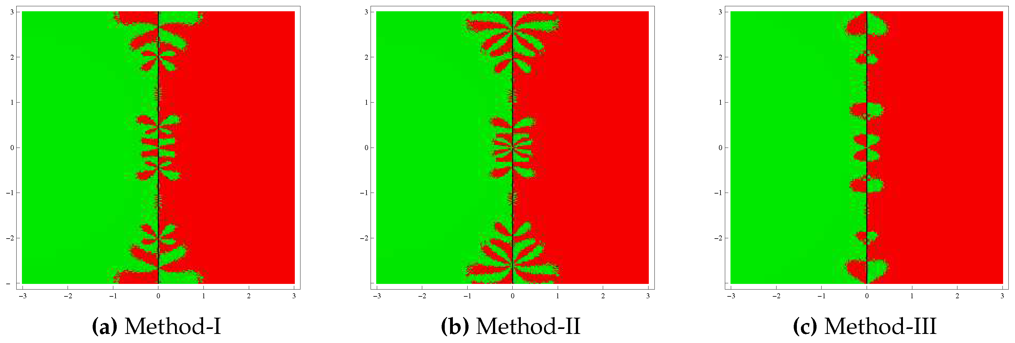
In our experiments, we took a square region $D=[-3,3]\times [-3,3]$ of the complex plane, with $400\times 400$ points, and applied the iterative methods starting with $z_0$ in the square. The numerical methods starting at point $z_0$ in a square can converge to the zero of the polynomial $P\left(z\right)$ or eventually diverge. The stopping criterion for convergence up to a maximum of 25 iterations was considered to be ${10}^{-3}$. If the desired tolerance was not achieved in 25 iterations, we did not continue and declared that the iteration from $z_0$ did not converge to any root. The strategy taken into account was this: a color was assigned to each starting point $z_0$ in the basin of a zero. Then, we distinguished the attraction basins by their colors. If the iterative function starting from the initial point $z_0$ converged, then it represented the basins of attraction with the particular assigned color, and if it diverged in 25 iterations, then it enters into the region of black color.

Test problem 1. Let $P_1\left(z\right)=z^2-1$ having the zeros $\{-1,1\}$. The basins of attractors generated by the methods for this polynomial are shown in Figure 1. From this figure, it can be observed that Method-III has more stable behavior than Methods I and II. In addition, Method-III exhibits very little chaotic behavior on the boundary points compared to other methods.

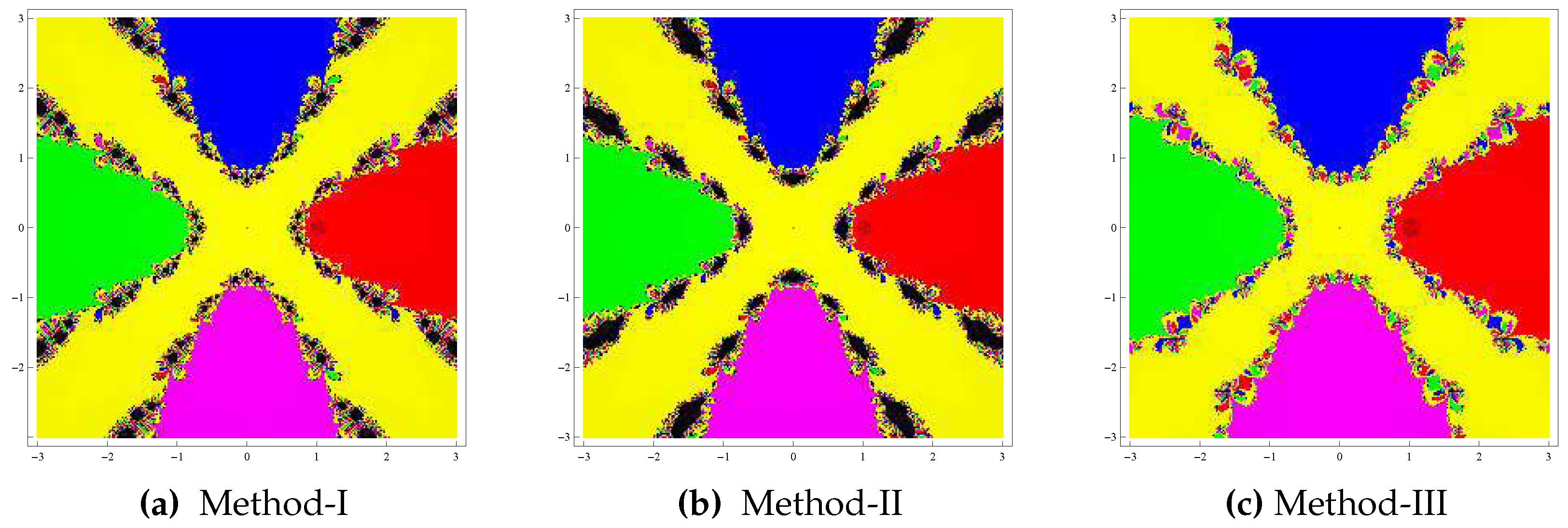
Test problem 2. Consider the polynomial $P_2\left(z\right)=z^3-1$ having the zeros $\{-\frac{1}{2}-\frac{\sqrt{3}}{2}i,-\frac{1}{2}+\frac{\sqrt{3}}{2}i,1\}$. The basins assessed by the methods are shown in Figure 2. In this case also, the Method-III has the largest basins of attraction compared to Methods I and II. On the other hand, the fractal picture of the Method-II has a large number of diverging points shown by black zones.

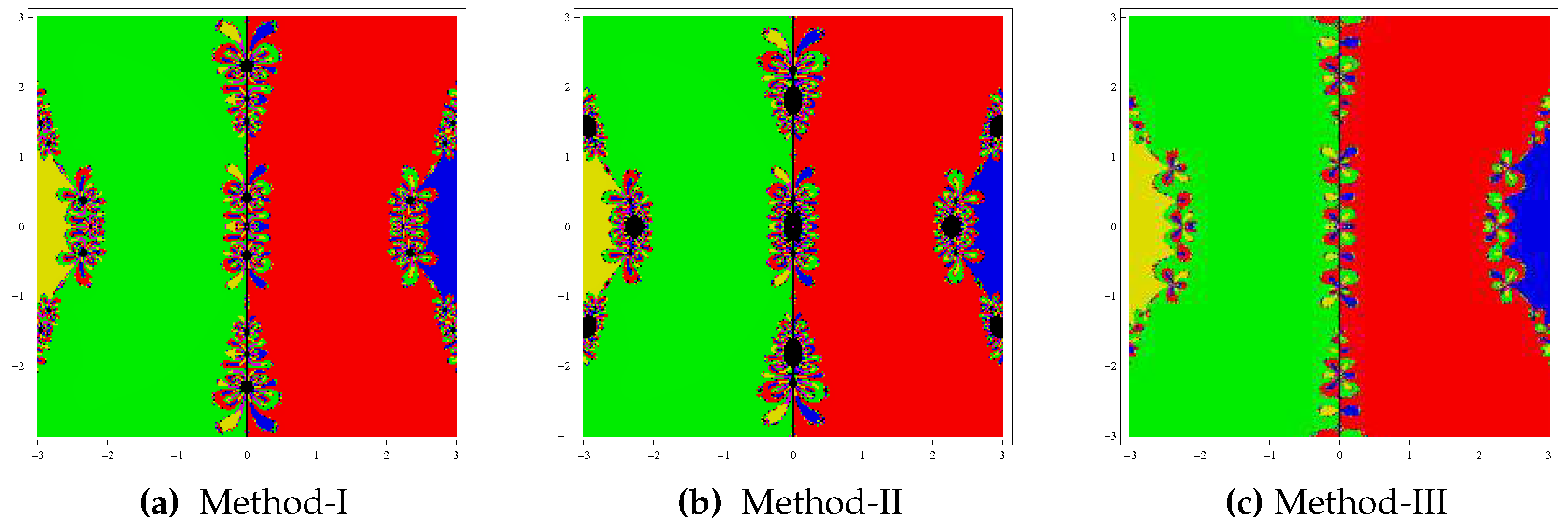
Test problem 3. Consider biquadratic polynomial $P_3\left(z\right)=z^4-10z^2+9$ having simple zeros $\{-3,-1,1,3\}$. The basins for this polynomial are exhibited in Figure 3. We observed that Method-III showed good convergence with wider basins of attraction of the zeros in comparison to other methods. We also noticed that Method-II had bad stability properties.

Test problem 4. Let $P_4\left(z\right)=z^5-z$ having simple zeros $\{-1,1,0,-i,i\}$. Like previous problems, in this problem also, Method-III had a good convergence property for the solutions in comparison to other methods (see Figure 4). Moreover, this was the best method in terms of the least chaotic behavior on the boundary points. On the contrary, Method-II had the highest number of divergent points, and was followed by Method-I.

5. Conclusions

In the present study, we discussed the convergence of existing Jarratt-like methods of sixth order. In the earlier study of convergence, the conditions used were based on Taylor’s expansions requiring up to the sixth or higher-order derivatives of function, although the iterative procedures used first-order derivatives only. It is quite well understood that these hypotheses restrict the applications of the scheme. However, the present study extended the suitability of methods by using assumptions on the first-order derivative only. Moreover, this approach provides the radius of convergence, bounds on error, and estimates on the uniqueness of the solution of equations. These important elements of convergence are not established by the approaches such as Taylor series expansions with higher order derivatives which may not exist, may be costly, or may be difficult to calculate. So, we do not have any idea how close the initial guess was to the solution of convergence for the method. That is to say the initial guess is a shot in the dark by the approaches of applying Taylor series expansions. Theoretical results of convergence so obtained are verified by numerical testing. Finally, the convergence regions of the methods were also assessed by a graphical drawing tool; namely, basin of attraction.

References

1. Rheinbolt, W.C. An adaptive continuation process for solving system of nonlinear equations. In Mathematical Models and Numerical Methods; Banach Center: Warsaw Poland, 1977; pp. 129–142. [Google Scholar]
2. Argyros, I.K. Computational Theory of Iterative Methods; Series: Studies in Computational Mathematics; Chui, C.K., Wuytack, L., Eds.; Elsevier Publ. Co.: New York, NY, USA, 2007; Volume 15. [Google Scholar]
3. Argyros, I.K.; Magreñán, Á.A. Iterative Methods and Their Dynamics with Applications; CRC Press: New York, NY, USA, 2017. [Google Scholar]
4. Argyros, I.K.; Sharma, J.R.; Kumar, D. Ball convergence of the Newton–Gauss method in Banach space. SeMA J. 2017, 74, 429–439. [Google Scholar] [CrossRef]
5. Babajee, D.K.R.; Dauhoo, M.Z.; Darvishi, M.T.; Barati, A. A note on local convergence of iterative methods based on Adomian decomposition method and 3-note quadrature rule. Appl. Math. Comput. 2008, 200, 452–458. [Google Scholar] [CrossRef]
6. Argyros, I.K.; Kumar, D.; Sharma, J.R. Study of optimal eighth order weighted-Newton methods in Banach spaces. Commun. Korean Math. Soc. 2018, 33, 677–693. [Google Scholar]
7. Argyros, I.K.; Sharma, J.R.; Kumar, D. On the local convergence of weighted-Newton methods under weak conditions in Banach spaces. Ann. Univ. Sci. Budapest. Sect. Comp. 2018, 47, 127–139. [Google Scholar]
8. Kumar, D.; Argyros, I.K.; Sharma, J.R. Convergence ball and complex geometry of an iteration function of higher order. Mathematics 2019, 7, 28. [Google Scholar] [CrossRef] [Green Version]
9. Sharma, J.R.; Kumar, D. A fast and efficient composite Newton–Chebyshev method for systems of nonlinear equations. J. Complex. 2018, 49, 56–73. [Google Scholar] [CrossRef]
10. Sharma, J.R.; Argyros, I.K.; Kumar, D. Newton-like methods with increasing order of convergence and their convergence analysis in Banach space. SeMA J. 2018. [Google Scholar] [CrossRef]
11. Hernández, M.A.; Salanova, M.A. Modification of Kantrovich assumptions for semilocal convergence of Chebyshev method. J. Comput. Appl. Math. 2000, 126, 131–143. [Google Scholar] [CrossRef] [Green Version]
12. Gutiérrez, J.M.; Magreñán, A.A.; Romero, N. On the semilocal convergence of Newton-Kantrovich method under center-Lipschitz conditions. Appl. Math. Comput. 2013, 221, 79–88. [Google Scholar]
13. Jaiswal, J.P. Semilocal convergence of an eighth-order method in Banach spaces and its computational efficiency. Numer. Algor. 2016, 71, 933–951. [Google Scholar] [CrossRef]
14. Jaiswal, J.P.; Pandey, B. Recurrence relations and semilocal convergence of a fifth order method in Banach spaces. Int. J. Pure Appl. Math. 2016, 108, 767–780. [Google Scholar] [CrossRef] [Green Version]
15. Darvishi, M.T.; Barati, A. A third-order Newton-type method to solve systems of nonlinear equations. Appl. Math. Comput. 2007, 187, 630–635. [Google Scholar] [CrossRef]
16. Darvishi, M.T.; Barati, A. A fourth-order method from quadrature formulae to solve systems of nonlinear equations. Appl. Math. Comput. 2007, 188, 257–261. [Google Scholar] [CrossRef]
17. Xiao, X.; Yin, H. A simple and efficient method with high order convergence for solving systems of nonlinear equations. Comput. Math. Appl. 2015, 69, 1220–1231. [Google Scholar] [CrossRef]
18. Narang, M.; Bhatia, S.; Kanwar, V. New two-parameter Chebyshev–Halley–like family of fourth and sixth–order methods for systems of nonlinear equations. Appl. Math. Comput. 2016, 275, 394–403. [Google Scholar] [CrossRef]
19. Xiao, X.; Yin, H. Achieving higher order of convergence for solving systems of nonlinear equations. Appl. Math. Comput. 2017, 311, 251–261. [Google Scholar] [CrossRef]
20. Jarratt, P. Some effcient fourth order multipoint methods for solving equations. BIT 1969, 9, 119–124. [Google Scholar] [CrossRef]
21. Jarratt, P. Some fourth order multipoint iterative methods for solving equations. Math. Comput. 1966, 20, 434–437. [Google Scholar] [CrossRef]
22. Jarratt, P. Multipoint iterative methods for solving certain equations. Comput. J. 1966, 8, 398–400. [Google Scholar] [CrossRef] [Green Version]
23. Alzahrani, A.K.H.; Behl, R.; Alshomrani, A. Some higher-order iteration functions for solving nonlinear models. Appl. Math. Comput. 2018, 334, 80–93. [Google Scholar] [CrossRef]
24. Cordero, A.; Hueso, J.L.; Martínez, E.; Torregrosa, J.R. A modified Newton–Jarratt’s composition. Numer. Algor. 2010, 55, 87–99. [Google Scholar] [CrossRef]
25. Sharma, J.R.; Arora, H. Efficient Jarratt–like methods for solving systems of nonlinear equations. Calcolo 2014, 51, 193–210. [Google Scholar] [CrossRef]
26. Sharma, J.R.; Kumar, D.; Argyros, I.K.; Magreñán, Á.A. On a bi–parametric family of fourth order composite Newton–Jarratt methods for nonlinear systems. Mathematics 2019, 7, 492. [Google Scholar] [CrossRef] [Green Version]
27. Ahmad, F.; Tohidi, E.; Ullah, M.Z.; Carrasco, J.A. Higher order multi–step Jarratt–like method for solving systems of nonlinear equations: Application to PDEs and ODEs. Comp. Math. Appl. 2015, 70, 624–636. [Google Scholar] [CrossRef] [Green Version]
28. Junjua, M.U.D.; Akram, S.; Yasmin, N.; Zafar, F. A new Jarratt–type fourth-order method for solving system of nonlinear equations and applications. J. Appl. Math. 2015, 14. [Google Scholar] [CrossRef]
29. Weerakoon, S.; Fernando, T.G.I. A variant of Newton’s method with accelerated third-order convergence. Appl. Math. Lett. 2000, 13, 87–93. [Google Scholar] [CrossRef]
30. Burden, R.L.; Faires, J.D. Numerical Analysis; Brooks/Cole: Boston, MA, USA, 2005. [Google Scholar]
Figure 1. Basins of attraction for test problem 1.
Mathematics 07 01203 g001
Figure 2. Basins of attraction for test problem 2.
Mathematics 07 01203 g002
Figure 3. Basins of attraction for test problem 3.
Mathematics 07 01203 g003
Figure 4. Basins of attraction for test problem 4.
Mathematics 07 01203 g004