Article

Comparative Analysis of Machine Learning Models for Prediction of Remaining Service Life of Flexible Pavement

by
Narjes Nabipour
1,
Nader Karballaeezadeh
2,
Adrienn Dineva
3,
Amir Mosavi
3,4,
Danial Mohammadzadeh S.
5,6 and
Shahaboddin Shamshirband
7,8,*
1
Institute of Research and Development, Duy Tan University, Da Nang 550000, Vietnam
2
Department of Civil Engineering, Shahrood University of Technology, Shahrood 3619995161, Iran
3
Institute of Automation, Kalman Kando Faculty of Electrical Engineering, Obuda University, 1034 Budapest, Hungary
4
Queensland University of Technology, 130 Victoria Park Road, Queensland 4059, Australia
5
Department of Civil Engineering, Ferdowsi University of Mashhad, Mashhad 9177948974, Iran
6
Department of Elite Relations with Industries, Khorasan Construction Engineering Organization, Mashhad 9185816744, Iran
7
Department for Management of Science and Technology Development, Ton Duc Thang University, Ho Chi Minh City, Vietnam
8
Faculty of Information Technology, Ton Duc Thang University, Ho Chi Minh City, Vietnam
*
Author to whom correspondence should be addressed.
Mathematics 2019, 7(12), 1198; https://doi.org/10.3390/math7121198
Submission received: 19 October 2019 / Revised: 30 November 2019 / Accepted: 2 December 2019 / Published: 6 December 2019

Abstract

:
Prediction of the remaining service life (RSL) of pavement is a challenging task for road maintenance and transportation engineering. The prediction of the RSL estimates the time that a major repair or reconstruction becomes essential. The conventional approach to predict RSL involves using non-destructive tests. These tests, in addition to being costly, interfere with traffic flow and compromise operational safety. In this paper, surface distresses of pavement are used to estimate the RSL to address the aforementioned challenges. To implement the proposed theory, 105 flexible pavement segments are considered. For each pavement segment, the type, severity, and extent of surface damage and the pavement condition index (PCI) were determined. The pavement RSL was then estimated using non-destructive tests include falling weight deflectometer (FWD) and ground-penetrating radar (GPR). After completing the dataset, the modeling was conducted to predict RSL using three techniques include support vector regression (SVR), support vector regression optimized by the fruit fly optimization algorithm (SVR-FOA), and gene expression programming (GEP). All three techniques estimated the RSL of the pavement by selecting the PCI as input. The correlation coefficient (CC), Nash–Sutcliffe efficiency (NSE), scattered index (SI), and Willmott’s index of agreement (WI) criteria were used to examine the performance of the three techniques adopted in this study. In the end, it was found that GEP with values of 0.874, 0.598, 0.601, and 0.807 for CC, SI, NSE, and WI criteria, respectively, had the highest accuracy in predicting the RSL of pavement.

1. Introduction

Pavement performance prediction models are an essential part of pavement management systems (PMSs) [1,2,3,4]. In addition to estimating the future condition of the pavement, these models help pavement engineers in the following [5,6]: (1) determining the optimal time for maintenance, rehabilitation, and reconstruction (MR&R) activities, (2) suggesting the most economical MR&R strategies, (3) estimating the required budget for MR&R activities, and (4) anticipating the results of various strategies. Until the late 1950s, little attention was paid to pavement performance and pavements were often categorized as satisfactory or unsatisfactory [7]. With the development of computational methods and the presentation of ML methods, many researchers have studied and developed pavement performance prediction models. These models differ in two respects: firstly, the index that was adopted as a criterion for pavement performance, secondly, the selected approach for modeling.
Through reviewing the pavement performance models, it was found that the Pavement Condition Index (PCI) [8], International Roughness Index (IRI) [3,9,10,11,12], Present Serviceability Index (PSI) [5,13], Remaining Service Life (RSL) [14], and Present Serviceability Ratio (PSR) [15] indices were more commonly used by the researchers. In terms of the modelling approach, methods such as artificial neural networks (ANN) [5,12], support vector machine (SVM) [1,11,14,15], radial basis function (RBF) [11], gene expression programming (GEP) [10], regression tree (RT) [13,16], Random Forest (RF) [3,17], and genetic programming (GP) [8] were used in the literature.
In general, pavement management activities are split into two categories [18]: network-level management and project-level management. Project-level management specifies roads that need to be repaired, repair process, and repair timetable. Therefore, predicting future conditions of pavement is essential for project management [18]. Forecasting pavement future conditions will require ongoing pavement assessment and inspection that will improve the operational quality of maintenance operations [19,20]. On the other hand, network-level management focuses on determining the budget required to preserve the pavement network at the standard level. Hence, it is indispensable to determine the RSL of pavement at this level of management [18]. Various factors such as traffic, characteristics of pavement materials, subgrade properties, climatic conditions, and maintenance quality have a destructive impact on the road pavement. As a result, pavement service life is surrounded by uncertainties that complicate the prediction of RSL [21].
The necessity of determining RSL in the previous paragraph has been recognized. Besides RSL, the other common indicators of pavement performance is PCI, which represents the general conditions of the pavement surface and ranges from zero for a practically unusable pavement to 100 for a flawless pavement (according to ASTM D-6433-07) [22]. PCI is determined based on pavement inspection results in terms of type, severity, and the extent of distresses [23,24]. After a thorough inspection of pavement surface distresses by an experienced inspector, PCI will be determined according to the related standard [22]. PCI is an index adopted in the project-level pavement management process. Hence, this index is specified before entering network-level pavement management. Conversely, the RSL of pavement, which is one of the pillars of network-level pavement management, is determined by applying the falling weight deflectometer (FWD) non-destructive test. In this test, a traffic lane is first blocked. Then an impulsive loading is applied to the pavement to induce pavement surface deflections. By analyzing pavement surface deflections, the RSL is calculated. In addition to the characteristics of the pavement layers materials (Young’s modulus and Poisson’s ratio) required for back-analysis in stress and strain calculations, a key point in calculating the RSL using the above method is knowing the pavement layers thickness for the analysis of deflections. The thickness of the pavement layers is determined using the ground-penetrating radar (GPR) non-destructive test. As a result, two non-destructive tests are required to determine the RSL of pavement. Traffic interference during FWD and GPR tests should also not be forgotten.
In light of the above, the current method of determining RSL is not only costly but also compromises the safety of users due to traffic interference during testing. Given the limited budget resources of transportation agencies, determining the RSL of pavement to manage a pavement network represents one of the ongoing concerns of such agencies [20]. Considering the necessity of RSL determination for PMSs as well as the problems mentioned in the current procedure of RSL determination, a new pavement performance model is proposed in this paper. In this study, three methods of SVR, SVR-FOA (support vector regression optimized by the fruit fly optimization algorithm), and GEP have been applied to predict the RSL of road pavements. Given the importance and widespread use of PCI in PMSs, RSL modeling was based on PCI.
The main objective of this study was to save time, reduce costs, and increase safety in the RSL determination process. According to the PCI calculation on project-level activities, using PCI for network-level management operations, estimation of RSL, will contribute to the overlapping of activities and saving time. The methods presented in this paper, by excluding non-destructive tests from the process of determining the RSL of pavement, drastically reduce costs. On the other hand, by eliminating non-destructive tests, traffic interference during testing and the potential safety hazards to road users are also eliminated.
The data required for developing the innovative SVR-FOA method proposed in this paper was collected from Shahrood–Damghan highway in the Semnan province, Iran. The pavement type of this highway is flexible. In this highway, a 100-m long pavement segment was taken from the beginning of each kilometer, and after assessing the surface distresses of each segment, its PCI was calculated. In the next step, FWD and GPR tests were applied to the selected segments to determine the RSL. Finally, using three SVR, SVR-FOA, and GEP methods, the RSL modeling based on PCI was implemented.
This paper is organized as follows: Section 2 offers a review of studies on the prediction of RSL. Section 3 introduces the method employed in this study. This section is made of four sub-sections titled PCI, RSL, machine learning techniques, and case study. In Section 4, the results of the analyses are presented and discussed. Finally, the conclusions are drawn in Section 5.

2. Literature Review

PMS is an Assessment Management System (AMS) used by road network administrators to maintain the entire network at the desired level. Predicting pavement performance is a key factor in PMSs [25]. The models of predicting pavement’s RSL fall into the category of the pavement performance prediction models. In this section, studies carried out by other researchers on predicting RSL are reviewed. Table 1 lists the results of studies that have strived to estimate RSL to date.
In Table 1, the models of determining the RSL of pavement are divided into three categories based on the model inputs:
  • First category: Models that predict the RSL based on the response (stress and strain) of pavement to the applied loads.
  • Second category: Models that predict the RSL based on pavement quality indices.
  • Third category: Models that predict the RSL based on the results of pavement non-destructive tests.
Among the above categories, models that predict the remaining pavement service based on qualitative indices appear to be more appropriate. It is because such models neither call for the analysis of pavement behavior and response, as in the first category nor require non-destructive tests, like the third category. Instead, they estimate the RSL of the pavement by assessing pavement and calculating a qualitative index in the simplest possible way. In light of the above points, in this paper, PCI has been adopted as a qualitative index for predicting RSL. Setyawan et al. conducted a similar study on East Line of South Sumatera the results of which are displayed in Table 1. They evaluated the condition of road performance and damages and determined PCI. Then they calculated the RSL of the pavement using the deflection data acquired from falling weight deflectometer measurements. Finally, the relationship between these two values was examined. The research involves five sections of the route with the different damaged condition. After calculating the PCI and RSL values, the relationship between these two parameters was determined with the help of Microsoft Excel software The model presented in their study has two drawbacks: (1) The number of data for building a reliable model is too small, (2) instead of using simple regression with Microsoft Excel, more advanced methods, such as ML can be used to achieve better results. In contrast, the methods proposed in this paper are based on the data gathered from 105 pavement segments using machine learning methods.
In general, PCI offers a valid index accepted by all transportation agencies around the world, and it is widely used in their evaluations. Compared to the current method of estimating the RSL of pavements (using two non-destructive FWD and GPR tests), the proposed method provides a far simpler, safer, and less costly way of estimating RSL.

3. Methodology

3.1. Pavement Condition Index (PCI)

Extensively used in roads, parking lots, and airports, PCI is recognized as a standard practice by many organizations around the world, including the Federal Aviation Administration, the American Public Works Association, and the U.S. Air Force [34]. PCI is a numerical index that expresses the rate of pavement surface distresses. PCI exhibits structural integrity and Surface operational condition but is not able to measure structural capacity [22].
The first step in determining the PCI of each pavement segment is to determine the type, extent, and severity of surface distresses. The second step is to determine the deduct values (DVs) with the help of the specific curves for each type of distress. Next, reduce the number of DVs to the maximum number allowed (mi) [22,34]:
m i = 1 + ( 100 HDV ) × 9 98   ,
where HDV = greatest individual deduct value.
Next, specify the number of DVs greater than 2 (q). In the next step, the corrected deduct value (CDV) should be specified in a special curve with the help of TDV (sum of DVs) and q [34]. Then among DVs that are larger than 2, decrease the smallest ones to 2. At this point, repeat the process of calculating q, computing CDV, and reducing DV until q is equal to 1. By calculating the maximum CDV, PCI can be calculated [22,34]:
PCI = 100 C D V m a x
Readers can refer to [22] and [34] for reaching more details and related curves. The classification of a pavement segment based on PCI follows Table 2.

3.2. Remaining Service Life (RSL)

The RSL of pavement under operation is a key factor in implementing PMSs. It is because learning about the future conditions of the pavement network is essential for decision making, life cycle cost analysis, planning, and budget allocation [14,35]. In general, the definitions of RSL by different agencies and departments of transportation can be split into two general categories [36]:
  • The remaining time to reach a level of distress when the pavement needs to be rehabilitated or reconstructed. For example, the Minnesota Department of Transportation (MnDOT) defines the RSL as the time until the next major rehabilitation.
  • The time until pavement conditions reach a specific condition index limit. For example, the Michigan Department of Transportation (MDOT) defines the RSL based on the Michigan Ride Quality Index, assuming an RSL of zero when the said index is 50.
The RSL of pavement segments in this paper has been determined using the heavy falling weight deflectometer (HWD). The HWD is an FWD, the application of which is not constricted to the road and could be used for airport pavement assessment. Figure 1 shows the HWD device employed in this study.
The HWD applies a tension similar to the standard axle load (8.2 t) to the pavement surface over 10 to 35 ms. A number of geophones are placed on the pavement surface at specified distances from the loading center. The task of the geophones is to record the pavement deflections induced by the load applied with the HWD device. Standard axle load simulation in HWD is generated by a series of weight drops on a loading plate placed on the pavement surface [14]. Table 3 reveals the details of the HWD test undertaken in this study.
The deflections recorded by geophones are transferred to the central computer in HWD. In this computer, the analysis of pavement surface deflections is performed using ELMOD6 software. ELMOD uses Miner’s Law to calculate critical stresses and strains. Miner’s Law is used to interact with the impact of distresses that occur during each season and by each load. With the help of back-calculation analysis, ELMOD provides important outputs including RSL, overlay thickness, and elasticity module [38].
A prerequisite of estimating RSL in accordance with the process described in this section is knowing the thickness of pavement layers. For determining the pavement layer’s thickness, GPR non-destructive testing was carried out for all pavement segments. GPR is capable of calculating pavement thickness as a continuous profile by transmitting electromagnetic waves through a transmit antenna and receiving recursive signals [39]. The receiver of GPR takes reflected waves and shows them as a plot of amplitude and time [40]. The layers thickness (hi) of the pavement is calculated by the following equation [41]:
h i = c Δ t i ε r   ,
where Δ t i = time between amplitudes Ai and Ai+1, c = electromagnetic wave speed through the vacuum, and ε r = the relative dielectric constant of the layer. Table 4 shows the complete details of the GPR experiment carried out in this study.

3.3. Machine Learning Techniques

In this paper, the main objective is to present a new approach for predicting the RSL of flexible pavements based on PCI using machine learning techniques. The data set consisted of the RSL and PCI of all segments under study, which were analyzed using the GEP, SVR, and SVR-FOA methods. GEP is an evolutionary algorithm that investigates the relationship between input and output variables by developing computer programs [44]. Different from both the genetic algorithm (GA) and genetic programming (GP), GEP is a combination of both introduced by Ferreira in 2001 [45]. SVR is a supervised machine learning technique employed to solve regression problems. SVR is especially popular due to its desirable management and performance in handling nonlinear issues [46]. The success of an SVR in problem-solving depends on the proper selecting of its basic parameters. SVR’s basic parameters include c, ε, and kernel function parameters [14]. Improper values of the basic parameters in the SVR can lead to under-fitting or over-fitting. Thus, the optimum values of them must be selected during training the SVR method [47]. In other words, different optimization algorithms were developed and may be utilized for selecting the suitable values of SVR. FOA is an intelligent swarm algorithm introduced by Pan in 2012, which utilizes the food searching strategy of a fruit fly to find the optimal values for SVR basic parameters [48]. These methods are introduced in the following subsections.

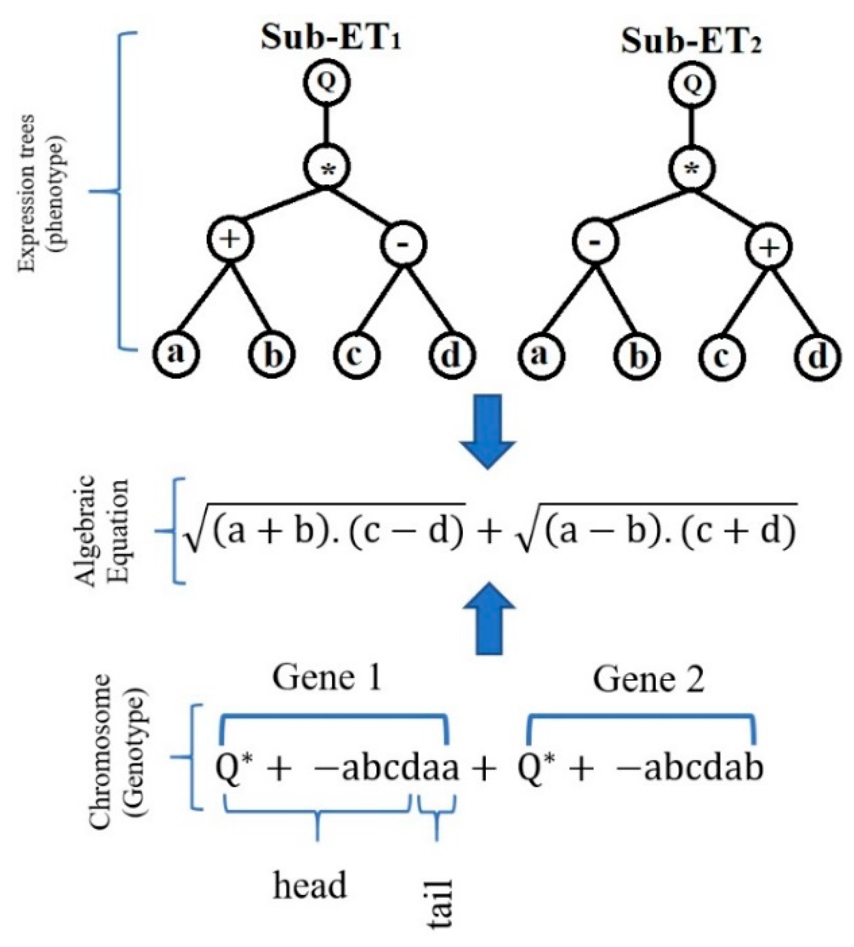
3.3.1. Gene Expression Programming (GEP)

GEP is a developed GP method that solves a problem by creating expression trees (ETs). In fact, GEP is an evolutionary algorithm for creating computer programs. The designed computer programs have sophisticated tree structures that are trained similar to a living organism by changing size, shape, and composition, and adapted to the conditions. Like living organisms, GEP programs are coded as simple fixed-length linear chromosomes. Hence, GEP is a genotype-phenotype system that employs a simple genome to store and transmit genetic information and adopts a complex phenotype to explore and adapt to the environment. The genome consists of a chromosome or a fixed-length string that combines one or more genes of the same size. In fact, each chromosome contains one or more genes known as Sub-ETs. In GEP, all Sub-ETs are linked through the root with connection functions. The connection functions in GEP include division, multiplication, subtraction, and addition [49]. Figure 2 shows an instance of the genotype-phenotype structure in GEP.
These genes, despite their fixed length, are coded for ETs of varying size and shape. It implies that the size of the coding region varies from one gene to another to allow for progressive adaptation and evolution. Each gene has a coding area called open reading frame (ORF), which, after being coded as an expression tree, provides a solution to the problem [51]. Figure 3 demonstrates the coding region (ORF), the non-coding region, and the expression tree for a gene.
Like other evolutionary approaches, GEP begins by randomly generating the initial population chromosomes. In the first population, each chromosome is assessed based on the fitness function and receives a fitness value. Various fitness functions have been used in GEP, including root relative squared error (RRSE), relative square error (RSE), root mean square error (RMSE), and mean square error (MSE) [44]. The proper chromosomes are more likely to be picked in the next generation. After being selected, chromosomes are amended by genetic operators (including transposition, inversion, mutation, recombination, and gene crossover) and then reconstructed. This process is sustained until a suitable solution or the maximum number of generations is reached [44,53].

3.3.2. Support Vector Regression (SVR)

The SVR is considered as a support vector machine (SVM) used for regression problems. SVR has been widely used for civil engineering problems [54,55]. Supervised learning techniques, including SVR, utilize structural risk minimization (SRM), while conventional neural networks use empirical risk minimization (ERM). ERM minimizes the error of training samples, but SRM is able to minimize a higher level of error. As a result, SVM is capable of overcoming the deficiencies of conventional neural networks [14,46]. The main idea in SVR is to map nonlinear information into a higher dimensional space and then solve a linear regression problem in the new space [46,56,57]. In the new space, a simple linear kernel function is adopted to solve the problem. However, in complex problems, a simple linear kernel function will be inadequate. The kernel function k(x, z) for all x ,   z X is defined as follows [46]:
k ( x , z ) = φ ( x ) · φ ( z ) .
Each kernel function must have two features [46]:
1. Symmetricity
k ( x , z ) = φ ( x ) · φ ( z ) = φ ( z ) · φ ( x ) = k ( z , x ) ,
2. Compliance with the Cauchy-Schwartz criterion
k ( x , z ) 2 = φ ( x ) · φ ( z ) 2     φ ( x ) 2 φ ( z ) 2 .
These two conditions guarantee that the new space is definable by the kernel function. The most famed kernel functions are polynomial kernel, radial basis functional kernel, linear kernel, and sigmoid kernel [57]. Given the above explanation, it is clear that SVR requires an appropriate function to explain the nonlinear relationship between input (xi) and output (yi) [57]:
f ( x i ) = w · φ ( x i ) + b ,
where φ ( x i ) = transformation function, w = weight, b = bias. w and b are obtained by minimizing the following function, which is known as the regularized risk function [57]:
R ( w ) = 1 2 w 2 + C i = 1 N L ε ( y i , f ( x i ) ) ,
where 1 2 w 2 = regularization term, C = penalty coefficient, and L ε ( y i , f ( x i ) ) = ε -insensitive loss function:
L ε ( y i , f ( x i ) ) = max { 0 ,   | y i f ( x i ) | ε } ,
where ε = permitted error threshold.
To solve the optimization boundaries, two factors of ξ and ξ are defined [57]:
m i n f ( w ,   ξ ,   ξ ) = 1 2 w 2 + C i = 1 N ( ξ ,   ξ ) ,
subject to
{ y i [ w · φ ( x i ) ] b ε + ξ , ξ 0 [ w · φ ( x i ) ] + b y i ε + ξ , ξ 0   .
We now need to define a Lagrange function based on the objective function and boundary conditions [57]:
m a x H ( i ,   i + ) = 1 2 i = 1 N j = 1 N ( i i + ) ( j j + ) K ( x i   ,   x j ) +   i = 1 N y i ( i   i + )   ε i = 1 N y i ( i +   i + ) ,
subjected to
i = 1 N y i ( i   i + ) = 0 , i ,   i +   [ 0   , C ] .
Therefore, the regression function can be shown as follows [57]:
f ( x ) = i = 1 N ( i i + ) K ( x i   ,   x j ) + b ,
where K ( x i   ,   x j ) = kernel function. Figure 4 summarizes the overall structure of the SVR.
In general, SVR performance depends on its parameters. SVR parameters are [59,60]:
  • ε : this parameter supervises the width of the ε -insensitive zone, used to fit the training data. The value ε can affect the number of support vectors used to build the regression function. For the bigger ε , estimates are more ‘flat’, and the fewer support vectors are chosen.
  • C: this parameter specifies the trade-off between the complexity of the model and the grade to which deviations larger than ε are bearable in optimization formulation.
  • γ : this parameter determines the relation between error minimization and smoothness of the estimated function.
These parameters are chosen by the user based on prior knowledge of SVR, so this method is not suitable for non-professional users. Various algorithms have been developed to optimize the amounts of SVR parameters. In the following subsection, one of the optimization algorithms used in this paper is introduced.

3.3.3. Fruit Fly Optimization Algorithm (FOA)

FOA is an optimization algorithm developed based on the food search behavior of the Drosophila insect [48]. The fruit fly has superior smell and vision senses, which discriminates it from other insects. Fruit flies track the smell of the food sources dispersed through the air and heads towards it. This insect is even capable of smell tracking from a distance of 40 km. When approaching the food source, the fruit fly employs a sense of vision to locate food and other fruit flies. The best information is shared among the fruit flies, and finally, the route leading to the food source is identified [61]. Figure 5 illustrates the process of food search by a fruit fly.
In this paper, this optimization algorithm has been selected to find the optimal values of SVR parameters, which is known as SVR-FOA. The general steps of SVR-FOA can be summarized as follows [63,64]. The flowchart of the SVR-FOA method is illustrated in Figure 6.
Step 1. SVR parameters ( ε , c) initialization and kernel function determination.
Step 2. Parameter initialization; including the maximum number of iterations, location of initial population (X-axis, Y-axis), population size, and random flight distance domain:
X _ a x i s = r a n d s ( 1 , 2 ) ,
Y _ a x i s = r a n d s ( 1 , 2 ) .
Step 3. Population initialization
A random location (Xi, Yi) and food founding distance are assigned to each fruit fly:
X i = X _ a x i s + R a n d o m   v a l u e ,
Y i = Y a x i s + + R a n d o m   v a l u e ,
where: i = Population size.
Step 4. Population evaluation
The distance from the origin to the food source (D) and the smell concentration parameter (S) are calculated:
D i = X i 2 + Y i 2 ,
S i = 1 D i .
Step 5. Replacement
S value is substituted with the fitness function or smell concentration judgment function so that the smell concentration for each fruit fly location can be attained:
S m e l l i = F u n c t i o n   ( S i ) .
Step 6. Detect the maximal smell concentration
At this point, the fruit fly with the highest Si is identified and located within the population.
[ b e s t S m e l l b e s t I n d e x ] = max ( S m e l l ) .
Step 7. Keep smell concentration
The coordinates of the maximum smell concentration are set, and the fruit fly swarm flows in that direction,
X _ a x i s = X ( b e s t I n d e x ) ,
Y _ a x i s = Y ( b e s t I n d e x ) .
Step 8. Iterative optimization
Steps 3 to 6 are repeated until the smell concentration does not show any improvement compared to the previous one or the maximum number of repetitions in Step 2 is reached.
Step 9. Output the optimum parameter of SVR.

3.4. Case Study

To implement the theory proposed in this paper, a stretch of 105 km from Shahrood–Damghan highway in Iran was selected and inspected. Given that this highway is part of the route between Tehran (the capital of Iran) and Mashhad (the second most important city of Iran), it constitutes one of the major roads. The highway consists of two lanes in each direction and uses the flexible pavement. A prerequisite of implementing the proposed theory is to select a number of sample segments from his highway. To do so, segments 100 m in length and 7 m in width were selected from the beginning of each kilometer. By inspecting the selected segments, the surface distress data (type, severity, and extent) of each segment was recorded in the assessment forms. The PCI of each segment was calculated as described in Section 3.1. With PCI known, the RSL of the pavement segments need to be known. Hence, HWD and GPR tests were performed on all segments and the RSL of each segment was determined. Figure 7 shows the location of the Shahrood–Damghan Highway as well as the starting and ending points of the segments understudy on this Google map.

4. Results and Discussion

The results of the analysis are presented in this subsection. First, the statistical specifications of the input and output modeling variables are listed in Table 5. The data was extracted from IBM SPSS 23 software (version 2015, International Business Machines Corporation (IBM), Armonk, New York, U.S.).
As depicted in Table 5, the mean PCI of all pavement segments is 59.97, which according to Table 2, is indicative of the fair state of all segments. The mean RSL of pavement is 17.77 years. For interpreting the mean RSL, it is worth noting that ELMOD6 software does not suggest the application of an overlay layer for this RSL. Hence, the average RSL of the segments is fairly desirable. Before calculating the correlation coefficient of the modeling input and output, the normality of the data must be determined. This is determined by kurtosis and skewness coefficients, as well as the results of the Kolmogorov–Smirnov test. In probability theory and statistics, kurtosis is a measure of the “tailedness” of the probability distribution of a real-valued random variable. Moreover, skewness is a measure of the asymmetry of the probability distribution of a real-valued random variable about its mean. The skewness value can be positive or negative, or undefined. A zero-skewness dataset has perfect symmetry (completely normal distribution). A positive/negative skew value indicates that the tail on the right/left side of the distribution is longer than the left/right side and the bulk of the values lie to the left/right of the mean. Kurtosis acts as a measure of the distribution peakedness. For a perfectly normal distribution, kurtosis should be zero. Positive kurtosis means a high peak distribution curve, and negative kurtosis refers to the flat-topped distribution curve [65,66]. It is very difficult to achieve zero skewness and Kurtosis, then the data distribution is normal when the skewness and Kurtosis values are between 2 and −2 [67]. So, it is clear from Table 5 that PCI, with lower kurtosis value, had better normal distribution than RSL. Kolmogorov–Smirnov is a non-parametric test that helps to determine if the data is normal or not. If the significance level (sig.) in this test is above 0.05, the data are normal [67]. When choosing a correlation test, even if one of the variables is abnormal, then the Spearman test is used. According to Table 5, since PCI variables have a normal distribution but RSL distribution is abnormal, the Spearman correlation test must be used. The correlation between PCI and RSL is 57.2%, which represents an average value.
As noted in Section 3.3.2, SVR consists of three basic parameters (C, ε, and γ), with the quality of SVR performance depending on the values selected for these three parameters. Table 6 shows the values of these basic parameters for the SVR as well as the optimized values of these parameters by the FOA algorithm.
In Table 7, the characteristics of the GEP model used in this study, including model parameters and genetic operators, are shown. It should be noted that the default parameters of Gene Expro Tools 4.0 software (Version 2.0, Gepsoft Limited, Bartolomeu Messines, Portugal) were selected for further computations.
Equation (25) shows the proposed formula of the GEP method, extracted from Gene Expro Tools 4.0, for estimating pavement remaining service life in terms of PCI:
RSL = 6.59964 + 322.568 PCI 8.96265 2.61881 PCI + PCI 1.18921 PCI 3 2 + 0.35035 ( 3.83258 PCI 9.83936 ) 9.83936 + PCI .
The results of scientific research are generally assessed with indicators that exhibit the accuracy and error of the analysis. In this study, four criteria entitled Correlation Coefficient (CC), Scattered Index (SI), Nash–Sutcliffe efficiency (NSE) and Willmott’s Index of agreement (WI) were used to determine the quality of the outputs [68,69]:
C C = i = 1 n R S L O i R S L p i 1 n i = 1 n R S L O i i = 1 n R S L p i ( i = 1 n R S L O i 2 1 n ( i = 1 n R S L O i ) 2 ) ( i = 1 n R S L p i 2 1 n ( i = 1 n R S L p i ) 2 ) ,
S I = 1 n i = 1 n ( R S L p i R S L O i ) 2 R S L O i ¯ ,
N S E = 1 i n ( R S L O i R S L p i ) 2 i n ( R S L O i R S L O i ¯ ) 2 ,
W I = 1 [ i = 1 n ( R S L p i R S L O i ) 2 i = 1 n ( | R S L p i R S L O i ¯ | + | R S L O i R S L O i ¯ | ) 2 ] ,
where RSLOi = observed RSL ith value, RSLPi = predicted RSL ith value, and RSL O i ¯ = average of RSLOi.
The CC is a number in the range of [−1, +1], with values of +1 and −1 indicating a complete correlation between model inputs and outputs. Positive values represent direct correlation and negative values demonstrate an inverse correlation. As the absolute value of CC approaches zero, the strength of the correlation decreases. SI represents an error and smaller values indicate lower errors in modeling. The highest NSE value is one with values close to one indicating greater modeling accuracy so that NSE = 1 represents the best modeling quality. WI is an index between 0 and 1 with values close to one suggesting higher modeling accuracy.
Table 8 reveals the four criteria introduced for all three methods employed in this study. To shed further light on the results of Table 8, a three-dimensional bar histogram of the criteria is presented in Figure 8. Based on the description in the preceding paragraph and the values in Table 8, it can be concluded that FOA has improved SVR results. Comparing the SVR-FOA and GEP modeling results, it can be contended that the GEP results are partially superior in the modeling proposed in this paper. Moreover, although the CC values of studied methods are not so high, due to lower SI values, they can be used with acceptable accuracy in RSL estimation.
There has been no standard method for splitting training and testing data. For instance, Choubin et al. [70] used a total of 63% of their data for model development, whereas Shamshirband et al. [71] utilized 67% of data, Mohammadzadeh et al. [72] 70%, and Samadarianfard et al. [73] implemented 80% of total data to develop their models. In this study, the dataset containing 105 pavement segments is used, where, approximately 70% of the data (i.e., 75 segments) are used for training, and the remaining 30 segments are utilized for testing. Figure 9 shows the RSL predicted by the three SVR, SVR-FOA, and GEP methods as well as the RSL measured in the HWD test for the segments selected as the test. As can be seen in Figure 9, the studied models do not accurately predict the maximum and minimum RSL values. So, this may affect the scheduling of maintenance actions.
Figure 10 displays the predicted RSL values versus the RSL values calculated by the HWD test for all three machine learning techniques adopted in this paper. In this regard, the method with the best prediction accuracy is the one that has a fit line equation of y = x, meaning that the line slope is equal to one and its intercept is equal to zero. Figure 10 is plotted for the test dataset. It can be comprehended from Figure 10, although the slope of trend lines of all studied methods is lower than 0.5, the accuracy of GEP is higher than SVR and SVR-FOA models.
Figure 11 represents the Taylor diagram used in this study. Introduced by Taylor in 2001, the Taylor diagram is a mathematical diagram that graphically allows a comparison of several models of a system. In this diagram, there are three categories of contours [74]:
  • Blue contours
    It shows the Pearson correlation coefficient.
  • Orange contours
    It indicates the RMS error that is proportional to the distance from a green spot on the horizontal axis called observed.
  • Black contours
    It indicates the standard deviation proportional to the radial distance from the center.
The presented Taylor Diagram shows the superior accuracy of the GEP model due to the lower distance of its correspondent point (the point with Magenta color) from the observed green point. Overall, by examining Figure 8, Figure 9, Figure 10 and Figure 11, it can be concluded that the SVR technique offers an average accuracy for the purpose of this article. Using the FOA algorithm to select the basic parameters of this technique significantly enhanced the accuracy of this method. On the other hand, the GEP method provides a formula for RSL prediction. By re-examining Figure 8, Figure 9, Figure 10 and Figure 11, it turned out that both SVR-FOA and GEP methods yielded desirable accuracy for RSL prediction. However, the accuracy of the GEP method was slightly higher than that of the SVR-FOA method.

5. Conclusions

Pavement management at both project and network levels are always associated with substantial costs. Due to the budget constraints inflicted on organizations in charge of PMS, optimizing pavement management costs is one of the priorities of any organization. RSL is a crucial factor for pavement management at the network level. The current procedure for determining RSL involves using FWD and GPR tests. These devices are not only costly but also interfere with the traffic flow and compromise the safety of road users. The aim subject of the study was to present a new approach for predicting the RSL of flexible pavement, which eliminated the drawbacks of current methods. Therefore, the proposed method can lead to lower costs, reduced time consumed, and also increase safety. The idea of estimating RSL has been followed by various researchers. The major differences between their studies were in the methodology and methods of analysis. After a review of previous studies on estimating the pavement RSL, we decided to use pavement surface distresses as a criterion for predicting RSL. Therefore, PCI pavement was employed as an input variable in modeling pavement RSL. Modeling was done with the help of ML techniques, which is the innovation of this research. The dataset utilized for modeling was selected from the Shahrood–Damghan highway in Iran. After selecting 105 pavement segments from the highway, PCI and RSL of all segments were determined. Modeling was conducted using GEP and SVR techniques after completing the dataset. The results of modeling with these techniques were evaluated based on four criteria include CC, SI, NSE, and WI, to determine the most appropriate technique for estimating pavement RSL. After exploring all four criteria, it was found that the GEP outcomes were far more accurate than the SVR. Then, to improve the accuracy of the SVR method, the FOA optimization algorithm was employed to add a third technique, as an innovative model (namely SVR-FOA), to the methods applied in this paper. Again, the four criteria CC, SI, NSE, and WI revealed a significant improvement in the accuracy of the SVR-FOA method compared to the SVR method, yet the GEP method still had the highest prediction precision. In sum, the findings of this paper suggested that the GEP method (with values of 0.874, 0.598, 0.601, and 0.807 for the four criteria CC, SI, NSE, and WI, respectively) offered an alternative to current methods of predicting pavement RSL. Based on the desired accuracy and the cost-benefit analysis, transportation agencies can use the GEP method to optimize the model accuracy, robustness, and reliability considering either new projects or for calibrating the former models.
In general, this study highlights the usefulness of the use of artificial intelligence in transportation engineering. The results show that artificial intelligence techniques can be used as an optimization tool (at time and cost) in pavement management systems. In terms of pavement engineering, this study concluded that the RSL of pavement, as a fundamental factor in the planning of the pavement network maintenance, is a flexible factor and is not limited to current cost-intensive methods. With the help of similar methods with the proposed method in this paper, the RSL can be determined as soon as possible. This will ease the future planning of road maintenance activities.

Author Contributions

Conceptualization, N.K.; methodology, N.K.; software, A.D., A.M., N.N., and S.S.; validation, A.D., A.M., N.N., and S.S.; formal analysis, A.K.; investigation, N.K., A.D., A.M., N.N., and S.S.; resources, X.X.; data curation, N.K., A.D., A.M., D.M.S., N.N., and S.S.; writing—original draft preparation, N.K.; writing—review and editing, A.M.; visualization, N.K.; supervision, S.S.; project administration, A.D. and A.M.; funding acquisition, A.D.

Funding

This work has been supported by the project GINOP-2.3.4-15-2016-00003.

Acknowledgments

This work has been supported by the project GINOP-2.3.4-15-2016-00003.

Conflicts of Interest

The authors declare no conflict of interest.

Acronyms

AbbreviationDescription
RSLRemaining Service Life
PCIPavement Condition Index
FWDFalling Weight Deflectometer
GPRGround Penetrating Radar
SVRSupport Vector Regression
SVR-FOASupport Vector Regression Optimized by Fruit Fly Optimization Algorithm
GEPGene Expression Programming
CCCorrelation Coefficient
NSENash–Sutcliffe Efficiency
SIScattered Index
WIWillmott’s Index of agreement
PMSsPavement Management Systems
MR&RMaintenance, Rehabilitation, and Reconstruction
IRIInternational Roughness Index
PSIPresent Serviceability Index
PSRPresent Serviceability Ratio
ANNArtificial Neural Network
SVMSupport Vector Machine
RBFRadial Basis Function
GEPGene Expression Programming
RTRegression Tree
RFRandom Forest
GPGenetic Programming
AMSAssessment Management System
DVDeduct Value
CDVCorrected Deduct Value
TDVSum of DVs
MnDOTMinnesota Department of Transportation
MDOTMichigan Department of Transportation
HWDHeavy Falling Weight Deflectometer
GAGenetic Algorithm
ETsExpression Trees
ORFOpen Reading Frame
RRSERoot Relative Squared Error
RSERelative Square Error
RMSERoot Mean Square Error
MSEMean Square Error
SVMSupport Vector Machine
SRMStructural Risk Minimization
ERMEmpirical Risk Minimization
FOAFruit Fly Optimization Algorithm

References

  1. Ziari, H.; Maghrebi, M.; Ayoubinejad, J.; Waller, S.T. Prediction of pavement performance: Application of support vector regression with different kernels. Transp. Res. Rec. 2016, 2589, 135–145. [Google Scholar] [CrossRef]
  2. Ismail, N.; Ismail, A.; Atiq, R. An overview of expert systems in pavement management. Eur. J. Sci. Res. 2009, 30, 99–111. [Google Scholar]
  3. Marcelino, P.; de Lurdes Antunes, M.; Fortunato, E.; Gomes, M.C. Machine learning approach for pavement performance prediction. Int. J. Pavement Eng. 2019, 12, 1–14. [Google Scholar] [CrossRef]
  4. Butt, A.A.; Shahin, M.Y.; Feighan, K.J.; Carpenter, S.H. Pavement Performance Prediction Model Using the Markov Process; Transportation Research Board: New York, NY, USA, 1987. [Google Scholar]
  5. Bianchini, A.P. Bandini, Prediction of pavement performance through neuro-fuzzy reasoning. Comput. Aided Civ. Infrastruct. Eng. 2010, 25, 39–54. [Google Scholar] [CrossRef]
  6. Broten, M. Local Agency Pavement Management Application Guide; Wiley: New York, NY, USA, 1997. [Google Scholar]
  7. Prozzi, J.A. Modeling Pavement Performance by Combining Field and Experimental Data; University of California: Oakland, CA, USA, 2001. [Google Scholar]
  8. Shahnazari, H.; Tutunchian, M.A.; Mashayekhi, M.; Amini, A.A. Application of soft computing for prediction of pavement condition index. J. Transp. Eng. 2012, 138, 1495–1506. [Google Scholar] [CrossRef]
  9. Ziari, H.; Sobhani, J.; Ayoubinejad, J.; Hartmann, T. Prediction of IRI in short and long terms for flexible pavements: ANN and GMDH methods. Int. J. Pavement Eng. 2016, 17, 776–788. [Google Scholar] [CrossRef] [Green Version]
  10. Mazari, M.D.D. Rodriguez, Prediction of pavement roughness using a hybrid gene expression programming-neural network technique. J. Traffic Transp. Eng. (Engl. Ed.) 2016, 3, 448–455. [Google Scholar] [CrossRef] [Green Version]
  11. Kargah-Ostadi, N.S.M. Stoffels, Framework for development and comprehensive comparison of empirical pavement performance models. J. Transp. Eng. 2015, 141, 04015012. [Google Scholar] [CrossRef]
  12. Kargah-Ostadi, N.; Stoffels, S.M.; Tabatabaee, N. Network-level pavement roughness prediction model for rehabilitation recommendations. Transp. Res. Rec. 2010, 2155, 124–133. [Google Scholar] [CrossRef]
  13. Terzi, S. Modeling the pavement present serviceability index of flexible highway pavements using data mining. J. Appl. Sci. 2006, 6, 193–197. [Google Scholar]
  14. Karballaeezadeh, N.; Mohammadzadeh, S.D.; Shamshirband, S.; Hajikhodaverdikhan, P.; Mosavi, A.; Chau, K.-W. Prediction of remaining service life of pavement using an optimized support vector machine (case study of Semnan–Firuzkuh road). Eng. Appl. Comput. Fluid Mech. 2019, 13, 188–198. [Google Scholar] [CrossRef]
  15. Ke-zhen, Y.; Liao, H.; Yin, H.; Huang, L. Predicting the pavement serviceability ratio of flexible pavement with support vector machines. In Road Pavement and Material Characterization, Modeling, and Maintenance; American Society of Civil Engineers: New York, NY, USA, 2011; pp. 24–32. [Google Scholar]
  16. Inkoom, S.; Sobanjo, J.; Barbu, A.; Niu, X. Prediction of the crack condition of highway pavements using machine learning models. Struct. Infrastruct. Eng. 2019, 15, 940–953. [Google Scholar] [CrossRef]
  17. Fathi, A.; Mazari, M.; Saghafi, M.; Hosseini, A.; Kumar, S. Parametric Study of Pavement Deterioration Using Machine Learning Algorithms. In Airfield and Highway Pavements 2019: Innovation and Sustainability in Highway and Airfield Pavement Technology; American Society of Civil Engineers Reston: Reston, VA, USA, 2019; pp. 31–41. [Google Scholar]
  18. Soncim, S.P.; de Oliveira, I.C.S.; Santos, F.B. Development of fuzzy models for asphalt pavement performance. Acta Sci. Technol. 2019, 41, e35626. [Google Scholar] [CrossRef]
  19. Arhin, S.A.; Williams, L.N.; Ribbiso, A.; Anderson, M.F. Predicting pavement condition index using international roughness index in a dense urban area. J. Civ. Eng. Res. 2015, 5, 10–17. [Google Scholar]
  20. Mfinanga, D.A. Sampling procedure for pavement condition evaluation of local collectors and access roads. Tanzan. J. Eng. Technol. 2007, 1, 99–109. [Google Scholar]
  21. Wahyudi, W.; Sandra, P.A.; Mulyono, A.T. Analysis of Pavement Condition Index (PCI) and Solution Alternative of Pavement Damage Handling Due to Freight Transportation Overloading (Case Study: National Road Section West Sumatra Border-Jambi City). In Proceedings of the Eastern Asia Society for Transportation Studies, Lalkatta, India, 2013. [Google Scholar]
  22. ASTM. ASTM D6433-07 Standard Practice for Roads and Parking Lots Pavement Condition Index Surveys; ASTM International: West Conshohocken, PA, USA, 2009. [Google Scholar]
  23. Marcelino, P.; Antunes, M.d.L.; Fortunato, E. Comprehensive performance indicators for road pavement condition assessment. Struct. Infrastruct. Eng. 2018, 14, 1433–1445. [Google Scholar] [CrossRef]
  24. Bryce, J.; Boadi, R.; Groeger, J. Relating Pavement Condition Index and Present Serviceability Rating for Asphalt-Surfaced Pavements. Transp. Res. Rec. 2019, 2673, 48–59. [Google Scholar] [CrossRef]
  25. Luo, Z.; Chou, E.Y. Pavement condition prediction using clusterwise regression. Transp. Res. Rec. 2006, 1974, 70–77. [Google Scholar] [CrossRef]
  26. Das, A.; Pandey, B. Mechanistic-empirical design of bituminous roads: An Indian perspective. J. Transp. Eng. 1999, 125, 463–471. [Google Scholar] [CrossRef]
  27. Hossain, M.; Wu, Z. Estimation of Asphalt Pavement Life; 2002. [Google Scholar]
  28. Park, H.M.; Kim, Y.R. Prediction of remaining life of asphalt pavement using fwd multiload level deflections. Transp. Res. Rec. 2003, 1860, 48–56. [Google Scholar] [CrossRef]
  29. Smith, R.E. Structuring a microcomputer based pavement management system for local agencies. Diss. Abstr. Int. Part B Sci. Eng. 1987, 47, 320–329. [Google Scholar]
  30. Al-Suleiman, T.I.; Shiyab, A.M. Prediction of pavement remaining service life using roughness data—Case study in Dubai. Int. J. Pavement Eng. 2003, 4, 121–129. [Google Scholar] [CrossRef]
  31. Setyawan, A.; Nainggolan, J.; Budiarto, A. Predicting the remaining service life of road using pavement condition index. Procedia Eng. 2015, 125, 417–423. [Google Scholar] [CrossRef] [Green Version]
  32. Saleh, M. A mechanistic empirical approach for the evaluation of the structural capacity and remaining service life of flexible pavements at the network level. Can. J. Civ. Eng. 2016, 43, 749–758. [Google Scholar] [CrossRef]
  33. Huang, Y.H. Pavement Analysis and Design; Pearson: New York, NY, USA, 1993. [Google Scholar]
  34. Shahin, M.Y. Pavement Management for Airports, Roads, and Parking Lots; Springer: New York, NY, USA, 2005; Volume 501. [Google Scholar]
  35. Abdel-Khalek, A.; Elseifi, M.A.; Codjoe, J.; Fillastre, C. Estimating Service Life of In Situ Flexible Pavements in Louisiana Using Pavement Management System Data. In Proceedings of the Construction Research Congress 2018, New Orleans, LA, USA, 2–4 April 2018. [Google Scholar]
  36. Kumar, R.; Matias de Oliveira, J.L.; Schultz, A.; Marasteanu, M. Remaining Service Life Asset Measure, Phase 1; Minnesota Department of Transportation, Springer: Manhattan/New York, NY, USA, 2018. [Google Scholar]
  37. ASTM. Standard Test Method for Deflections with a Falling-Weight-Type Impulse Load Device; ASTM: West Conshohocken, PA, USA, 2009. [Google Scholar]
  38. Drenth, K. ELMOD 6: The design and structural evaluation package for road, airport and industrial pavements. In Proceedings of the 8th International Conference on Concrete Block Paving, San Francisco, CA, USA, 6–8 November 2006. [Google Scholar]
  39. ASTM. Standard Guide for Using the Surface Ground Penetrating Radar Method for Subsurface Investigation; ASTM: West Conshohocken, PA, USA, 2011. [Google Scholar]
  40. Benedetto, A.; Tosti, F.; Ciampoli, L.B.; D’Amico, F. An overview of ground-penetrating radar signal processing techniques for road inspections. Signal Process. 2017, 132, 201–209. [Google Scholar] [CrossRef]
  41. Salvi, R.; Ramdasi, A.; Kolekar, Y.A.; Bhandarkar, L.V. Use of Ground-Penetrating Radar (GPR) as an Effective Tool in Assessing Pavements—A Review. In Geotechnics for Transportation Infrastructure; Springer: Manhattan/New York, NY, USA, 2019; Volume 95, p. 85. [Google Scholar]
  42. Cao, Y.; Labuz, J.F.; Dai, S.; Pantelis, J. Implementation of Ground Penetrating Radar; Springer: Manhattan/New York, NY, USA, 2007. [Google Scholar]
  43. Designation, A.S. D4748-87 Standard Test Method for Determining the Thickness of Bound Pavement Layers Using Short-Pulse Radar; American Society for Testing and Materials: Philadelphia, PA, USA, 1987. [Google Scholar]
  44. Ferreira, C. Gene Expression Programming in Problem Solving, in Soft Computing and Industry; Springer: Manhattan/New York, NY, USA, 2002; pp. 635–653. [Google Scholar]
  45. Ferreira, C. Gene Expression Programming: A New Adaptive Algorithm for Solving Problems. arXiv 2001, arXiv:cs/0102027. [Google Scholar]
  46. Suykens, J.A.; Vandewalle, J. Least squares support vector machine classifiers. Neural Process. Lett. 1999, 9, 293–300. [Google Scholar] [CrossRef]
  47. Cherkassky, V.; Ma, Y. Practical selection of SVM parameters and noise estimation for SVM regression. Neural Netw. 2004, 17, 113–126. [Google Scholar] [CrossRef] [Green Version]
  48. Pan, W.-T. A new fruit fly optimization algorithm: Taking the financial distress model as an example. Knowl. Based Syst. 2012, 26, 69–74. [Google Scholar] [CrossRef]
  49. Ebtehaj, I.; Bonakdari, H.; Zaji, A.H.; Azimi, H.; Sharifi, A. Gene expression programming to predict the discharge coefficient in rectangular side weirs. Appl. Soft Comput. 2015, 35, 618–628. [Google Scholar] [CrossRef]
  50. Yassin, M.A.; Alazba, A.; Mattar, M.A. Artificial neural networks versus gene expression programming for estimating reference evapotranspiration in arid climate. Agric. Water Manag. 2016, 163, 110–124. [Google Scholar] [CrossRef]
  51. Lopes, H.S.; Weinert, W.R. EGIPSYS: An enhanced gene expression programming approach for symbolic regression problems. Int. J. Appl. Math. Comput. Sci. 2004, 14, 375–384. [Google Scholar]
  52. Faradonbeh, R.S.; Salimi, A.; Monjezi, M.; Ebrahimabadi, A.; Moormann, C. Roadheader performance prediction using genetic programming (GP) and gene expression programming (GEP) techniques. Environ. Earth Sci. 2017, 76, 584. [Google Scholar] [CrossRef]
  53. Ferreira, C. Gene Expression Programming: Mathematical Modeling by An Artificial Intelligence; Springer: Manhattan/New York, NY, USA, 2006; Volume 21. [Google Scholar]
  54. Choubin, B.; Moradi, E.; Golshan, M.; Adamowski, J.; Sajedi-Hosseini, F.; Mosavi, A. An Ensemble prediction of flood susceptibility using multivariate discriminant analysis, classification and regression trees, and support vector machines. Sci. Total Environ. 2019, 651, 2087–2096. [Google Scholar] [CrossRef]
  55. Dehghani, M.; Riahi-Madvar, H.; Hooshyaripor, F.; Mosavi, A.; Shamshirband, S.; Zavadskas, E.K.; Chau, K.-W. Prediction of hydropower generation using grey wolf optimization adaptive neuro-fuzzy inference system. Energies 2019, 12, 289. [Google Scholar] [CrossRef] [Green Version]
  56. Dibike, Y.B.; Velickov, S.; Solomatine, D. Support vector machines: Review and applications in civil engineering. In Proceedings of the 2nd Joint Workshop on Application of AI in Civil Engineering, Cottbus, Germany, 20 March 2000. [Google Scholar]
  57. Cortes, C.; Vapnik, V. Support-vector networks. Mach. Learn. 1995, 20, 273–297. [Google Scholar] [CrossRef]
  58. Cheng, K.; Lu, Z.; Wei, Y.; Shi, Y.; Zhou, Y. Mixed kernel function support vector regression for global sensitivity analysis. Mech. Syst. Signal Process. 2017, 96, 201–214. [Google Scholar] [CrossRef]
  59. Cherkassky, V.; Mulier, F.M. Learning from Data: Concepts, Theory, and Methods; John Wiley & Sons: New York, NY, USA, 2007. [Google Scholar]
  60. Vapnik, V. The Nature of Statistical Learning Theory; Springer Science & Business Media: Berlin, Germany, 2013. [Google Scholar]
  61. Xiao, C.; Hao, K.; Ding, Y. An improved fruit fly optimization algorithm inspired from cell communication mechanism. Math. Probl. Eng. 2015, 2015, 492195. [Google Scholar] [CrossRef] [Green Version]
  62. Chu, D.; He, Q.; Mao, X. Rolling bearing fault diagnosis by a novel fruit fly optimization algorithm optimized support vector machine. J. Vibroengineering 2016, 18, 151–164. [Google Scholar]
  63. Yu, Y.; Li, Y.; Li, J.; Gu, X. Self-adaptive step fruit fly algorithm optimized support vector regression model for dynamic response prediction of magnetorheological elastomer base isolator. Neurocomputing 2016, 211, 41–52. [Google Scholar] [CrossRef] [Green Version]
  64. Cong, Y.; Wang, J.; Li, X. Traffic flow forecasting by a least squares support vector machine with a fruit fly optimization algorithm. Procedia Eng. 2016, 137, 59–68. [Google Scholar] [CrossRef] [Green Version]
  65. West, S.G.; Finch, J.F.; Curran, P.J. Structural Equation Models with Nonnormal Variables: Problems and Remedies; American Psychological Association: Washington, DC, USA, 1995. [Google Scholar]
  66. Joanes, D.; Gill, C. Comparing measures of sample skewness and kurtosis. J. R. Stat. Soc. Ser. D (Stat.) 1998, 47, 183–189. [Google Scholar] [CrossRef]
  67. George, D. SPSS for Windows Step by Step: A Simple Study Guide and Reference, 17.0 Update, 10/e; Pearson Education India: Kolkata, India, 2011. [Google Scholar]
  68. Mehr, A.D. An improved gene expression programming model for streamflow forecasting in intermittent streams. J. Hydrol. 2018, 563, 669–678. [Google Scholar] [CrossRef]
  69. Willmott, C.J.; Robeson, S.M.; Matsuura, K. A refined index of model performance. Int. J. Climatol. 2012, 32, 2088–2094. [Google Scholar] [CrossRef]
  70. Choubin, B.; Abdolshahnejad, M.; Moradi, E.; Querol, X.; Mosavi, A.; Shamshirband, S.; Ghamisi, P. Spatial hazard assessment of the PM10 using machine learning models in Barcelona, Spain. Sci. Total Environ. 2020, 701, 134474. [Google Scholar] [CrossRef]
  71. Shamshirband, S.; Hadipoor, M.; Baghban, A.; Mosavi, A.; Bukor, J.; Várkonyi-Kóczy, A.R. Developing an ANFIS-PSO Model to Predict Mercury Emissions in Combustion Flue Gases. Mathematics 2019, 7, 965. [Google Scholar] [CrossRef] [Green Version]
  72. Mohammadzadeh, D.; Kazemi, S.-F.; Mosavi, A.; Nasseralshariati, E. Prediction of Compression Index of Fine-Grained Soils Using a Gene Expression Programming Model. Infrastructures 2019, 4, 26. [Google Scholar] [CrossRef] [Green Version]
  73. Samadianfard, S.; Jarhan, S.; Salwana, E.; Mosavi, A.; Shamshirband, S. Support Vector Regression Integrated with Fruit Fly Optimization Algorithm for River Flow Forecasting in Lake Urmia Basin. Water 2019, 11, 1934. [Google Scholar] [CrossRef] [Green Version]
  74. Taylor, K.E. Summarizing multiple aspects of model performance in a single diagram. J. Geophys. Res. Atmos. 2001, 106, 7183–7192. [Google Scholar] [CrossRef]
Figure 1. The heavy falling weight deflectometer (HWD) used in this study for determining the remaining service life (RSL).
Mathematics 07 01198 g001
Figure 2. A sample of the genotype-phenotype structure in gene expression programming (GEP) [50].
Mathematics 07 01198 g002
Figure 3. The coding region (ORF), no-coding region, and expression tree in a gene [52].
Mathematics 07 01198 g003
Figure 4. The transformation process in the support vector regression (SVR) [58].
Mathematics 07 01198 g004
Figure 5. Fruit fly swarm optimization method [62].
Mathematics 07 01198 g005
Figure 6. The flowchart of the support vector regression optimized by the fruit fly optimization algorithm (SVR-FOA) method [62].
Mathematics 07 01198 g006
Figure 7. Highway No. 44 (Shahrood–Damghan) map used in this study.
Mathematics 07 01198 g007
Figure 8. Three-dimensional bar graphs of the statistical parameters.
Mathematics 07 01198 g008
Figure 9. Observed and estimated values of RSL with SVR, SVR-FOA, and GEP models for test data.
Mathematics 07 01198 g009
Figure 10. The scatter plots of calculated RSL by HWD and estimated RSL by SVR, SVR-FOA, and GEP models for test data.
Mathematics 07 01198 g010aMathematics 07 01198 g010b
Figure 11. Taylor diagrams of estimated RSL for all models.
Mathematics 07 01198 g011
Table 1. Models for the prediction of RSL [26,27,28,29,30,31,32,33].
CategoryModel InputsEquationAuthor
1. Based on pavement responsesεt = Tensile strain at the bottom of the asphalt layer,
E1 = Elastic modulus of asphalt,
f1, f2, and f3 = Regression coefficients.
RSL f a t i g u e = f 1 ( ε t ) f 2 ( E 1 ) f 3 Huang (1993)
εc = Compressive strain at the top of the subgrade,
f4 and f5 = Regression coefficients.
RSL r u t t i n g = f 4 ( ε c ) f 5 Huang (1993)
εt = Tensile strain at the asphalt layer bottom, MR = Resilient modulus. RSL f a t i g u e = 0.1001 ( ε t ) 3.565 ( M R ) 1.4747 Das & Pandey (1999)
εr = Horizontal tensile strain at the bottom of the asphalt layer,
EAC = Modulus of asphalt,
a, b, and c = Constant coefficients of regression.
ln ( RSL f a t i g u e ) = a b ln ( ε r ) c ln ( E A C ) Hossain & Wu (2002)
εt = Tensile strain at the asphalt layer bottom,
K and c = Regression coefficients.
RSL f a t i g u e = K ( ε t ) C Park & Kim (2003)
2. Based on pavement quality indicesIRI = International roughness index,
a = Initial IRI (where age is zero),
b = Curvature of performance line.
RSL = ln ( IRI t e r m i n a l a ) b ( C u r r e n t   a g e ) Al-suleiman & Shiyab (2003)
PCI = Pavement Condition Index. RSL = 4.1872 ln ( PCI ) 14.728 Setyawan et al. (2015)
3. Based on the result of the non-destructive test δ = Pavement surface curvature,
δ = D 0 D 20
α and β = Material constants.
RSL f a t i g u e = α ( 1 0.0023 δ + 0.00002 ) β Saleh (2016)
AUPP = Area under pavement profile,
AUPP = 5 D 0 2 D 30 2 D 60 D 90 2
α and β = Material constants.
RSL f a t i g u e = α ( 1 0.0000023 A U P P 0.912 ) β Saleh (2016)
* Di = Deflection of pavement surface on distance i cm from the center of the loading plate in the FWD test.
Table 2. PCI rating scale [22].
Rating Scale0–1010–2525–4040–5555–7070–8585–100
DescriptionFailedSeriousVery PoorPoorFairSatisfactoryGood
Table 3. HWD test details [37].
ParameterValue
Tension (kPa)600–900
Number of geophones9
Geophone distance from center of laoding plate (cm)0, 20, 30, 45, 60, 90, 120, 150, and 180
Number of weights fallingFour times
Loading plate radius (mm)150
Table 4. Ground penetrating radar (GPR) test details [42,43].
ParameterValue
Antenna type1000 MHz
Record speed (km/hr)10
Number of scanning (per meter)10
Maximum pulse penetrating depth (ns)32
Table 5. Statistical characteristics of the utilized data.
VariableMeanMinimumMaximumStandard DeviationKurtosisSkewnessSig. in Kolmogorov–Smirnov TestCorrelation with RSL
PCI59.9719.00100.0021.51−1.0930.030.0680.572
RSL17.770.0040.0015.04−1.3930.500.0001
Table 6. Parameters of the SVR and SVR-FOA models.
Model
SVRSVR-FOA
SVR parameterC1.00001.0022
ε 0.01000.2561
γ 0.00100.0760
Table 7. Characteristics of the GEP model.
ParameterQuantity
Head size8
Number of Genes3
Chromosomes30
Linking functionAddition (+)
One-point recombination rate0.3
Two-point recombination rate0.3
Inversion rate0.1
Gene recombination rate0.1
Mutation rate0.044
Gene transposition rate0.1
Used functions+, −, ×, ÷, power
Table 8. Performance evaluation indices for GEP, SVR, and SVR-FOA models.
ParameterGEPSVRSVR-FOA
CC0.8740.8650.879
SI0.5980.8940.616
NSE0.6010.1100.577
WI0.8070.3690.786

