Article

Modeling and Optimal Control on the Spread of Hantavirus Infection

by
Fauzi Mohamed Yusof
1,
Farah Aini Abdullah
2,* and
Ahmad Izani Md. Ismail
2
1
Faculty of Science and Mathematics, Sultan Idris Education University, Tanjong Malim, Perak Darul Ridzuan 35900, Malaysia
2
School of Mathematical Sciences, Universiti Sains Malaysia, Pulau Pinang 11800, Malaysia
*
Author to whom correspondence should be addressed.
Mathematics 2019, 7(12), 1192; https://doi.org/10.3390/math7121192
Submission received: 4 September 2019 / Revised: 14 November 2019 / Accepted: 15 November 2019 / Published: 5 December 2019
(This article belongs to the Section Mathematics and Computer Science)

Abstract

:
In this paper, optimal control theory is applied to a system of ordinary differential equations representing a hantavirus infection in rodent and alien populations. The effect of the optimal control in eliminating the rodent population that caused the hantavirus infection is investigated. In addition, Pontryagin’s maximum principle is used to obtain the necessary condition for the controls to be optimal. The Runge–Kutta method is then used to solve the proposed optimal control system. The findings from the optimal control problem suggest that the infection may be eradicated by implementing some controls for a certain period of time. This research concludes that the optimal control mathematical model is an effective method in reducing the number of infectious in a community and environment.

1. Introduction

Hantavirus infection is a zoonotic disease associated with hemorrhagic fever with renal syndrome (HFRS), hantavirus cardiopulmonary syndrome (HCPS), and hantavirus pulmonary syndrome (HPS) in humans [1]. Hantaviruses are transmitted between their vertebrate hosts through aggressive interactions or the inhalation of excreta [2]. Hantaviruses are hosted by a variety of rodents and disseminated but do not affect the hosts themselves. The emergence of hantavirus is often linked with ecological interactions among reservoirs, viruses, and humans that are heavily influenced by densities and structures of rodent population, environmental factors associated with survival of the virus outside rodent dwellings, and anthropogenic risk behavior factors. These factors allow prolonged contact to host habitats and areas supporting virus survival [3].
Pathogenic hantaviruses, in nature carried by a specific rodent host species, can cause severe diseases in humans with mortality rates ranging from 12% (HFRS) to 40% (HCPS) [4]. A simple mathematical model describing the spread of the hantavirus infection in rodents has been developed by [5], wherein the model takes into account the temporal and spatial characteristics of this infection. This model has been explored extensively by [4,6,7,8,9,10,11,12].
In a natural ecosystem, rodents share the resource and environment with another species (that shall be called an "alien" species). Consequently, the competition between rodents and alien species should be taken into account in a mathematical model of hantaviruses. This results in competition for resources [8]. As stated by [13] rodents undergo two types of competition: intraspecific, among their own species, and interspecific, with aliens.
Biodiversity has the effect of increasing competition pressure on a host species, which may result in the reduction or elimination of hantavirus [8]. Considerable work has been done on modeling the effects of biodiversity on the spread of disease using simple mathematical models based on systems of ordinary differential equations. These works include [14,15,16].
According to [17], harvesting is defined as reduction of the population due to hunting or capturing individuals, which in effect removes individuals from the population. Such a policy has been used to stabilize the population in an environment with limited resources or environmental parameters. For additional discussion on this matter, see [12,18].
Hantavirus and leptospirosis live in rodents. Both diseases are caused by thrombotic microangiopathy with hemorrhagic phenomena, as well as hepatic and pulmonary involvement [19]. Given that there are similarities between these two diseases, we use leptospirosis as a study guide in studying optimum control strategies to control transmission of hantavirus. According to [20], optimal control is the establishment of control and state trajectories for a dynamic scheme over a time period to minimize a performance index.
Mathematical models of leptospirosis disease based on optimum control strategies have been developed. Such a model was developed by [21] in order to study the prevention of a leptospirosis-infected vector and human population using multiple control variables. Okosun et al. [22] investigated the effectiveness of leptospirosis control measures, preventive vaccination, and treatment of infective humans in reducing disease transmission. In their paper, the authors showed that there is local and global stability of the proposed model. They also analyzed the constant control parameters, calculated the basic reproduction number, and investigated the existence and stability of equilibria. They applied the optimal control method using Pontryagin’s maximum principle to determine the necessary conditions for the control measures for leptospirosis disease.
In our present paper, the model of [8] of the effect of alien species on the hantavirus infection, which was extended by [12] to incorporate harvesting, is now extended to incorporate optimum control strategies. This is to control the transmission of the spread of the hantavirus. Optimal control theory is employed to diminish the proportion of the population of infected rodents and aliens using various controls. According to [23], optimal control theory is a tool which enables decisions involving complex dynamical systems to be made. The aim of this paper is to develop a deterministic mathematical model for hantavirus transmission and optimal control in rodent and alien populations.

2. The Optimal Control Model

In this section, the basic model of hantavirus proposed and developed by Abramson and [5] is considered. The model proposed a single rodent species with no movement from one location to another. In this model, the total population of rodents is divided into two groups: one is susceptible and the other is infected. The model is given by:
d r s d t = b r c r s r s r k ( t ) a r s r i , d r i d t = c r i r i r k ( t ) + a r s r i .
where the susceptible rodent is denoted by r s , the infected rodent is denoted by r i , and the total population of rodents is given by r ( t ) = r s ( t ) + r i ( t ) . The birth rate is denoted by b, the natural mortality rate is denoted by c, the transmission rate of hantavirus is denoted by a (also called the aggression parameter), and the environmental parameter is denoted by k. Based on the Abramson and Kenkre model, the infection dies away for k < k c , where kc = b/(a(bc)) and the infection thrives since there is an increase in edible resources for k > k c . For additional discussion on this matter, see [5].
As mentioned earlier, [8] developed a model which incorporated biodiversity. Yusof et al. [12] included the effects of harvesting in the model of Peixoto and Abramson. The model is of the form:
d r s d t = b r c r s r s k ( r + q z a ) a r s r i E r s , d r i d t = c r i r i k ( r + q z a ) + a r s r i E r i ,   d z a d t = ( β γ )   z a z a k ( z a + ε r )   .   }
where the total rodent population, r ( t ) ( where   r ( t ) = r s ( t ) + r i ( t ) ) is divided into susceptible ( r s ( t ) ) and infected ( r i ( t ) ) . Then, E represents the harvesting efforts, q is the influence of the alien population, and z a ( t ) is the population of the alien. For the alien population, β , γ   and   ε are the corresponding parameters to obtain resources from other species, and k is an environmental parameter.
The model of the optimum control problem applied to a dynamical leptospirosis as described in Khan et al. [21] can be written as:
d S h d t = b 1 μ h S h β 2 S h I v ( 1 u 1 ( t ) ) β 1 S h I h ( 1 u 2 ( t ) ) + λ h R h , d I h d t = β 2 S h I v ( 1 u 1 ( t ) ) + β 1 S h I h ( 1 u 2 ( t ) ) ( μ h + δ h + γ h + u 2 ( t ) ) I h , d R h d t = γ h I h ( μ h + λ h ) R h + u 1 ( t ) S h + u 2 ( t ) I h , d S v d t = b 2 γ v S v β 3 S v I h 1 u 3 ( t ) S v , d I v d t = β 3 S v I h ( γ v + δ v ) I v 2 u 3 ( t ) I v }
with initial conditions S h ( 0 ) 0 , I h ( 0 ) 0 , R h ( 0 ) 0 , S v ( 0 ) 0 , I v ( 0 ) 0 .
Here the total human population, ( N h ( t ) = S h ( t ) + I h ( t ) + R h ( t ) ) is divided into susceptible, S h , infected, I h , and recovered, R h . Then, the total vector population, ( N v ( t ) = S v ( t ) + I v ( t ) ) is divided into two groups: one is susceptible, S v , and the other is infected, I v . The parameters of Equation (2) are described in Table 1.
For the human population, the associated force of infections has decreased by factors of ( 1 u 1 ( t ) ) and ( 1 u 2 ( t ) ) , respectively. They assume that the natural death rate of vector population increases at a rate proportional to u 3 ( t ) where 1 > 0 and 2 > 0 are the positive constant rates.
Using [15] as a reference, optimal control theory was applied to the hantavirus infection with the presence of an alien and hantavirus. The new hantavirus infection with optimal control model is given by:
d r s d t = b r c r s r s k ( r + q z a ) a r s r i E ( t ) r s , d r i d t = c r i r i k ( r + q z a ) + a r s r i E ( t ) r i ,   d z a d t = ( β γ ) z a z a k ( z a + ( 1 u ( t ) ) ε r ) }
where E ( t ) and u ( t ) are the fraction of the population of rodents removed for each time period, i.e., harvesting efforts and biodiversity refers to the distribution and abundance of rodent and alien populations within an ecosystem, respectively. The value ( 1 u ( t ) ) is used to diminish the force of the hantavirus infection. The control variables being engaged, E ( t ) and u ( t ) , are bounded Lebesgue measurable functions on the interval. The main objective in this control variable is to minimize both populations of the rodents.

3. Analyzing the Model

In this section, we analyze the optimal control and the model proposed in Equation (3). In this analysis, we follow the work of [24]. Pontryagin’s maximum principle was used to govern the necessary conditions for the optimal control of the spread of the hantavirus infection. It is desired to minimize the number of rodents spreading the hantavirus infection using harvesting and biodiversity controls. Therefore, the goal is to find a pattern to minimize the number of rodents spreading this infection using the functional given by:
J ( E ( t ) , u ( t ) ) = 0 T   [ ( A 1 r s + A 2 r i ) + 1 2 ( B 1 E 2 + B 2 u 2 ) ]   d t .  
We thus use the bounded Lebesgue measurable functions and define our objective functional as:
J ( E ( t ) , u ( t ) ) = min 0 T   [ ( A 1 r s + A 2 r i ) + 1 2 ( B 1 E 2 + B 2 u 2 ) ]   d t
where B 1 and B 2 are weight constants for harvesting efforts and biodiversity, respectively. For the objective functional, the weight constant of the susceptible rodent is denoted by A 1 and the weight constant of infected rodents is denoted by A 2 . Here, we seek the optimal control problem ( E * ( t ) , u * ( t ) ) such that:
J ( E * ( t ) , u * ( t ) ) = min { J ( E ( t ) , u ( t ) ) | E ( t ) , u ( t ) U }
where the control set is defined as U = {   ( E ( t ) , u ( t ) )   are   Lebesque   measureable ,   0 ( E ( t ) , u ( t ) ) 1 ,   t [ 0 , T ] } .
The Lagrangian for the optimal control problem is defined by
L = A 1 r s + A 2 r i + 1 2 ( B 1 E 2 + B 2 u 2 )
The necessary conditions that an optimal solution must satisfy the maximum principle of [25]. This principle converts the model of Equations (3) and (4) into a problem of minimizing point-wise a Hamiltonian, H, with respect to E ( t ) and u ( t ) as:
H = L ( r s , r i , E ( t ) , u ( t ) ) + λ 1 d r s d t + λ 2 d r i d t + λ 3 d z a d t = A 1 r s + A 2 r i + 1 2 B 1 E ( t ) 2 + 1 2 B 2 u ( t ) 2 + λ 1 d r s d t + λ 2 d r i d t + λ 3 d z a d t = A 1 r s + A 2 r i + 1 2 B 1 E ( t ) 2 + 1 2 B 2 u ( t ) 2 + λ 1 ( b r c r s r s k ( r + q z a ) a r s r i E ( t ) r s ) + λ 2 ( c r i r i k ( r + q z a ) + a r s r i E ( t ) r i ) + λ 3 ( ( β γ ) z a z a k ( z a + ( 1 u ( t ) ) ε r ) )
where λ 1 , λ 2 , and λ 3 are the adjoint variables or co-state variables.
From Equation (5), the following adjoint equations can be obtained:
d λ 1 d t = δ H δ r s = A 1 λ 1 ( b c 1 k ( 2 r s + r i + q z a ) a r i E ( t ) ) λ 2 ( r i k + a r i ) λ 3 ( z a k ( ( 1 u ( t ) ) ε ) ) d λ 2 d t = δ H δ r i = A 2 λ 1 ( b r s k a r s ) λ 2 ( c 1 k ( r s + 2 r i + q z a ) + a r s E ( t ) ) λ 3 ( z a k ( ( 1 u ( t ) ) ε ) ) d λ 3 d t = δ H δ z a = λ 1 ( q k r s ) + λ 2 ( q k r i ) λ 3 ( ( β γ ) 1 k ( 2 z a + ( 1 u ( t ) ) ε r ) )
with transversality condition (or boundary condition):
λ 1 ( t e n d ) = λ 2 ( t e n d ) = λ 3 ( t e n d ) = 0
Then, the Hamiltonian, H, is differentiated, with respect to E ( t ) and u ( t ) , and setting δ H / δ E ( t ) = δ H / δ u ( t ) = 0 .
δ H δ E ( t ) = B 1 E λ 1 r s λ 2 r i = 0 δ H δ u ( t ) = B 2 u ( t ) + λ ε ε k r z a = 0
Then, solving for optimal control ( i . e .   δ H δ E ( t ) = δ H δ u ( t ) = 0 ) , yields:
E ( t ) C = 1 B 1 ( λ 1 r s + λ 2 r i ) u ( t ) C = λ ε ε k B 2 r z a
Therefore, the characterizations of the optimal controls E ( t ) * and u ( t ) * are given by:
E ( t ) * = max { min { 1 B 1 ( λ 1 r s + λ 2 r i )   ,   1 } ,   0 } u ( t ) * = max { min { λ ε ε k B 2 r z a ,   1 } ,   0 }   .   }
By standard arguments which involve the bounds on the controls, it can be concluded that:
E ( t ) * = { 0 if   E ( t ) C 0   ,   E ( t ) C if   0 < E ( t ) C < 1   , 1 if   E ( t ) C 1   ,   u ( t ) * = { 0 if   u ( t ) C 0   ,   u ( t ) C if   0 < u ( t ) C < 1   , 1 if   u ( t ) C 1   .  

4. Numerical Results and Discussion

In this paper, numerical results from the proposed model are discussed and compared with an existing model that is without optimum control (Equation (1)). First, the model without optimum control and with the optimum control model are solved using a fourth-order Runge–Kutta scheme with MATLAB software for 50 months. The optimal control set is obtained by solving the optimality system, which consists of the state and adjoint systems with the transversality conditions or boundary conditions [21,26,27,28]. The weight constant values in the objective functional are chosen to be A 1 = 100 , A 2 = 0.03 , B 1 = 100 , and B 2 = 140 . These values are similar to [19]. The complete list of the parameter values used for the numerical simulations of the optimum control model is tabulated in Table 2, which is based on empirical studies by [8].
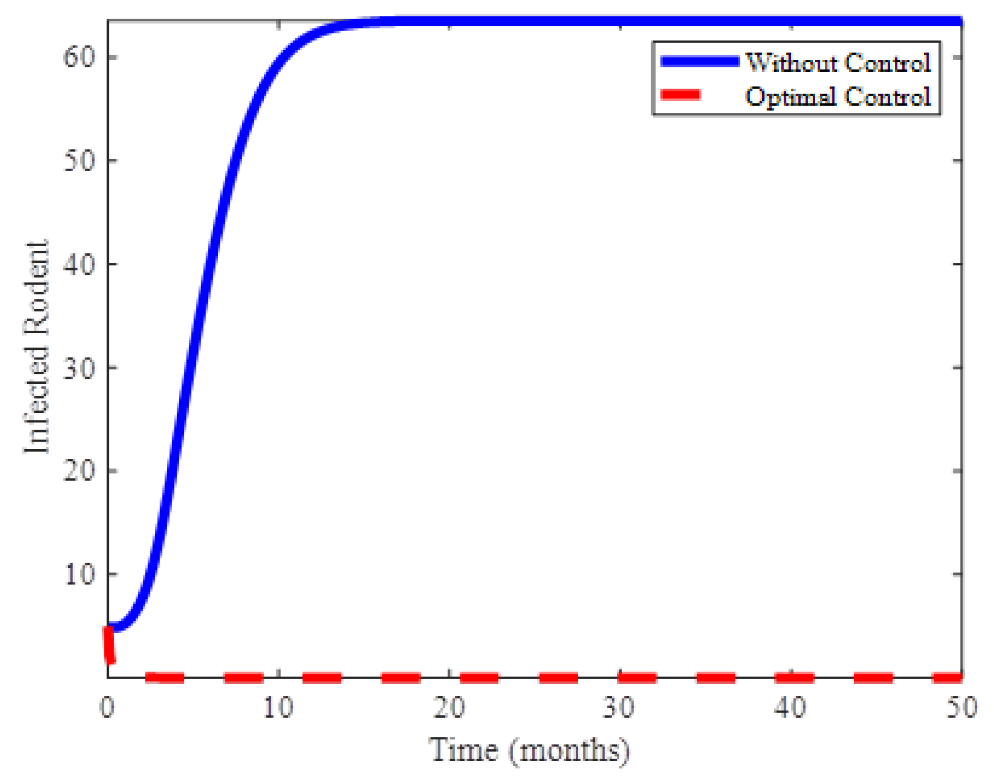
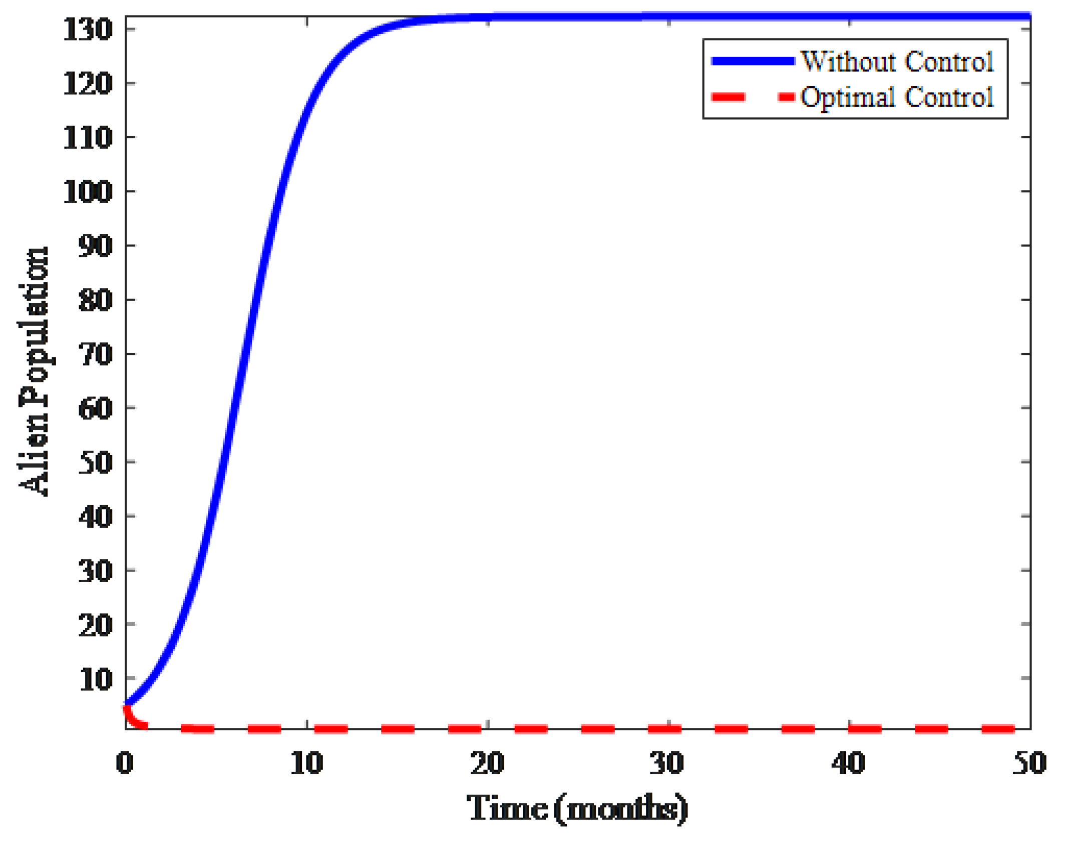
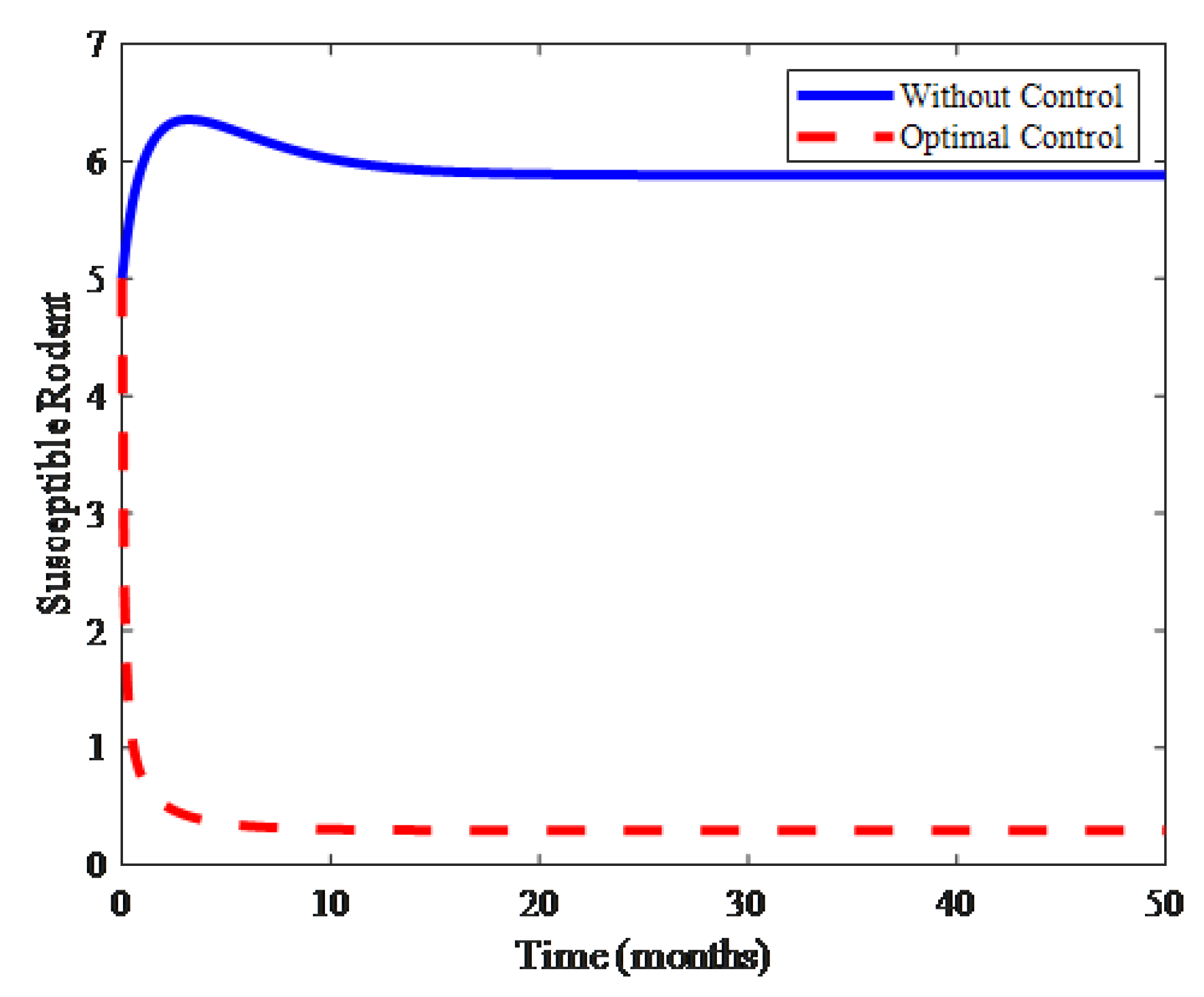
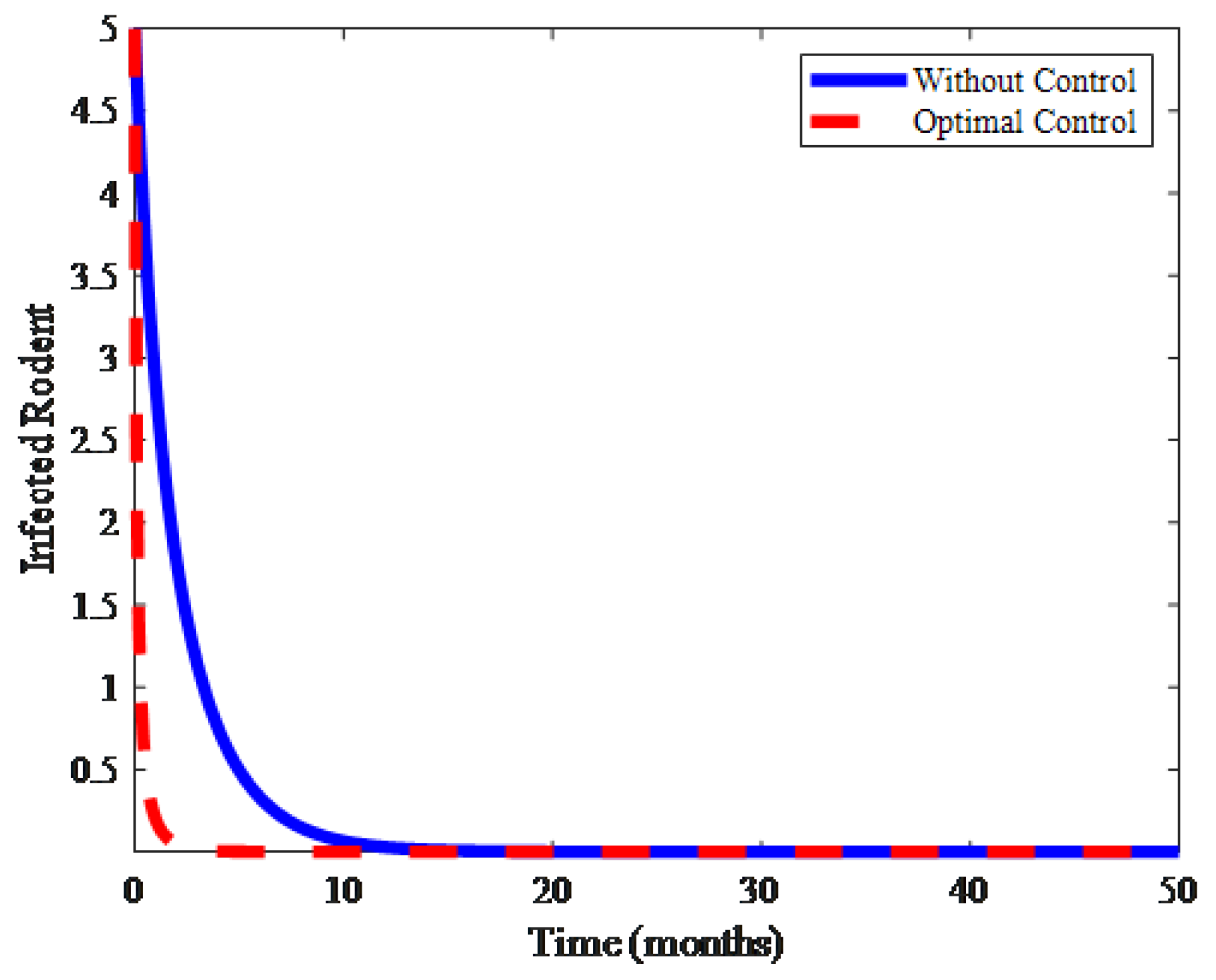
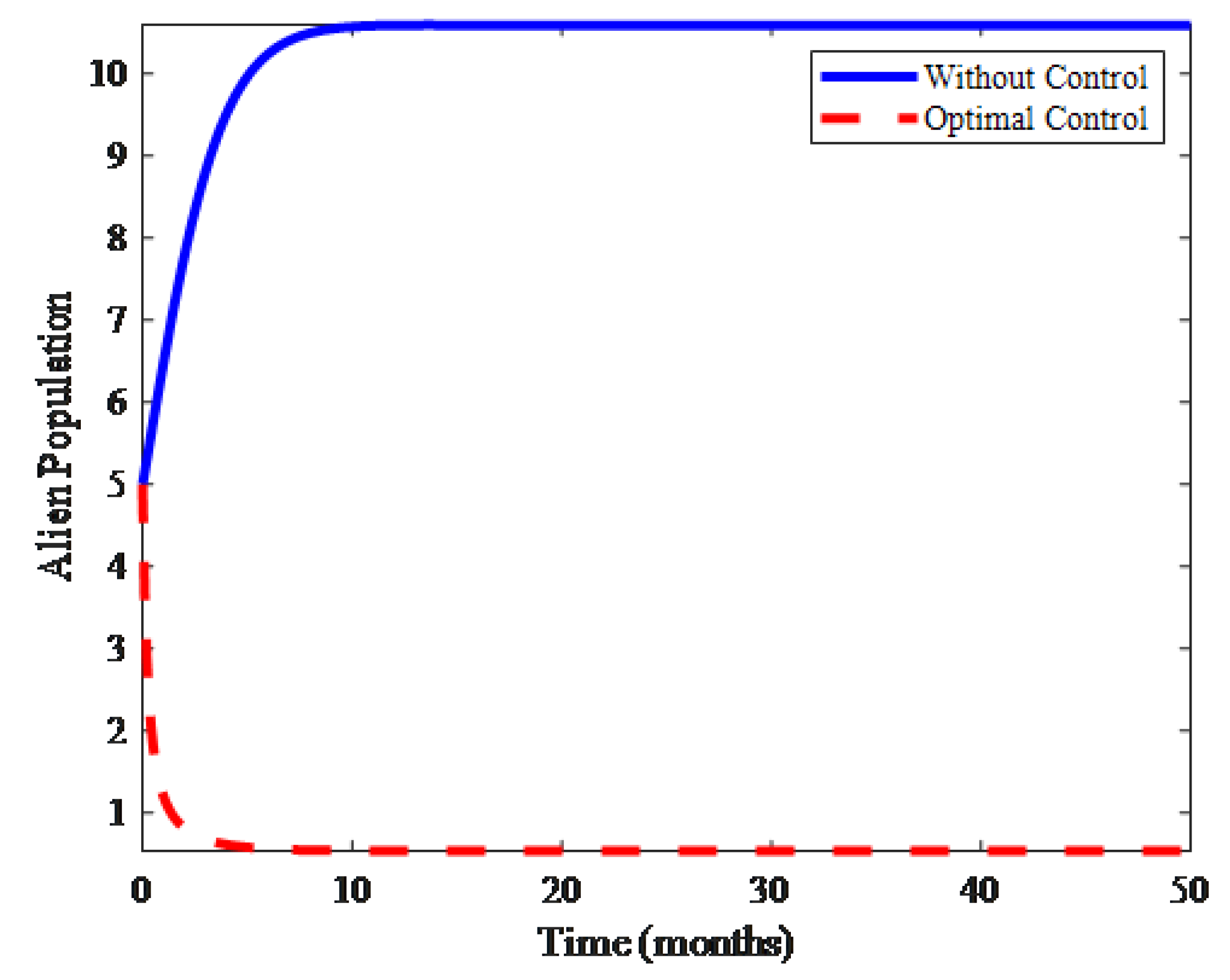
The dynamics of the models without optimum control (Equation (1)) and with optimum control (Equation (3)) are shown. Figure 1, Figure 2, and Figure 3 represent the susceptible rodent, infected rodent, and alien populations, respectively, in the two models, i.e., without control and with control. It is apparent in all of the figures that there are considerable differences between the number of rodents and alien populations under control as compared to cases without control.
In Figure 1, it can be observed that the susceptible rodent population r s will disappear and stabilize at a certain steady value when the two controls, i.e., harvesting efforts E ( t ) and biodiversity u ( t ) , are applied. The susceptible rodent population behaves in the opposite way in the model without optimum control, wherein it increases sharply initially and reaches a certain maximum, before plunging and approaching an equilibrium quantity.
For the optimum control model (Equation (3)), Figure 2 shows the number of infected rodents r i decreases strongly and drops to extinction thereafter, while the population of infected rodents r i thrives and approaches an equilibrium stable value for the model without optimum control (Equation (1)). The results illustrated in Figure 2 clearly show that the activated control strategy is effective in eliminating the infected rodent population with the presence of harvesting efforts E ( t ) and biodiversity u ( t ) as optimum control, which is not the case without control. The use of harvesting efforts E ( t ) and biodiversity u ( t ) can eliminate the number of infected rodents, and this indicates that the hantavirus infection will die off with the presence of two controls.
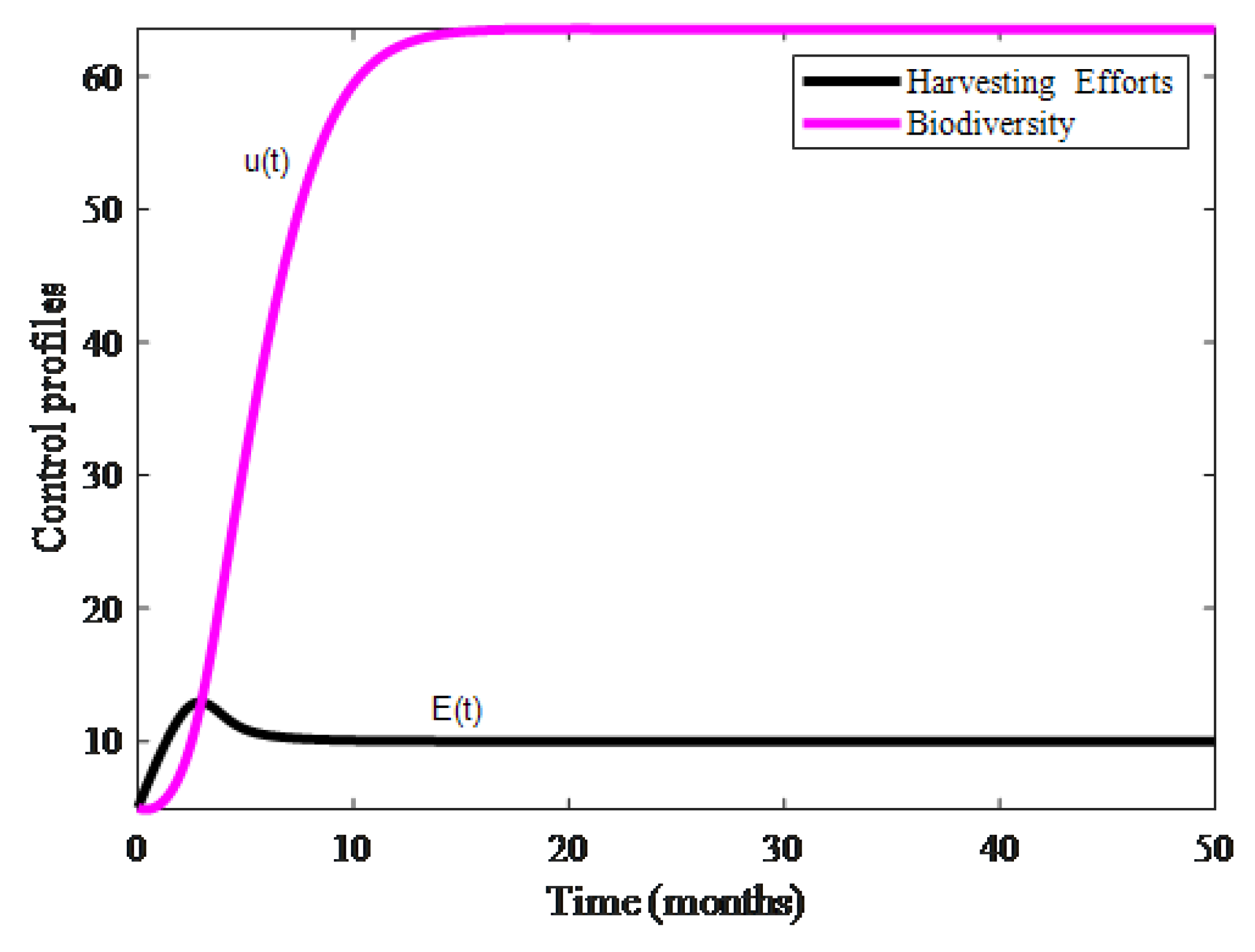
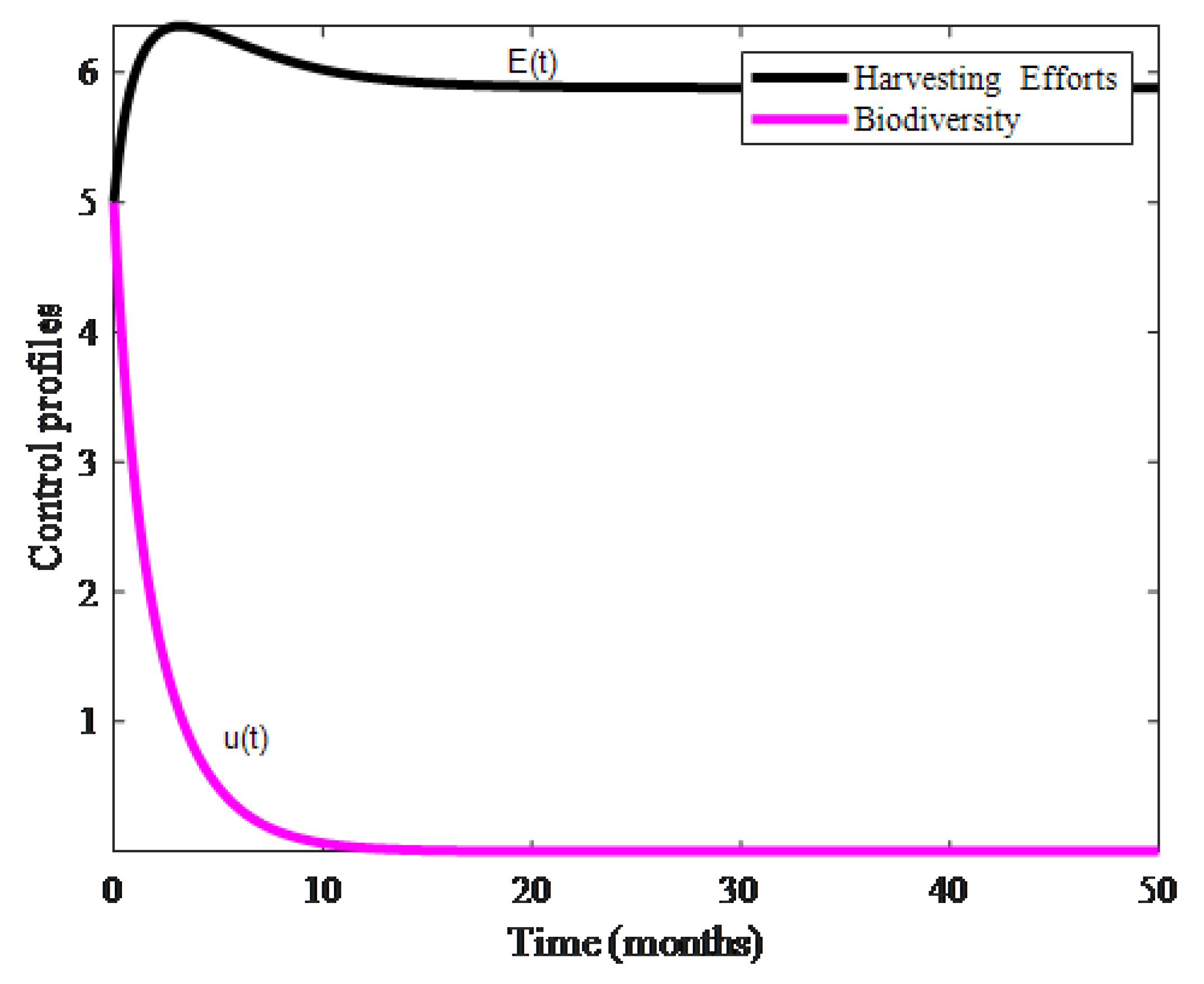
The numerical simulation results in Figure 3 display a similar pattern to Figure 2 for the models without control (Equation (1)) and with control (Equation (3)). When the optimum control model is considered, we observe that the population of alien z a decreases with a slower rate and eventually drops to extinction. In the model without optimum control, the alien population can survive and stabilize at a certain steady value. Figure 4 shows harvesting efforts E ( t ) and biodiversity u ( t ) as control variables. The optimum control increases in month 50, and a small population of susceptible rodents remains, while both the infected rodent and alien populations die off.
Next, we consider the simulation result as the environmental parameter, k, is decreased to 20. The results for k = 20 are as shown in Figure 5, Figure 6, Figure 7 and Figure 8. Note that initial conditions for case k = 20 are given by r s = 5 , r i = 5 , and z a = 5 . Figure 5 exhibits a similar transmission as Figure 1 as for the cases with and without control. In Figure 6, the illustrated result shows the number of infected rodents decreases strongly and drops to extinction. In this case, as the environmental parameter is decreased, the number of infected rodents in the system with no control will also drop to extinction, but at a slower rate compared to a system with control parameters. Figure 7 also shows similar trends to the result in Figure 2 but with a faster rate. In Figure 8, we show harvesting efforts and biodiversity as control variables. The optimum control for harvesting increases in month 50, while the biodiversity factor is reducing. A small population of susceptible rodents remains, while both the infected rodent and alien populations die off. Finally, the results from the two cases presented above indicate that effects on environmental capacity, such as availability of food sources, might also impact the spread of the infection.

5. Conclusions

In this paper, we studied the effects of the harvesting efforts E ( t ) and biodiversity u ( t ) as an optimum control on the spread of the hantavirus infection. First, we proposed a new mathematical model that takes into account the presence of an alien population and the hantavirus using optimum control theory. The theoretical studies of optimal control models and their numerical simulations are discussed in this paper. Then, the optimum controls are applied to minimize both populations of rodents. The results from this model clearly show that the optimum control is able to eliminate the infected rodent populations with the presence of harvesting efforts and biodiversity as the controls, as well as in the case without control.

Author Contributions

Writing—original draft preparation, F.M.Y.; methodology, analysis, F.M.Y.; review and editing, F.A.A., A.I.M.I.; funding acquisition, F.A.A.

Funding

This research was funded by Fundamental Research Grant Scheme (203.PMATHS.6711570) by Ministry of Higher Education, Malaysia and Bridging Grant (304.PMATHS.6316285) by Division of Research & Innovation (RCMO) – USM.

Acknowledgments

We would like to express our thank to the Faculty of Science and Mathematics, Sultan Idris Education University and the School of Mathematical Sciences, Universiti Sains Malaysia for providing computing assistance and facilities in this research.

Conflicts of Interest

The authors declare no conflict of interest. The funders had no role in the design of the study; in the collection, analyses, or interpretation of data; in the writing of the manuscript, or in the decision to publish the results.

References

  1. Raharinosy, V.; Olive, M.-M.; Andriamandimby, S.F.; Filippone, C.; Heraud, J.-M. Geographical distribution of Hantivarus identified from small terrestrial mammals in Madagascar and evaluation of risk factors relating to the Hantivarus infection. Int. J. Infect. Dis. 2018, 73, 386. [Google Scholar] [CrossRef]
  2. Guterres, A.; Sampaio de Lemos, E.R. Hantaviruses and a neglected environmental determinant. One Health 2018, 5, 27–33. [Google Scholar] [CrossRef] [PubMed]
  3. Koishi, A.C.; Aoki, M.N.; Jorge, T.R.; Suzukawa, A.A.; Zanluca, C.; Levis, S.; Duarte dos Santos, C.N. Development and validation of a point-of-care test for detecting Hantavirus antibodies in human and rodent samples. Diagn. Microbiol. Infect. Dis. 2016, 85, 323–327. [Google Scholar] [CrossRef]
  4. Avšič-Županc, T.; Saksida, A.; Korva, M. Hantavirus infections. Clin. Microbiol. Infect. 2019, 21, e6–e16. [Google Scholar] [CrossRef] [PubMed] [Green Version]
  5. Abramson, G.; Kenkre, V.M. Spatiotemporal patterns in the Hantavirus infection. Phys. Rev. E 2002, 66, 1912. [Google Scholar] [CrossRef] [Green Version]
  6. Abramson, G.; Kenkre, V.M.; Yates, T.L.; Parmenter, B.R. Traveling waves of infection in the Hantavirus epidemics. Bull. Math. Biol. 2003, 65, 519–534. [Google Scholar] [CrossRef]
  7. Giuggioli, L.; Kenkre, V.M.; Abramson, G.; Camelo-Neto, G. Theory of Hantavirus infection spread incorporating localized adult and itinerant juvenile mice. Eur. Phys. J. B 2006, 55, 461–470. [Google Scholar]
  8. Peixoto, I.D.; Abramson, G. The effect of biodiversity on the Hantavirus epizootic. Ecology 2006, 87, 873–879. [Google Scholar] [CrossRef] [Green Version]
  9. Abramson, G. Mathematical modeling of Hantavirus: From the mean field to the individual level. In Progress in Mathematical Biology Research; Kelly, J.T., Ed.; Nova Science Publishers Inc.: New York, NY, USA, 2008; pp. 1–27. [Google Scholar]
  10. Goh, S.M.; Ismail, A.I.M.; Noorani, M.S.M.; Hashim, I. Dynamics of the Hantavirus infection through variational iteration method (VIM). Nonlinear Anal. Real World Appl. 2009, 10, 2171–2176. [Google Scholar] [CrossRef]
  11. Rida, S.Z.; Abdel Rady, A.S.; M Arafa, A.A.; Khalil, M. The effect of the environmental parameter on the Hantavirus infection through a fractional-order SI model. Int. J. Basic Appl. Sci. 2012, 1, 88–99. [Google Scholar] [CrossRef] [Green Version]
  12. Yusof, F.M.; Ismail, A.I.M.; Ali, N.M. Modeling population harvesting of rodents for the control of Hantavirus infection. Sains Malays. 2012, 39, 935–940. [Google Scholar]
  13. Jasrasaria, R.; Mitra, D. The Effects of Intraspecific and Interspecific Competition on Plant Growth. 2004. Available online: http: //88.198.249.35/d/Effect-of-plant-population-density-on-growth-and-yield-of.pdf (accessed on 20 January 2015).
  14. Yusof, F.M.; Ismail, A.I.M.; Ali, N.M. Effect of predators on the spread of hantavirus infection. Sains Malays. 2014, 43, 1045–1051. [Google Scholar]
  15. Yusof, F.M.; Ismail, A.I.M.; Hasan, Y.A. Implication of Predator Interaction of the Spread of Hantavirus Infection. Matematika 2018, 34, 205–226. [Google Scholar] [CrossRef]
  16. Yusof, F.M.; Azmi, A.; Mohd, M.H.; Ismail, A.I.M. Effect of Biodiversity on the Spread of Leptospirosis Infection. In Proceedings of the International Conference on Mathematical Sciences and Technology 2018 (MathTech 2018), The Hotel Equatorial Penang, Malaysia, 10–12 December 2018. [Google Scholar]
  17. Hale, B.M.; McCarthy, M.L. An Introduction to Population Ecology—Harvesting a Population with Logistic Growth. Available online: https://www.maa.org/press/periodicals/loci/joma/an-introduction-to-population-ecology-harvesting-a-population-with-logistic-growth (accessed on 20 January 2015).
  18. Kar, T.K.; Pahari, U.K. Modelling and analysis of a prey-predator system with stage-structure and harvesting. Nonlinear Anal. Real World Appl. 2007, 8, 601–609. [Google Scholar] [CrossRef]
  19. Sion, M.L.; Hatzitolios, A.I.; Armenaka, M.C.; Toulis, E.N.; Kalampalika, D.; Mikoudi, K.D. Acute renal failure caused by Leptospirosis and Hantavirus infection in an urban hospital. Eur. J. Intern. Med. 2002, 13, 264–268. [Google Scholar] [CrossRef]
  20. Bryson, A.E., Jr. Optimal control-1950 to 1985. Control Systems. IEEE Control Syst. Mag. 1996, 16, 26–33. [Google Scholar] [CrossRef]
  21. Khan, M.A.; Islam, S.; Khan, S.A.; Khan, I.; Shafie, S.; Gull, T. Prevention of Leptospirosis Infected Vector and Human Population by Multiple Control Variables; Hindawi Publishing Corporation: New York, NY, USA, 2014; pp. 1–9, Abstract and Applied Analysis. ID 619035. [Google Scholar]
  22. Okosun, K.O.; Mukamuri, M.; Makinde, D.O. Global stability analysis and control of Leptospirosis. Open Math. 2016, 14, 567–585. [Google Scholar] [CrossRef] [Green Version]
  23. Lenhart, S.; Workman, J.T. Optimal Control Applied to Biological Models; Mathematical and computational Biology Series; Chapman and Hall: London, UK, 2007. [Google Scholar]
  24. Bonyah, E.; Okosun, K.O. Mathematical modeling of Zika virus. Asian Pac. J. Trop. Dis. 2016, 6, 673–679. [Google Scholar] [CrossRef]
  25. Pontryagin, L.S.; Boltyanskii, V.G.; Gamkrelidze, R.V.; Mishchenko, E. The Mathematical Theory of Optimal Processes (Translated by D.E. Brown) A Pergamon Press Book; The Macmillan Company: New York, NY, USA, 1964; pp. 56–57. [Google Scholar]
  26. Momoh, A.; Fügenschuh, A. Optimal control of intervention strategies and cost effectiveness analysis for a Zika virus model. Oper. Res. Health Care 2018, 18, 99–111. [Google Scholar] [CrossRef]
  27. Khan, M.A.; Zaman, G.; Islam, S.; Chohan, M.I. Optimal Campaign in Leptospirosis Epidemic by Multiple Control Variables. Appl. Math. 2012, 3, 1655–1663. [Google Scholar] [CrossRef] [Green Version]
  28. Lashari, A.A.; Zaman, G. Optimal control of a vector borne disease with horizontal transmission. Nonlinear Anal. Real World Appl. 2012, 13, 203–212. [Google Scholar] [CrossRef]
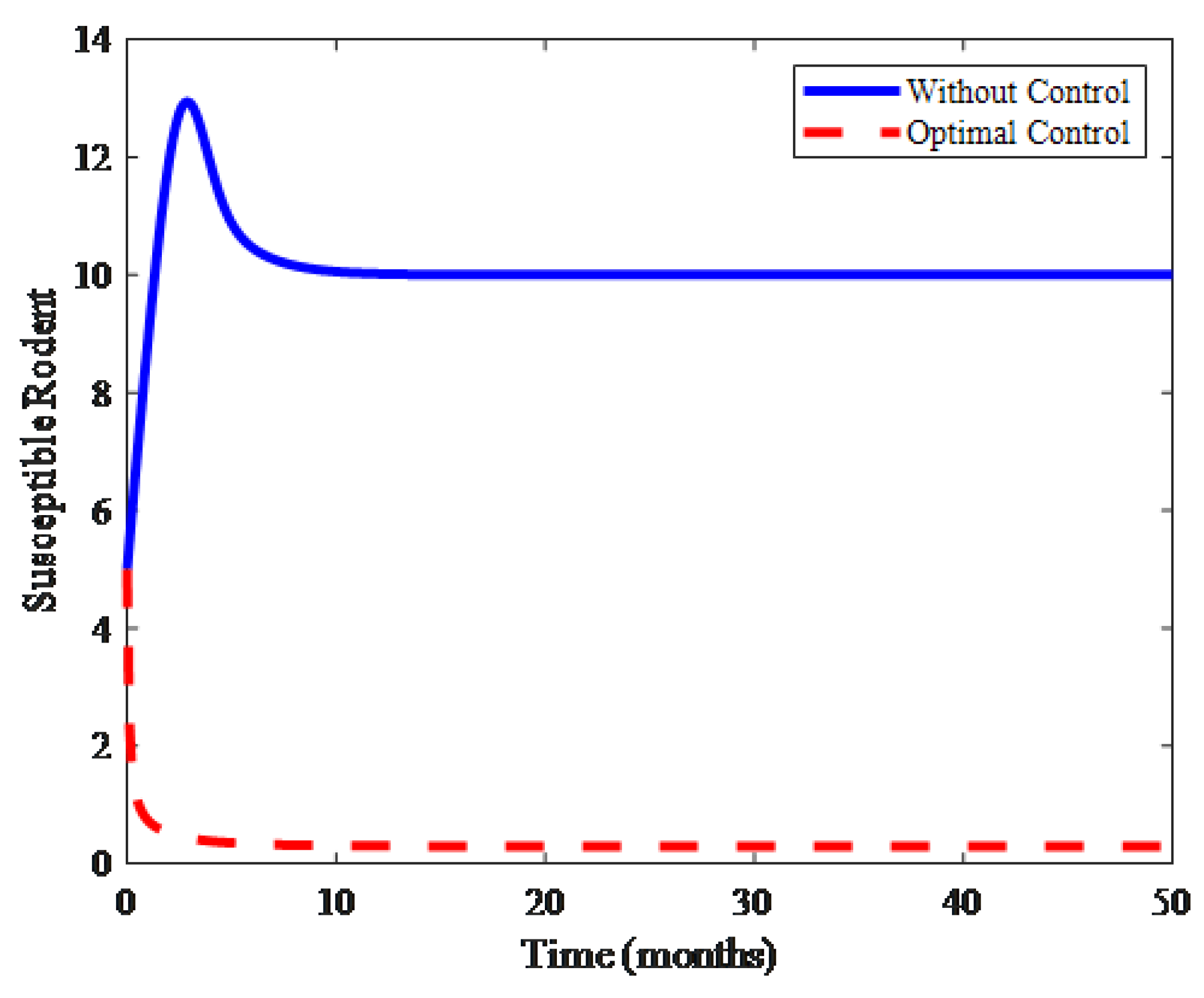
Figure 1. Value of susceptible rodent population r s without control (E(t) = 0 and u(t) = 0, given by Equation (1), and with control (Equation (3)), modeled with the initial values r s = 5 , r i = 5 , z a = 5 , and k = 250 .
Mathematics 07 01192 g001
Figure 2. Value of the infected rodent population r i without control (E(t) = 0 and u(t) = 0, given by Equation (1), and with control (Equation (3)), modeled with the initial values r s = 5 , r i = 5 , z a = 5 and k = 250 .
Mathematics 07 01192 g002
Figure 3. Value of the alien population z a without control (E(t) = 0 and u(t) = 0, given by Equation (1), and with control (Equation (3)), modeled with the initial values r s = 5 , r i = 5 , z a = 5 , and k = 250 .
Mathematics 07 01192 g003
Figure 4. The plot shows the harvesting efforts E ( t ) and biodiversity u ( t ) as control variables.
Mathematics 07 01192 g004
Figure 5. Value of susceptible rodent population r s without control (E(t) = 0 and u(t) = 0, given by Equation (1) and with control (Equation (3)), modeled with the initial values r s = 5 , r i = 5 , z a = 5 , and k = 20 .
Mathematics 07 01192 g005
Figure 6. Value of the infected rodent population r i without control (E(t) = 0 and u(t) = 0, given by Equation (1) and with control (Equation (3)), modeled with the initial values r s = 5 , r i = 5 , z a = 5 , and k = 20 .
Mathematics 07 01192 g006
Figure 7. Value of the alien population z a without control (E(t) = 0 and u(t) = 0, given by Equation (1), and with control (Equation (3)), modeled with the initial values r s = 5 , r i = 5 , z a = 5 and k = 20 .
Mathematics 07 01192 g007
Figure 8. The plot shows the harvesting efforts E ( t ) and biodiversity u ( t ) as control variables.
Mathematics 07 01192 g008
Table 1. Description of the parameters used in Equation (2).
SymbolDescription
b1The recruitment rate of human population
β1, β2The mediate transmission coefficients
λhThe immune human once again is susceptible at constant rate
μhThe natural mortality rate for human
δhThe disease related death rate from infected class occurs at human population
γhThe recovery rate for human from the infections
b2The recruitment rate for vector population
γvThe death rate of vector
β3The disease carrying of susceptible vector per host per unit time
δvThe disease death rate of vector populations
1, ∈2The rate of positive constants.
u1(t)Human should cover all cuts, water dry, full-cover boots, shoes and long sleeve shirts when handling animals
u2(t)Wash hands thoroughly on a regular basis and shower after work
u3(t)Clean up both work place and home
Table 2. Parameter values in the numerical simulations.
SymbolDescriptionParameter value
b The birth rate of rodent species1
c The death rate of rodent species0.6
a The transmission rate of hantavirus0.1
k The environmental parameterVaried
q Competitive effect of rodents on alien species0.2
β The birth rate of alien species1
  γ   The death rate of alien species0.5
  ε Competitive effect of rodents on alien species0.1
E ( t ) The harvesting effortsVaried
u ( t ) The biodiversityVaried