Construction of EMD-SVR-QGA Model for Electricity Consumption: Case of University Dormitory

Abstract

In the context of the nationwide call for “energy savings” in China, it is desirable to establish a more accurate forecasting model to manage the electricity consumption from the university dormitory, to provide a suitable management approach, and eventually, to achieve the “green campus” policy. This paper applies the empirical mode decomposition (EMD) method and the quantum genetic algorithm (QGA) hybridizing with the support vector regression (SVR) model to forecast the daily electricity consumption. Among the decomposed intrinsic mode functions (IMFs), define three meaningful items: item A contains the terms but the residual term; item B contains the terms but without the top two IMFs (with high randomness); and item C contains the terms without the first two IMFs and the residual term, where the first two terms imply the first two high-frequency part of the electricity consumption data, and the residual term is the low-frequency part. These three items are separately modeled by the employed SVR-QGA model, and the final forecasting values would be computed as A + B − C. Therefore, this paper proposes an effective electricity consumption forecasting model, namely EMD-SVR-QGA model, with these three items to forecast the electricity consumption of a university dormitory, China. The forecasting results indicate that the proposed model outperforms other compared models.

1. Introduction

The university dormitory is the place where college students spend most of their daily life. The electricity consumption is often huge without any saving actions. In the context of the nationwide call for “energy savings” in China, it is necessary to provide some effective education courses, guidance, and management approach to cultivate “energy savings” behavior (habit), and eventually to achieve the “green campus” policy. Therefore, it is desirable to establish a more accurate forecasting model to monitor electricity consumption particular from the university dormitory. However, the electricity consumption data of a university dormitory are influenced by lots of factors, such as weather conditions, holidays, population of the dormitory, social activities of university, energy policy of university, and so on [1,2], the electricity consumption data demonstrate the non-linearity in nature, which lead the electricity consumption forecasting work be more complicate [3,4].

In the past decades, many researchers proposed lots of electricity consumption forecasting models to receive more accurate forecasting results. These forecasting models are often divided into two categories [5]: the statistical methods and the artificial intelligent (AI) models. The statistical methods only employ historical data to find out the linear relationships among time periods. There are various statistical models that contain the ARIMA models [6,7,8], regression models [9,10,11], exponential smoothing models [12,13], Kalman filtering models [14,15], Bayesian estimation models [16,17], and so on. However, the inherent shortcomings of these statistical models are that they are only defined to deal with the linear relationships among the electricity consumption and other influenced factors mentioned above, eventually, only receiving unsatisfied forecasting results [18].

Along with advanced nonlinear computing ability, the AI models have been mature diffusely explored to improve the forecasting accuracy of electricity consumption since the 1980s, such as artificial neural networks (ANNs) [18,19,20,21,22], expert system models [23,24,25,26], and fuzzy inference methodologies [27,28,29,30]. To further overcome the inherent drawbacks embedded in these AI models, hybrid and combined models (hybridizing or combining with other advanced AI techniques) have received lots of attention [31,32,33,34,35,36,37,38,39], as mentioned in [5], three kinds of these hybrid or combined models, for example, hybridizing or combining these AI models with each other [31,32,33]; hybridizing or combining with the statistical models [34,35,36]; and hybridizing or combining with meta-heuristic algorithms [37,38,39]. It is recommended to employ any kind of hybrid or combined model to receive more satisfied forecasting results [40]. However, these AI models (containing hybrid or combined models) also have their inherent drawbacks from the theoretical mechanisms, such as difficult to determine the network structural parameters [41]; time-consuming to modeling [42]; easily trapped into a local minimum [43]; more insightful discussions of AI models in electricity consumption could be referred in [44].

As shown in the powerful nonlinear modeling performance, the support vector regression (SVR) model [45] has already been with abundant research results to deal with electric load forecasting [4,46,47,48,49]. Based on the conclusions of these papers, the well determination of parameters for an SVR model by any meta-heuristic algorithm could guarantee more satisfied forecasting accuracy. Among those employed meta-heuristic algorithms in the literature, the quantum genetic algorithm (QGA) proposed in [50] is considered to be employed in this paper, not only it is empowered by the quantum computing mechanism (QCM), but also it is a classic algorithm with mature applications to solve real problems [51,52]. On the other hand, it is also concluded in the literature that decomposing the time series by the empirical mode decomposition (EMD) method [53] into several single and apparent components (namely intrinsic mode functions (IMFs)), then, separately forecasting each component, it would eventually receive higher forecasting accuracy. The EMD method had also been applied in many fields [53,54,55]. Therefore, this paper would also apply the EMD method to extract the electricity consumption time series data into several IMFs, then, each IMF is forecasted by an SVR model with QGA, and the final forecasting results are summed by the forecasted value of each IMF.

However, as mentioned in [40], the decomposed IMFs contain IMFs with different randomness and the residual IMF; then, these IMFs should be separately modeled by the proposed forecasting model to receive superior forecasting performance. Inspired by the different randomness of IMFs, these two kinds of IMFs could have many combinations to obtain more accurate forecasting results. 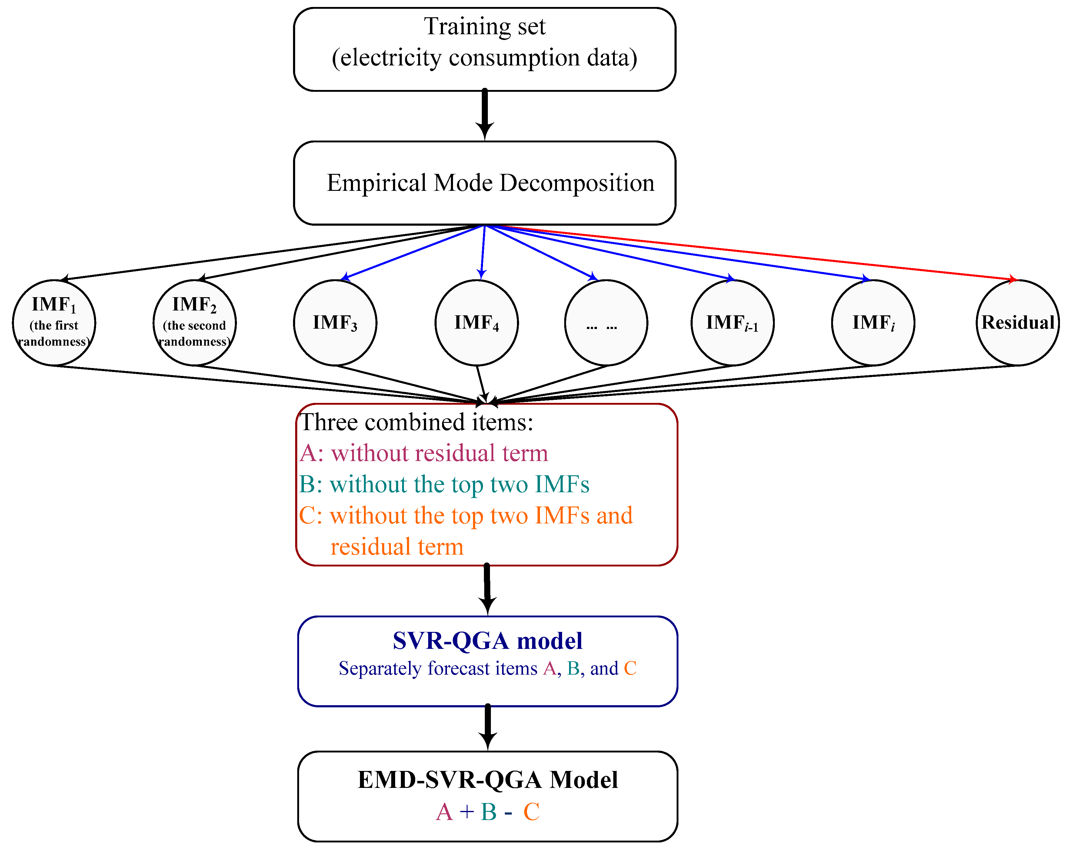Thus, based on the EMD method, the QGA, and the SVR model, the authors propose a new hybrid model, namely the EMD-SVR-QGA model, to compare the forecasting performance of different IMF combinations and different algorithms with the H-EMD-SVR-PSO model [40]. The electricity consumption data of a university dormitory is decomposed by the EMD method into six IMFs. Then, these decomposed IMFs are combined into three items: item A contains the terms minus the residual term, item B contains the terms minus the top two IMFs (with high randomness), and item C only contains the terms minus the top two IMFs and the residual term contents. Items A, B, and C would be separately modeled by the SVR-QGA model proposed in [50]. For item A, there are many IMFs with different randomness, which implies that it can have neutral volatility while the SVR-QGA modeling. For item B, the residual term could be fine-tuned under the remaining IMFs (with low randomness), it is also fine while the SVR-QGA modeling. For item C, it is complete with low randomness, which is excellent during the SVR-QGA modeling. Finally, the electricity consumption forecasting results are calculated by the forecasting values of A + B − C. The forecasting details would be presented in the following sections.

To compare the forecasting performance among the proposed EMD-SVR-QGA model and other compared models, the original SVR model, the SVR-QGA model (hybridizing the QGA algorithm with an SVR model), and the H-EMD-SVR-PSO model [40], the electricity consumption data are collected from a university dormitory, Quanshan Campus, Jiangsu Normal University, China, with daily type, from 1 September 2018 to 31 March 2019. The experimental results indicate the superiority of the proposed EMD-SVR-QGA model in terms of forecasting accuracy.

The remainder of this paper is organized as follows. The proposed EMD-SVR-QGA model is introduced in Section 2. The numerical example against other alternative models is illustrated in Section 3. The conclusion is shown in Section 4.

2. The Proposed EMD-SVR-QGA Model

2.1. The Empirical Mode Decomposition (EMD) Method

The EMD [53] method is an adaptive time series decomposition method to decompose the original time series with its inherent characteristics into several different stationary IMFs. Each IMF should satisfy the following two criteria: (1) in the whole time range, each IMF at most has one extreme value over; and (2) the mean value of two envelopes by the local maxima and local minima should be zero at any point. Therefore, the EMD method can theoretically overcome the premature convergent problem. For the original time series, $x\left(t\right)$, the decomposition procedures of the EMD method are demonstrated as follows.

Step 1: calculation of the mean envelope. Apply the cubic spline interpolation to connect all maxima and minima identified in $x\left(t\right)$, to find out the upper envelope and lower envelope, respectively. The mean envelope, $n_1$, is calculated by the average value of the upper envelope and the lower envelope.

Step 2: decomposing. The first IMF candidate, $d_1$, is the difference between $n_1$ and the original signal $x\left(t\right)$, as shown in Equation (1),

$$d_1=x\left(t\right)-n_1.$$

(1)

Check whether $d_1$ meets the two criteria of an IMF mentioned above. If $d_1$ does not satisfy, then, $d_1$ would be viewed as the original data set, and $n_1$ would be zero. Then, repeat the above evolution procedure for k times, the k-th component, $d_{1k}$, is shown as by Equation (2),

$$d_{1k}=d_{1\left(k-1\right)}-n_{1k}.$$

(2)

where $d_{1k}$ and $d_{1\left(k-1\right)}$ represent the data set after k times and k − 1 times evolution procedures, respectively.

Step 3: identify IMF. If $d_{1k}$ meets the two criteria of an IMF, then, $d_{1k}$ can be identified as the first IMF component, $IM{F}_1$. A new series, $d_1^{\prime }$, by subtracting IMF₁ (as Equation (3)), would continue the decomposition procedure.

$$d_1^{\prime }=x\left(t\right)-IM{F}_1$$

(3)

Step 4: IMF composition. Repeat steps 1 to 3, until the remained $x\left(t\right)$ becomes a monotone function, i.e., there are no new IMFs decomposed from $d_n^{\prime }$. The decomposition details of these $n$ IMFs are shown in Equation (4). As shown in Equation (5), the series, $d_n^{\prime }$, is the remainder of x(t), i.e., the residual of $x\left(t\right)$.

$$\begin{gathered} d_1^{\prime }=x\left(t\right)-IM{F}_1 \\ {d}_2^{\prime }=d_1^{\prime }-IM{F}_2 \\ {d}_n^{\prime }=d_{n-1}^{\prime }-IM{F}_n \end{gathered}$$

(4)

$$x\left(t\right)={\displaystyle \sum }_{i=1}^{n}IM{F}_i+d_n^{\prime }.$$

(5)

2.2. Hybrid Support Vector Regression with Quantum Genetic Algorithm (SVR-QGA) Model

2.2.1. Support Vector Regression Model

The modeling details of the SVR-QGA model are briefly illustrated as follows. For a given nonlinear electricity consumption data set, ${\left\{\left(x_i,y_i\right)\right\}}_{i=1}^N$ (where $x_i$ represents the actual electricity consumption data) is mapped into a high dimensional feature space by a non-linear mapping function, $\phi \left(x\right)$, where the so-called SVR function, $f\left(x\right)$, as shown in Equation (6), is theoretically to formulate the nonlinear relationship between the input training data ($x_i$) and the output data ($y_i$).

$$y=f\left(x\right)=w^T\phi \left(x\right)+b,$$

(6)

where $f\left(x\right)$ represents the forecasted values; the weight, w, and the intercept, b, can be computed during the SVR modeling process.

Based on the SVR theory, the empirical risk minimization problem can be transformed to solve the quadratic optimization problem with inequality constraints as shown in Equation (7),

$$\underset{\mathrm{w},b,\xi ,{\xi }^{*}}{\mathrm{Min}}R\left(\mathrm{w},\xi ,{\xi }^{*}\right)=\frac{1}{2}\Vert \mathrm{w}{\Vert }^2+\mathrm{C}{\displaystyle \sum }_{i=1}^N\left({\xi }_i+{\xi }_i^{*}\right),$$

(7)

with the constraints:

$$\begin{array}{c}\mathrm{w}\phi \left(x_i\right)+b-f\left(x_i\right)\le \epsilon +{\xi }_i^{*},\\ -\mathrm{w}\phi \left(x_i\right)-b+f\left(x_i\right)\le \epsilon +{\xi }_i,\\ {\xi }_i^{*},{\xi }_i\ge 0\\ i=1,2,\dots ,N,\end{array}$$

where $\frac{1}{2}\Vert \mathrm{w}{\Vert }^2$ is used to maximize the distance of two separated training data, it also determines the steepness and the flatness of $f\left(x\right)$; C is a parameter to penalize the training errors; ε is the width of the ε-insensitive loss function, which defines the loss is zero only if the forecasting value is within the range of ε; two positive slack variables, $\xi$ and ${\mathsf{\xi }}^{*}$, are used to represent the training statuses, training error above ε, denotes as ${\xi }^{*}$, training error below –ε, denotes as $\xi$.

The constrained optimization problem (Equation (7)) can be solved by using the following primal Lagrangian form, as shown in Equation (8),

$$\begin{gathered} L\left(\mathrm{w},\mathrm{b},{\xi }_i,{\xi }_i^{*},{\alpha }_i,{\alpha }_i^{*},{\beta }_i,{\beta }_i^{*}\right) \\ =\frac{1}{2}\Vert \mathrm{w}{\Vert }^2+\mathrm{C}{\displaystyle \sum }_{i=1}^N\left({\xi }_i+{\xi }_i^{*}\right)-{\displaystyle \sum }_{i=1}^N{\beta }_i^{*}\left[f\left(x_i\right)-\mathrm{w}\phi \left(x_i\right)-b+\epsilon +{\xi }_i^{*}\right] \\ -{\displaystyle \sum }_{i=1}^N{\beta }_i\left[\mathrm{w}\phi \left(x_i\right)+b-f\left(x_i\right)\epsilon +{\xi }_i\right]-{\displaystyle \sum }_{i=1}^N\left({\alpha }_i{\xi }_i+{\alpha }_i^{*}{\xi }_i^{*}\right). \end{gathered}$$

(8)

Equation (8) is minimized with respect to primal variables $\mathrm{w},\mathrm{b},{\xi }_i,{\xi }_i^{*}$, and maximized with respect to nonnegative Lagrangian multipliers ${\alpha }_i,{\alpha }_i^{*},{\beta }_i,{\beta }_i^{*}$. Thus, Equations (9)–(12) are calculated.

$$\frac{\partial L}{\partial \mathrm{w}}=\mathrm{w}-{\displaystyle \sum }_{i=1}^N\left({\beta }_i-{\beta }_i^{*}\right)\phi \left(x_i\right)=0$$

(9)

$$\frac{\partial L}{\partial b}={\displaystyle \sum }_{i=1}^N\left({\beta }_i^{*}-{\beta }_i\right)=0$$

(10)

$$\frac{\partial L}{\partial {\xi }_i}=C-{\beta }_i-{\alpha }_i=0$$

(11)

$$\frac{\partial L}{\partial {\xi }_i^{*}}=C-{\beta }_i^{*}-{\alpha }_i^{*}=0.$$

(12)

Then, the KKT conditions are applied to the regression, Equation (7) would yield the dual Lagrangian by substituting Equations (9)–(12) into Equation (8). The dual Lagrangian, Equation (13), can be computed.

$$\mathcal{H}\left({\beta }_i,{\beta }_i^{*}\right)={\displaystyle \sum }_{i=1}^{N}f\left(x_i\right)\left({\beta }_i-{\beta }_i^{*}\right)-\epsilon {\displaystyle \sum }_{i=1}^N\left({\beta }_i+{\beta }_i^{*}\right)+\frac{1}{2}{\displaystyle \sum }_{i=1}^N{\displaystyle \sum }_{i=1}^N\left({\beta }_i-{\beta }_i^{*}\right)\left({\beta }_i-{\beta }_i^{*}\right)K\left(x,x_i\right),$$

(13)

with the constraints:

$${\displaystyle \sum }_{i=1}^N\left({\beta }_i-{\beta }_i^{*}\right)=0.$$

After solving the quadratic problem, Equation (7), the solution of the weight, w, in Equation (6) is computed by Equation (14),

$$\mathrm{w}={\displaystyle \sum }_{i=1}^N\left({\beta }_i-{\beta }_i^{*}\right)\phi \left(x_i\right),$$

(14)

where ${\beta }_i$ and ${\beta }_i^{*}$ are the Lagrangian multipliers.

Eventually, the SVR forecasting function is calculated as Equation (15),

$$f\left(x\right)={\displaystyle \sum }_{i=1}^N\left({\beta }_i-{\beta }_i^{*}\right)K\left(x,x_i\right)+b,$$

(15)

where $K\left(x_i,x_j\right)$ is the so-called kernel function, and its value could be computed by the inner product of $\phi \left(x_i\right)$ and$\phi \left(x_j\right)$, i.e., $K\left(x_i,x_j\right)=\phi \left(x_i\right)·\phi \left(x_j\right)$. Due to superior ability to mapping nonlinear data into high dimensional space, the Gaussian function (as shown in Equation (16)), is employed in this study. Therefore, there are totally three parameters, ε, σ and C, to be optimized in the modeling processes of the Gaussian kernel-based SVR model, to successfully improve the forecasting accuracy.

$$K\left(x_i,x_j\right)=\exp \left(-\frac{\Vert x_i-x_j{\Vert }^2}{2{\mathsf{\sigma }}^2}\right).$$

(16)

For comparison with Hong and Fan [40], this paper uses the QGA algorithm to look for suitable parameters of the SVR model.

2.2.2. Quantum Genetic Algorithm (QGA)

Genetic algorithm (GA) is a well-known effective evolutionary algorithm with its advanced operations, including selection, crossover, and mutation operations. It has been applied to solve many optimization problems. However, the worst shortcoming is that its population diversity would decrease along with repeated iterative computation and leads to some problems such as time-consuming, slow convergence, and trapping into local optima. Recently, the quantum computing mechanism [50,56,57] has been applied to be hybridized with the genetic algorithm [50]. The principal quantum computing mechanism, such as qubit, quantum superposition, and quantum entanglement are used to represent the chromosome of QGA into the qubit coding; eventually, the quantum rotation gate is also employed to renew the chromosomes in the modeling process. Therefore, it is with much superiority in faster convergent speed, time-saving, high diversity of population, and robustness.

The quantum computing mechanism is briefly introduced. The smallest information unit in the quantum system is called as qubit (the quantum bit), which demonstrates its state “0”, or “1”, or any superposition of these two states. The state of a qubit can be as Equation (17),

$$|\psi \rangle ={\alpha }_1|0\rangle +{\alpha }_2|1\rangle ,$$

(17)

where $|0\rangle$ and $|1\rangle$ represent the values of bits 0 and 1, respectively; ${\alpha }_1$ and ${\alpha }_2$ are the probability of the corresponding states and satisfy the normalization criterion, as illustrated in Equation (18),

$${\left|{\alpha }_1\right|}^2+{\left|{\alpha }_2\right|}^2=1.$$

(18)

The probability of a qubit individual as a string with $n$ qubits is presented as Equation (19),

$$q=\left[\begin{array}{c}{\alpha }_1\\ {\beta }_1\end{array}|\begin{array}{c}{\alpha }_2\\ {\beta }_2\end{array}|\begin{array}{c}\cdots \\ \cdots \end{array}|\begin{array}{c}{\alpha }_i\\ {\beta }_i\end{array}|\begin{array}{c}\cdots \\ \cdots \end{array}|\begin{array}{c}{\alpha }_n\\ {\beta }_n\end{array}\right],$$

(19)

where ${\left|{\alpha }_i\right|}^2+{\left|{\beta }_i\right|}^2=1$, $i=1,2,\dots ,n$.

Then, the chromosome with $n$ qubits is presented as, $Q=\left(q_1,q_2,\dots ,q_n\right)$, where $q_i\left(i=1,2,\dots ,n\right)$ denotes an individual qubit as shown in Equation (19). The quantum gate is an operator used for qubits to make the unitary transformations. In general, this operation is often presented by matrices. To obtain more results, it is feasible to use the trigonometric function with a rotation angle$\theta$, which is so-called quantum rotation gate, as shown in Equation (20). It is used to update as a better state.

$$Q^{\prime }=\left[\begin{array}{cc}\cos \theta & -\sin \theta \\ \sin \theta & \cos \theta \end{array}\right]Q,$$

(20)

where $Q^{\prime }$ is the updated chromosome; $\theta$ is the rotation angle.

2.2.3. Modeling Processes of QGA

The modeling processes of the SVR-QGA model are completely stated as follows.

Step 1: initialization. Three parameters of an SVR model are initialized as three genes to form a quantum chromosome with a string of m qubits (i.e., the superposition of all possible states), as shown in Figure 1. Based on the practical experiences in [50], a gene contains more qubits could be associated with better partitioning around the space, i.e., could obtain higher forecasting performances. Thus, in this paper, to receive more accurate forecasting results, the chromosome is initialized with 150 qubits (for each gene is 50 bits, i.e., m = 150). The population is initialized by setting all superposition states of qubits with equal amplitude as $\frac{1}{\sqrt{2}}$ [51].

Step 2: objective fitness evaluation. The objective fitness is evaluated by the quantum chromosome. For convenience, the principal forecasting accuracy index, the mean absolute percentage error (MAPE), as shown in Equation (21), is used to evaluate the objective fitness.

$$MAPE(\%)=\frac{1}{N}{\displaystyle \sum }_{i=1}^N\left|\frac{y_i-{\widehat{y}}_i}{y_i}\right|\times 100,$$

(21)

where N is the number of forecasts; $y_i$ is the actual value for forecast point i; ${\widehat{y}}_i$ is the forecast of point i.

Step 3: selection. The elitist selection is employed to select the best chromosome, which is with the smallest MAPE value during iterations of a generation. The selected elitist is set as the prior chromosome for the next generation.

Step 4: quantum crossover. To maintain the diversity of the population, the quantum crossover operation is used. This paper also uses the single-point-crossover to implement the crossover operation by two randomly selected chromosomes with crossover probability, P_cr, which is suggested to be set as 0.9 [50].

Step 5: quantum mutation. To efficiently enrich the diversity of the population, the quantum mutation operation is also employed. Each selected quantum chromosome will be changed by other suitable oscillation amplitudes (${\alpha }_i$,${\beta }_i$) of the corresponding state with the mutation probability, P_m, which is suggested to be set as 0.1 [50].

Step 6: quantum rotation. To avoid premature convergence, it is useful to change the quantum location of a qubit, therefore, the quantum rotation is used to modify the oscillation ranges of the qubit. The quantum rotation gate (shown in Equation (20)) with the rotation angle, $\theta$, is practically applied to perform the quantum rotation. The rotation angle, $\theta$, is corresponding to (${\alpha }_i$,${\beta }_i$) to modify the quantum location of a qubit. The values of $\theta$ are suggested to be between 0.1$\mathsf{\pi }$ and 0.005$\mathsf{\pi }$ [52].

Step 7: stop criteria. If the required number of generations is reached, then, the best solution is identified as the last quantum chromosome, else, go back to Step 3 to continue the three operations for the next generation.

2.3. The Complete Processes of the Proposed EMD-SVR-QGA Model

The complete processes of the proposed EMD-SVR-QGA model are presented in Figure 2 and stated as following steps.

Step 1: conduct decomposition of the training data. The electricity consumption data from the university dormitory would be decomposed by the EMD method into several characterized IMFs. These decomposed IMFs would be combined into three items: item A includes all IMFs but without the residual term; item B includes IMFs without top two (the first randomness and the second randomness which are with highly random, as shown in Figure 2) and the residual term; item C includes IMFs without top twos.

Step 2: defined items modeled by the SVR-QGA model. These three defined items, A, B, and C, are separately modeled by the SVR-QGA model. The modeling processes of the SVR-QGA model, such as quantum chromosome setting, superposition states of qubits, population initialization, selection operation, quantum crossover operation, quantum mutation operation, and quantum rotation operation, could refer Section 2.2.3 to learn about more details of the SVR-QGA model.

Step 3: final forecasting results. The final electricity consumption forecast is calculated by the values of these three items, A, B, and C, modeled separately by their corresponding SVR-QGA models. The calculation formula is easily given by the forecasts of A + B − C.

3. Electricity Consumption Forecasting by the EMD-SVR-QGA: Case of a University Dormitory

3.1. Data Set of Experimental Examples

The electricity consumption data are collected from a real-world case, two representative university dormitories, Quanshan Campus, Jiangsu Normal University, China. The detailed background of these data is stated as follows. There are about 12 persons per dormitory room. On the campus, each week about 10 seminars and associated lectures, each seminar or lecture would attract about 200 persons. The relative weight of Dormitories’ consumption in the corresponding university campus total consumption is about 14.78%. Based on the time period of the collected data, the associated weather is in fall and winter, as the campus is located in northern China, the official heating system is available. However, if suffering from heavy snow or intense cold, the electrical heater is also used. Thus, the electricity consumption would be moderate fluctuated along with the weather conditions. Finally, due to “energy savings” activities in China, the administration department also announces some active policy to encourage “energy savings”, eventually, to achieve the “green campus”, such as record merits, award, and give honorary title, etc.

It would be further processed by the proposed EMD-SVR-QGA model to receive the forecasting electricity consumption of these two selected dormitories in the future for one month. For these two dormitories, the electricity consumption data are both collected, with daily type, from 1 September 2018 to 31 March 2019, thus, each data set contains 212 electricity consumption data. However, during the vacation period, such as the Chinese Lunar Year Festival and the winter vacation, the electricity consumption of each dormitory is almost zero, i.e., these data should be removed. Therefore, after pre-processing operation, these two data sets from two dormitories are arranged to 110 and 134 electricity consumption data, respectively.

For clear denotation of these two dormitory cases, the first dormitory with 110 electricity consumption data is denoted as dormitory I, the other one with 134 electricity consumption is denoted as dormitory II. For the division of the training and the testing sets, Dormitory I is with 88 and 22 electricity consumption data in the training and the testing sets, respectively; dormitory II is with 107 and 27 electricity consumption data in the training and the testing sets, respectively.

Besides two dormitory cases, the electric load data set, collected from New South Wales (NSW) market in Australia also used in [40], is also employed to demonstrate the superiority of the proposed EMD-SVR-QGA model. The employed electric load data is collected from 1 to 13 August 2019, based on half-hour format, i.e., there are 48 data per day. The training set is from 1 to 10 August 2019 (in total 480 load data points), and the testing data is from 10 to 13 August 2019 (in total 144 load data points).

During the training stage of the SVR-QGA model, the rolling-based process [58,59], is employed to help QGA to systematic look for suitable parameter combination of an SVR model with smaller forecasting error. Specifically, the first n electricity consumption data is fed into the SVR-QGA model to conduct the model training process, then, the (n + 1)-th forecast value of electricity consumption and the feasible parameter combination are both obtained by the SVR-QGA model. Repeat this operation to receive the (n + 2)-th, the (n + 3)-th, … forecast values of electricity consumption till the required forecasting values are received. Finally, the parameter combination with the smallest testing errors are verified as the most appropriate parameter combination of an SVR model. Eventually, the testing data set will be used to compute the forecasting accuracy of the proposed SVR-QGA model.

3.2. Parameters Setting of the EMD-SVR-QGA Model

The parameters of QGA for these two dormitory cases are set practically or by referencing other experiences, the population scale (P_scale) is set to be 200 [50]; the generations of the population (q_max) are no larger than 200; the qubit string length of a quantum chromosome (m) is set as 150; the probabilities of quantum crossover (P_cr) and quantum mutation (P_m) are set as 0.5 and 0.1 [50], respectively. The rotation angle, $\theta$, is between 0.1$\mathsf{\pi }$ and 0.005$\mathsf{\pi }$ [52]. For SVR-QGA modeling, the maximal iteration for each example is all set as 10,000 in each generation; the searching range of the three parameters are set as followings, $\mathsf{\sigma }\in \left[0,10\right]$, $\mathsf{\epsilon }\in \left[0,1\right]$, and $C\in \left[0,200\right]$ in both two dormitory cases; δ is fixed as 0.001 [50].

3.3. Forecasting Accuracy Indexes and Forecasting Performance Superiority Test

To compare the forecasting accuracy among the proposed model and other compared models, four forecasting accuracy indexes, the mean absolute percentage error (MAPE), the root mean squared error (RMSE), mean squared error (RMSE), and the mean absolute error (MAE) is employed to calculate the forecasting errors, they are defined as Equations (21)–(24).

$$RMSE=\sqrt{\frac{{{\displaystyle \sum }}_{i=1}^N{\left(y_i-{\widehat{y}}_i\right)}^2}{N}}$$

(22)

$$MSE=\frac{{{\displaystyle \sum }}_{i=1}^N{\left(y_i-{\widehat{y}}_i\right)}^2}{N}$$

(23)

$$MAE=\frac{{{\displaystyle \sum }}_{i=1}^N\left|y_i-{\widehat{y}}_i\right|}{N},$$

(24)

where N is the number of forecasts; $y_i$ is the actual value for forecast point i ${\widehat{y}}_i$ is the forecast of point i.

On the other hand, it is necessary to conduct the statistical test to verify the statistical significance of the forecasting superiority of the proposed model. Based on Derrac et al. [60] suggestions, only Wilcoxon signed-rank test is implemented in this paper. The statistic of Wilcoxon signed-rank, W, is defined as Equation (25),

$$W=\min \left\{number(+),number(-)\right\},$$

(25)

where $number(+)$ is the total number of positive rank that the forecasting error of the proposed EMD-SVR-QGA model larger than other compared model; $number(-)$ is the total number of negative rank that the proposed EMD-SVR-QGA model smaller than the compared model.

If the value of W satisfies the required value of Wilcoxon distribution with an associated degree of freedom, then, the null hypothesis of equal performance of these two compared models is not accepted. It also reveals the outstanding forecasting results of the proposed EMD-SVR-QGA model outperforms significantly the compared model.

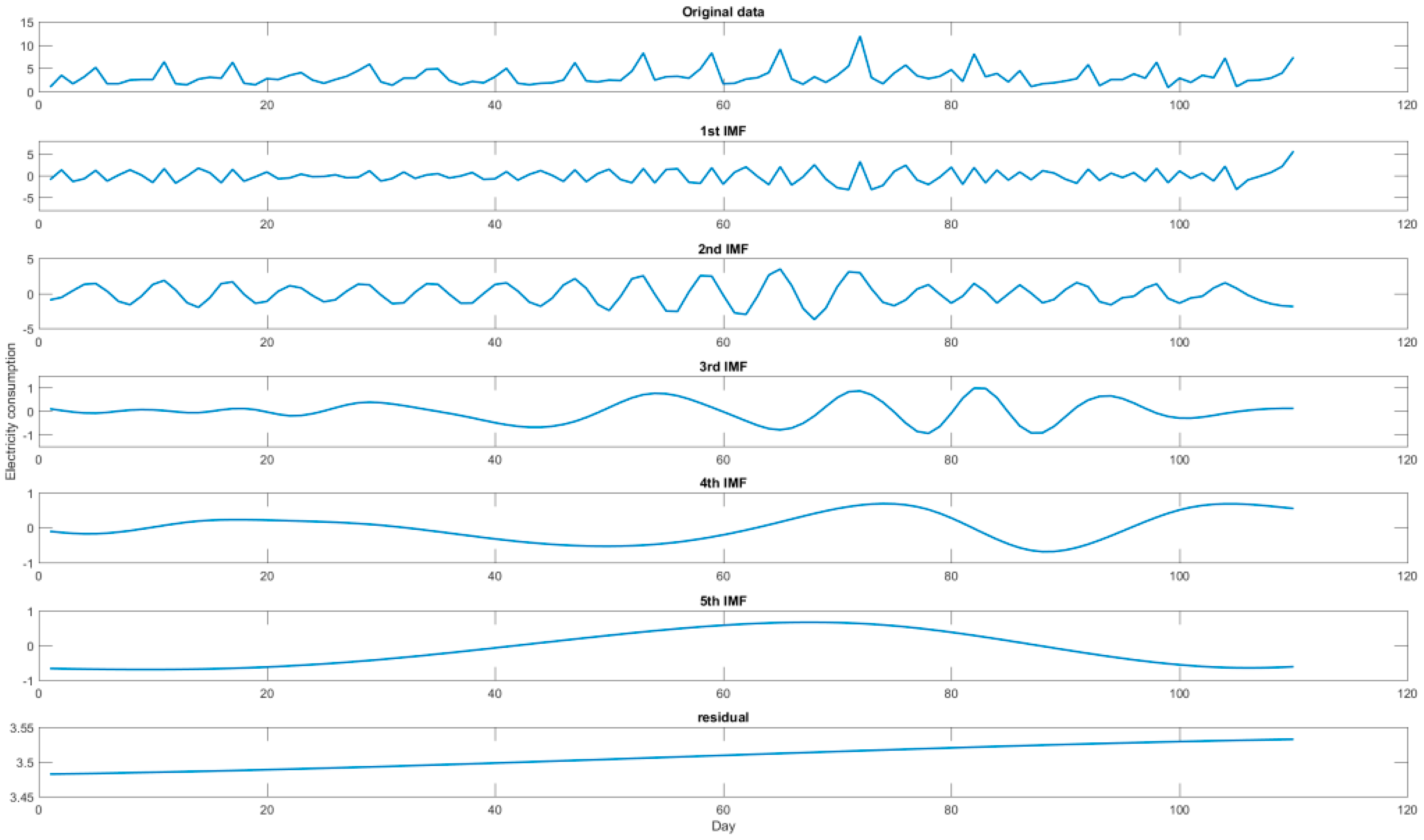
3.4. Decomposition Results and Forecasting Results for Dormitory I

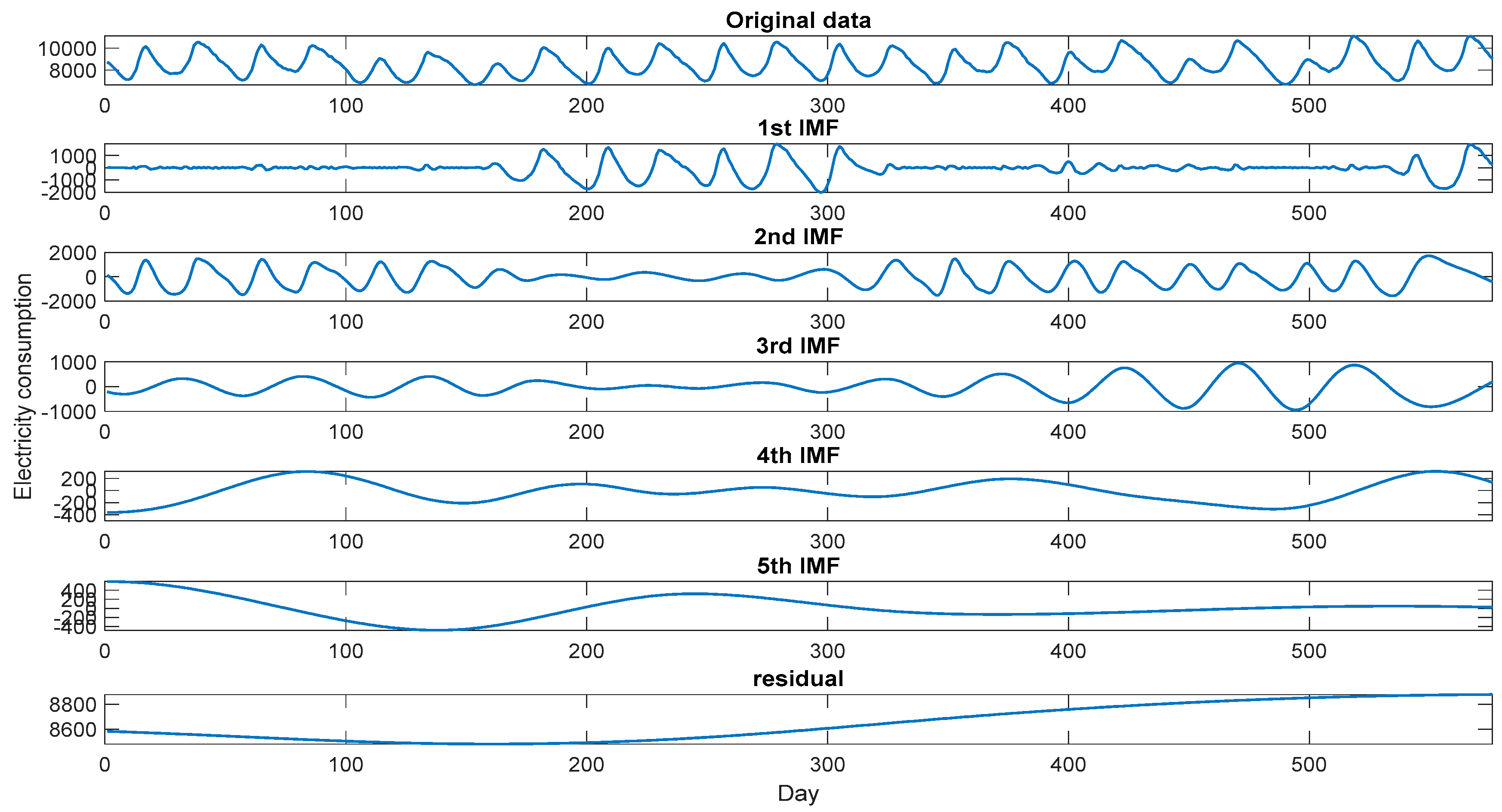
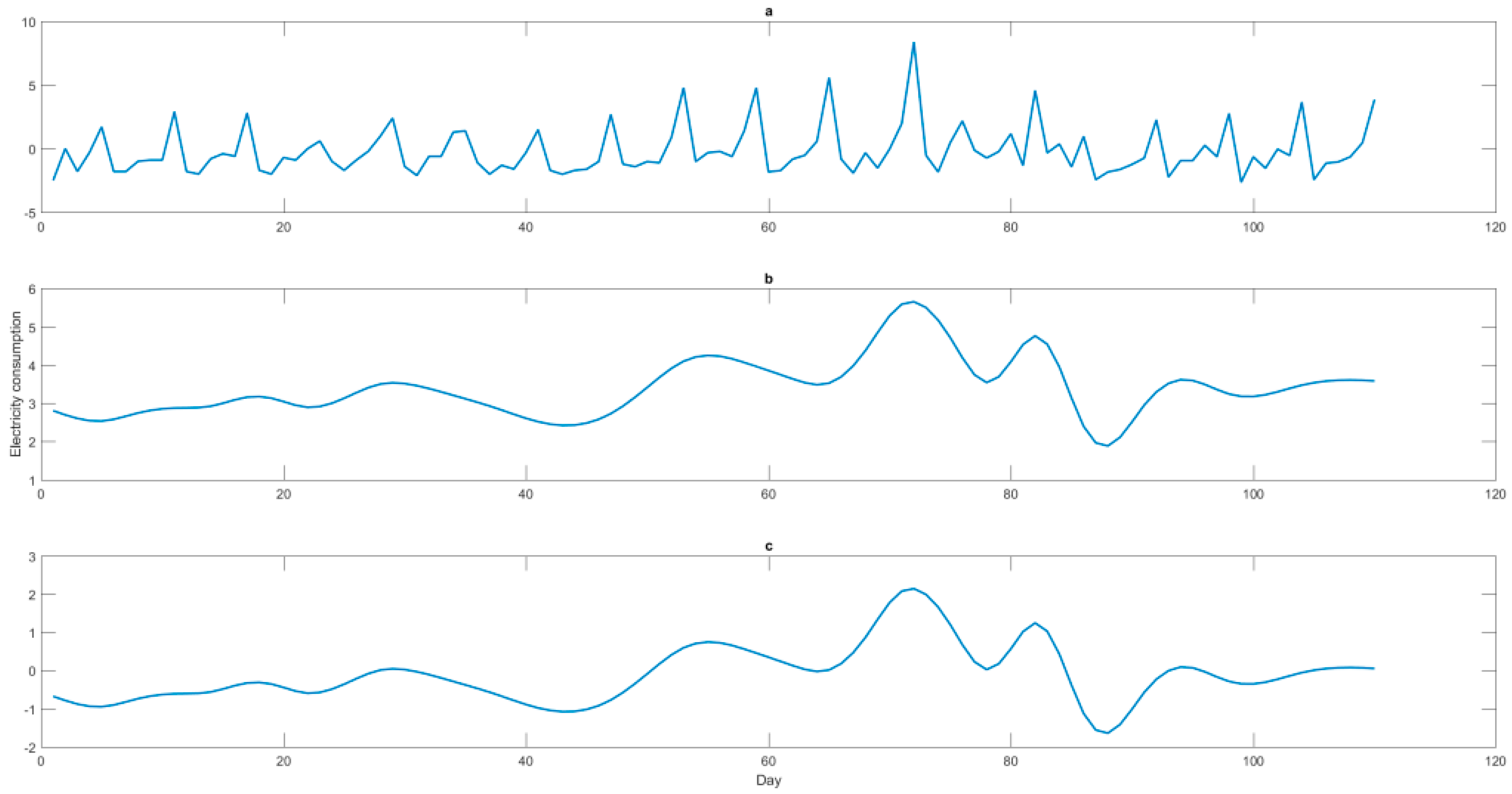
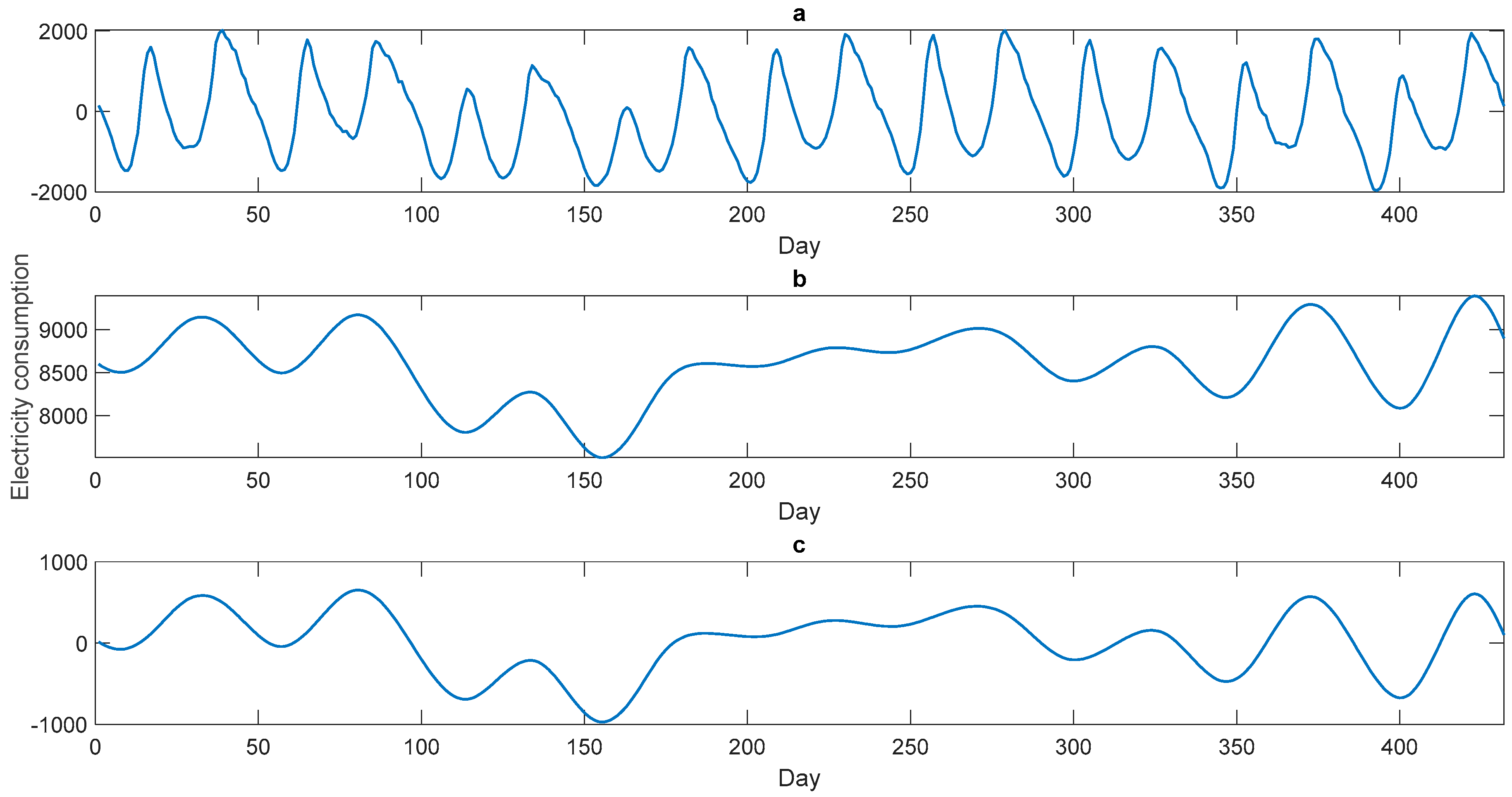
For Dormitory I case, the electricity consumption data is firstly decomposed by the EMD method into six terms. These six decomposed terms are demonstrated in Figure 3, in which the first IMF and the second IMF are obviously the random terms, the 6th IMF is also obviously the residual term. The three items A, B, and C, defined by the six IMFs are shown in Figure 4.

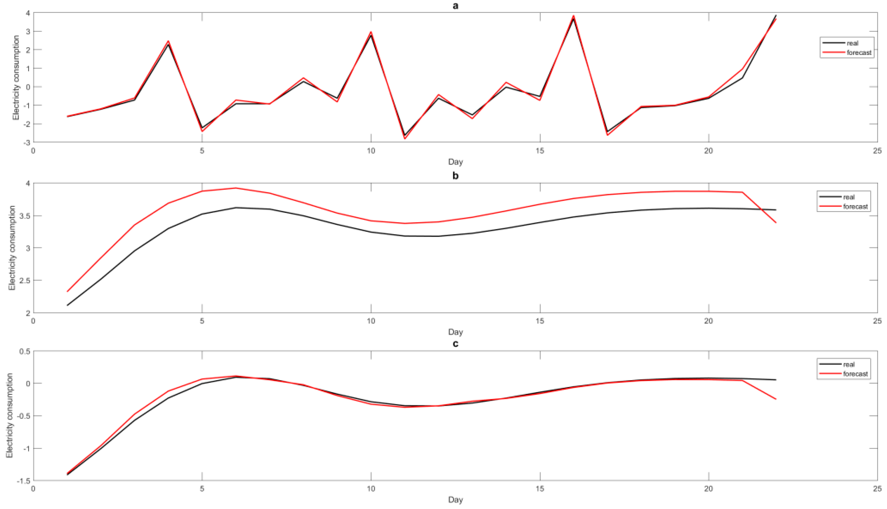
The three items A, B, and C, defined by the six IMFs are separately modeled by the SVR-QGA model, as mentioned in Section 3.1, the rolling-based process [58] is applied to collaborate with the QGA to determine the most appropriate parameter combination of their associated SVR-based models in the training phase. The appropriate parameter combination for each item is shown in

Table 1. The parameters of the EMD-SVR-QGA model and other compared models in dormitory I case.

Compared Models and Defined Items	Parameter Combination of the SVR Model
	$\mathit{\sigma }$	C	$\mathit{\epsilon }$
The original SVR model	3.00	100.00	0.50
The SVR-QGA model	2.83	96.86	0.58
The H-EMD-SVR-PSO model [40]
Item A: the random term + the middle term	0.14	89.00	0.0022
Item B: the middle term + the trend (residual) term	0.14	88.00	0.0020
Item C: the middle term	0.15	91.00	0.0025
The EMD-SVR-QGA model
Item A: all terms—the trend (residual) term	0.22	1.04	0.0574
Item B: all terms—top two IMFs	0.36	9.23	0.0683
Item C: all terms—top two IMFs—the trend (residual) term	0.40	9.40	0.0302

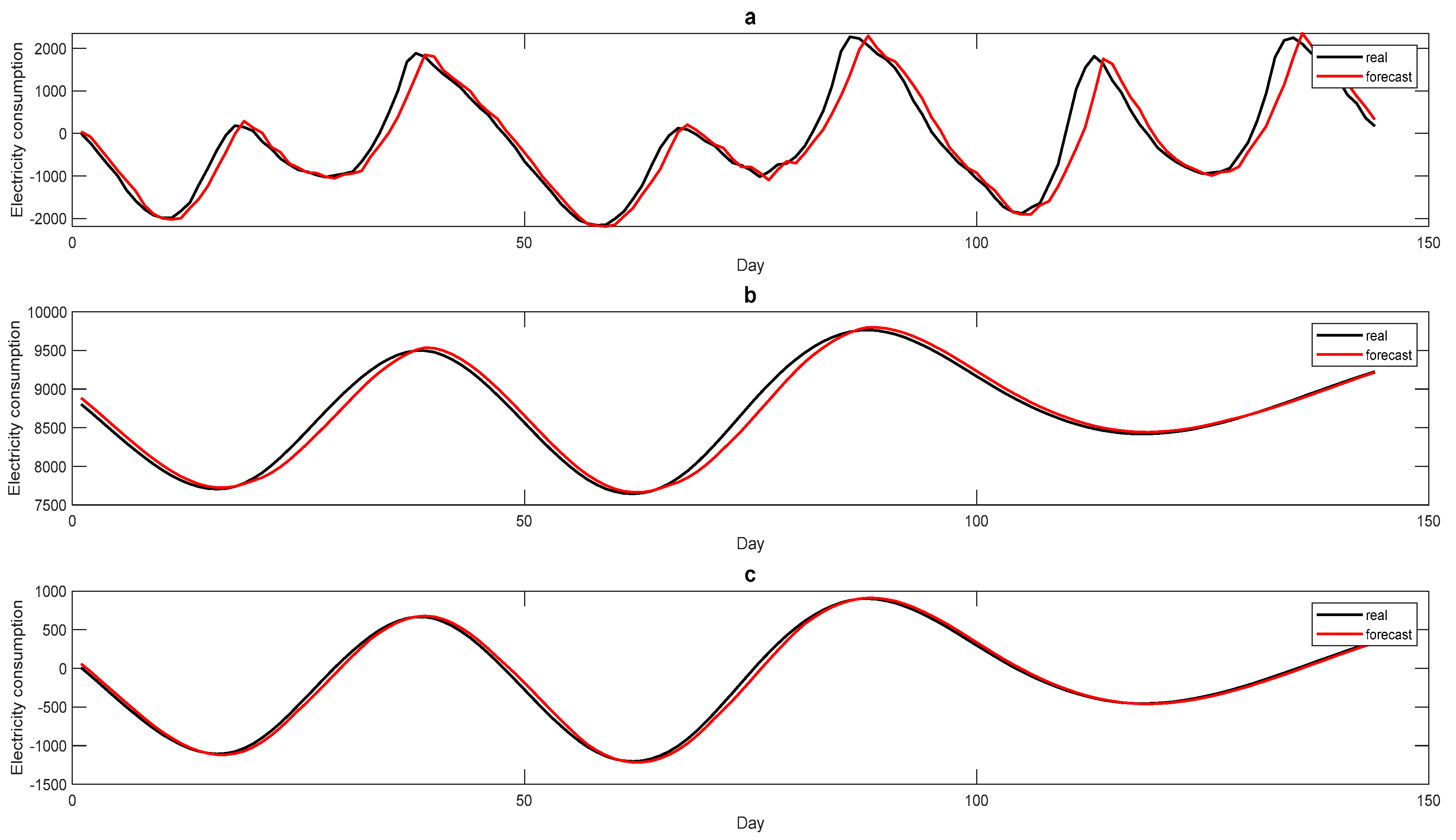
. In addition, the appropriate parameter combination for other compared models, including the original SVR model, the SVR-QGA model, the H-EMD-SVR-PSO model [40], are also illustrated in Table 1. The forecasting performances for the three items are demonstrated in Figure 5.

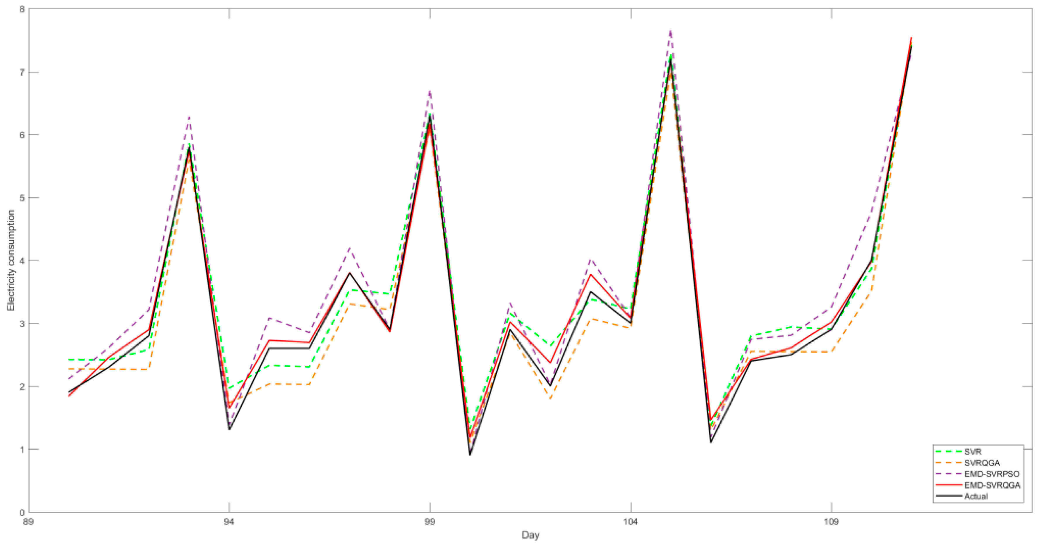
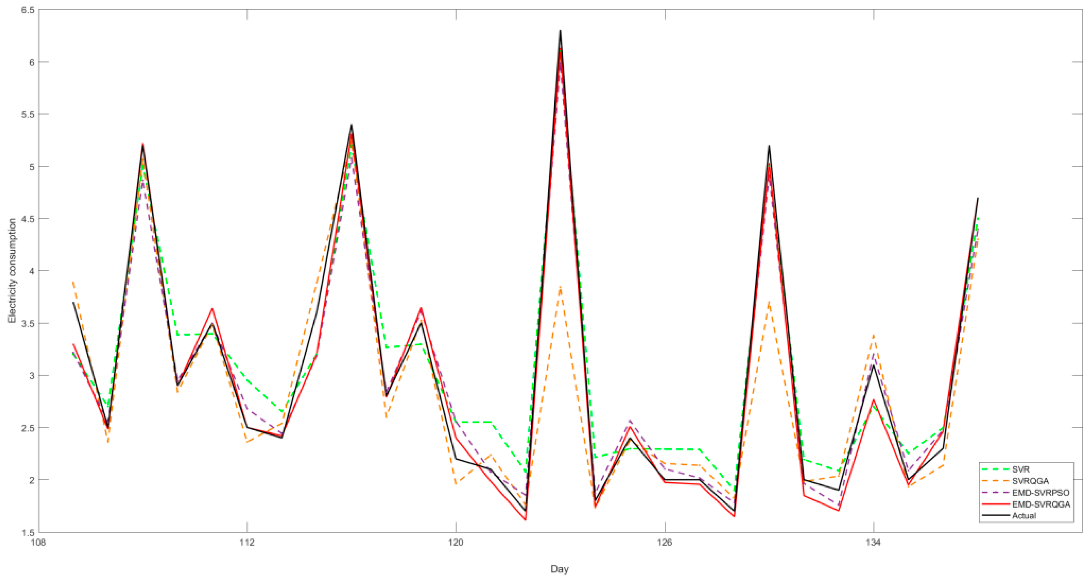
The forecasting results of the original SVR model, the SVR-QGA model [50], the H-EMD-SVR-PSO model [40], and the proposed EMD-SVR-QGA model are shown in Figure 6. It illustrates the forecasting curve of the proposed EMD-SVR-QGA model has better fitting effects than other compared models. It also implies that the proposed EMD-SVR-QGA model has the potentials to capture the fluctuation variation of the electricity consumption from this dormitory. Thus, the consumption behaviors can be effectively monitored and some valuable activities regarding improving electricity consumption habits can be held to successfully save electricity consumption.

The proposed EMD-SVR-QGA model also demonstrates better generalization ability than other models. The forecasting performance of these models is listed in

Table 2. Forecasting performance for the EMD-SVR-QGA and other compared models in the dormitory I case.

Compared Models	MAPE	RMSE	MSE	MAE
The original SVR	13.73	0.34	0.11	0.27
The SVR-QGA [50]	11.44	0.33	0.11	0.28
The H-EMD-SVR-PSO [40]	9.48	0.36	0.13	0.30
The EMD-SVR-QGA	7.40	0.18	0.03	0.14

. In which, it demonstrates clearly that the proposed EMD-SVR-QGA model outperforms the original SVR model, the SVR-QGA model [50], and the H-EMD-SVR-PSO model [40] in terms of four employed forecasting accuracy indexes. Particularly, for the H-EMD-SVR-PSO model, it also receives outstanding forecasting results, which indicates the forecasting advantages from this kind of EMD-SVR-based model. Comparing the forecasting accuracy of the EMD-SVR-QGA model and the H-EMD-SVR-PSO model, their contributions are different due to different combination types of these decomposed IMFs and the residual term. Therefore, looking for a suitable IMFs combination approach is an interesting research topic.

In addition, in Table 2, it also can see that the forecasting accuracy of the SVR-QGA model [50] is not superior to the EMD-SVR-based models. This is because the nonlinear effects are inherent in the electricity consumption data itself, and demonstrate the interactions among the IMFs and the residual term. After decomposition operation by the EMD method, the EMD-SVR-based models are able to well deal with this inherent non-linear data pattern by the IMFs and these defined items, A, B, and C. Therefore, the proposed EMD-SVR-QGA model can be a useful forecasting model to deal with the electricity consumption forecasting work of a university dormitory.

Finally, to verify the significant contribution of the forecasting improvement from the proposed EMD-SVR-QGA model, in this paper, the Wilcoxon signed-rank test is suggested [59]. Wilcoxon signed-rank test is conducted on one-tail-test, under two significant levels, α = 0.025 and α = 0.05. The test results are shown in

Table 3. Wilcoxon signed-rank test for the dormitory I case.

Compared Models	Wilcoxon Signed-Rank Test
	α = 0.025; W = 65	α = 0.05; W = 75
EMD-SVR-QGA vs. Original SVR	5 *	5 *
EMD-SVR-QGA vs. SVR-QGA	7 *	7 *
EMD-SVR-QGA vs. H-EMD-SVR-PSO	10 *	10 *

Note: * denotes that the EMD-SVR-QGA model significantly outperforms other compared models.

, which obviously indicate that the proposed EMD-SVR-QGA model is significantly superior to other compared models.

3.5. Decomposition Results and Forecasting Results for Dormitory II

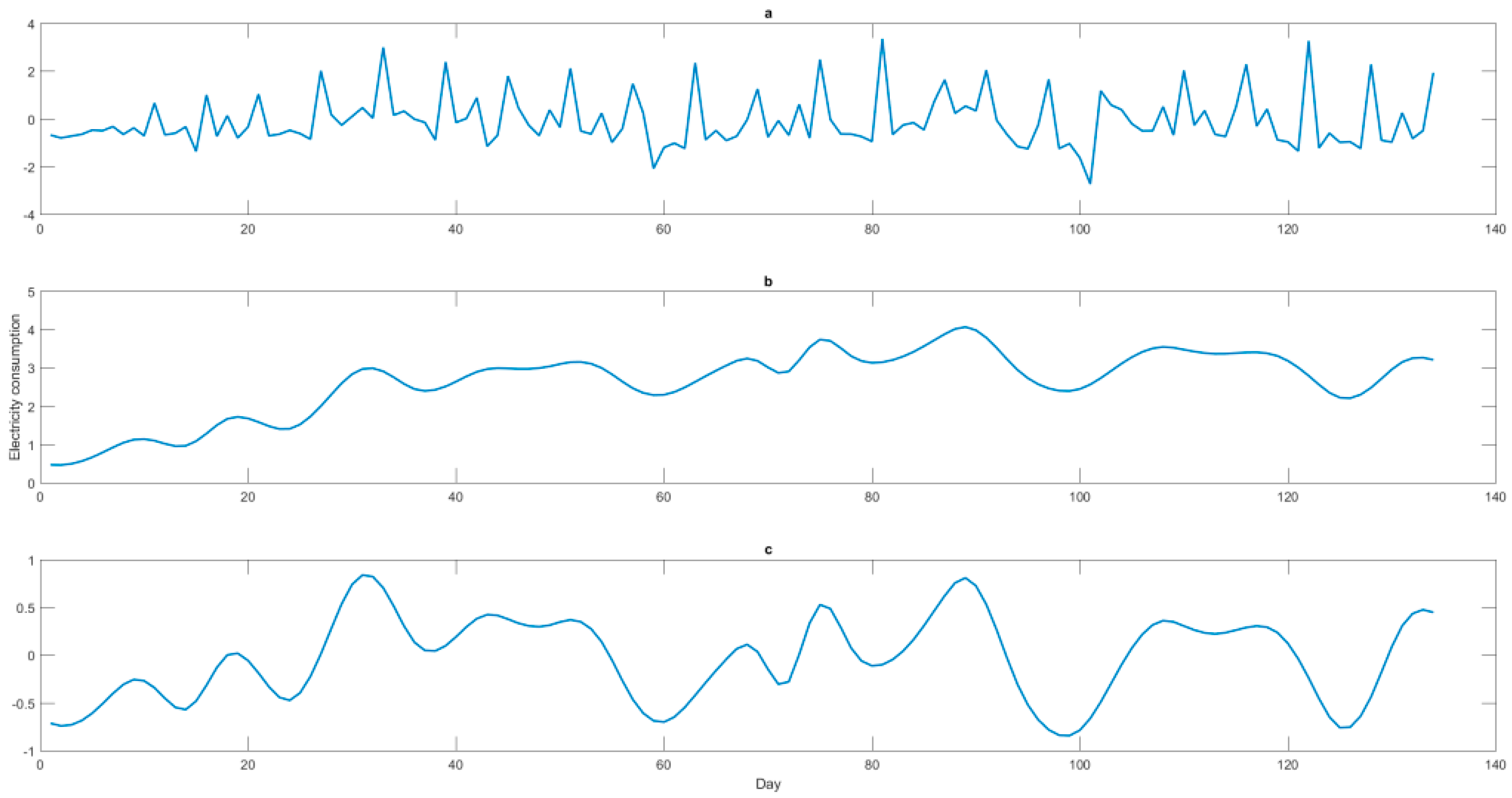
Similar to the dormitory I case, the electricity consumption data in the dormitory II case is also firstly decomposed by the EMD method into six terms. These six decomposed terms are demonstrated in Figure 7, in which the 1st IMF and the 2nd IMF are obviously the random terms, the 6th IMF is also obviously the residual term. The three items A, B, and C, defined by the six IMFs are shown in Figure 8.

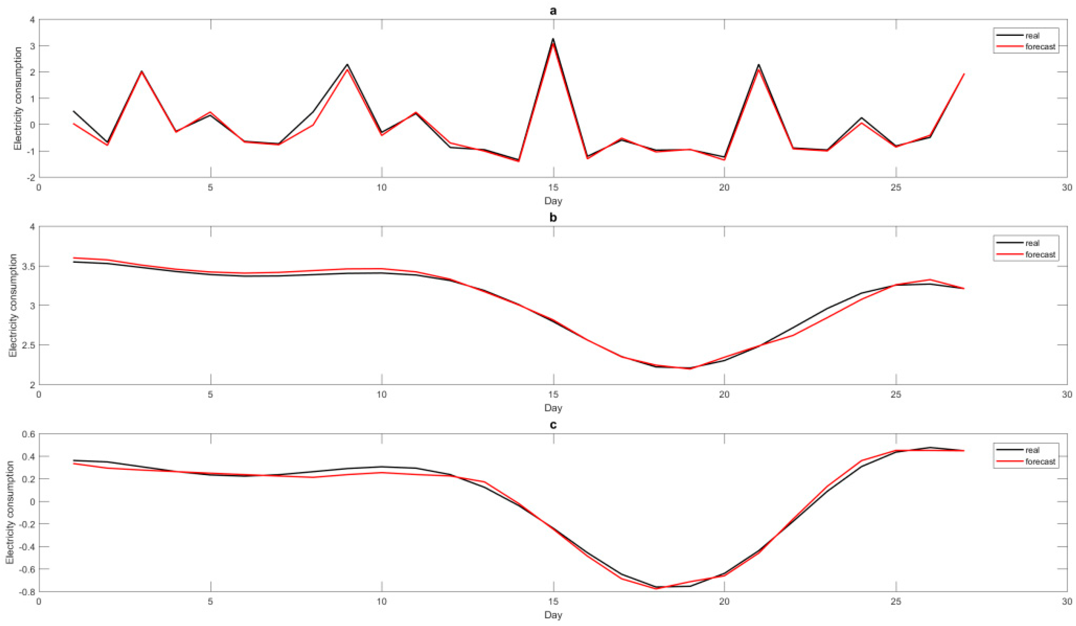
In the dormitory II case, the three items A, B, and C, defined by the six IMFs are also separately modeled by the SVR-QGA model to determine the most appropriate parameter combination of their associated SVR-based models. The appropriate parameter combination for each item for other compared models, including the original SVR model, the SVR-QGA model, the H-EMD-SVR-PSO model [40], are illustrated in

Table 4. The parameters of the EMD-SVR-QGA model and other compared models in the dormitory II case.

Compared Models and Defined Items	Parameter Combination of the SVR Model
	$\mathit{\sigma }$	C	$\mathit{\epsilon }$
The original SVR model	2.80	100.00	0.50
The SVR-QGA model	0.89	37.29	0.17
The H-EMD-SVR-PSO model [40]
Item A: the random term + the middle term	0.18	95.00	0.0011
Item B: the middle term + the trend (residual) term	0.18	96.00	0.0011
Item C: the middle term	0.20	98.00	0.0013
The EMD-SVR-QGA model
Item A: all terms—the trend (residual) term	0.46	3.01	0.0266
Item B: all terms—top two IMFs	0.49	2.02	0.0305
Item C: all terms—top two IMFs—the trend (residual) term	0.47	2.34	0.0567

. The forecasting performances for the three items are demonstrated in Figure 9.

For the dormitory II case, the forecasting results of the original SVR model, the SVR-QGA model [50], the H-EMD-SVR-PSO model [40], and the proposed EMD-SVR-QGA model are shown in Figure 10. It also demonstrates the forecasting curve of the proposed EMD-SVR-QGA model fits better with the actual electricity consumption than other compared models. It also implies that the proposed EMD-SVR-QGA model is qualified to well deal with the fluctuation characteristics of the electricity consumption from this dormitory. Thus, it could contribute to the campus managers providing more insight governance policy for the electricity-saving of the dormitory.

The forecasting performance of these models is listed in

Table 5. Forecasting performance for the EMD-SVR-QGA and other compared models in the dormitory II case.

Compared Models	MAPE	RMSE	MSE	MAE
The original SVR	11.24	0.31	0.10	0.29
The SVR-QGA [50]	7.29	0.58	0.33	0.28
The H-EMD-SVR-PSO [40]	5.35	0.21	0.05	0.17
The EMD-SVR-QGA	4.18	0.16	0.03	0.12

. As the same results in the dormitory I case, the proposed EMD-SVR-QGA model also shows better generalization ability than other models, the original SVR model, the SVR-QGA model [50], and the H-EMD-SVR-PSO model [40] in terms of four employed forecasting accuracy indexes. The forecasting advantages from this kind of EMD-SVR-based model are revealed once again. Different combination types of these decomposed IMFs and the residual term could obtain different forecasting accuracy. It is deserved to look for a suitable IMFs combination approach.

Furthermore, from Table 5, the forecasting results support the same conclusion in Dormitory I case once again: the EMD-SVR-based models able to well deal with this inherent non-linear data pattern by the IMFs and these defined items, A, B, and C. Therefore, the proposed EMD-SVR-QGA model can be a useful forecasting model to deal with the electricity consumption forecasting work of a university dormitory.

For the significance test of the forecasting performance from the proposed EMD-SVR-QGA model, the results of Wilcoxon signed-rank test, based on one-tail-test and is under two significance levels, α = 0.025 and α = 0.05, are shown in

Table 6. Wilcoxon signed-rank test for the dormitory II case.

Compared Models	Wilcoxon Signed-Rank Test
	α = 0.025; W = 107	α = 0.05; W = 119
EMD-SVR-QGA vs. Original SVR	8 *	8 *
EMD-SVR-QGA vs. SVR-QGA	9 *	9 *
EMD-SVR-QGA vs. H-EMD-SVR-PSO	11 *	11 *

Note: * denotes that the EMD-SVR-QGA model significantly outperforms other compared models.

. Obviously, it indicates that the proposed EMD-SVR-QGA model outperforms significantly other compared models.

3.6. Decomposition Results and Forecasting Results for New South Wales (NSW, Australia) Market

Similar to the above two dormitory cases, the electric load data in the New South Wales (NSW, Australia) market is also firstly decomposed by the EMD method into six terms. These six decomposed terms are demonstrated in Figure 11, in which the first IMF and the second IMF are obviously the random terms, the sixth IMF is also obviously the residual term. The three items A, B, and C, defined by the six IMFs are shown in Figure 12.

In the dormitory II case, the three items A, B, and C, defined by the six IMFs are also separately modeled by the SVR-QGA model to determine the most appropriate parameter combination of their associated SVR-based models. The appropriate parameter combination for each item for other compared models, including the original SVR model, the SVR-QGA model, the H-EMD-SVR-PSO model [40], are illustrated in

Table 7. The parameters of the EMD-SVR-QGA model and other compared models in NSW (Australia) case.

Compared Models and Defined Items	Parameter Combination of the SVR Model
	$\mathit{\sigma }$	C	$\mathit{\epsilon }$
The original SVR model	3.16	$1.64\times {10}^3$	0.098
The SVR-QGA model	0.86	$9.49\times {10}^3$	0.750
The H-EMD-SVR-PSO model [40]
Item A: the random term + the middle term	0.14	$1.21\times {10}^4$	0.021
Item B: the middle term + the trend (residual) term	2.27	$1.55\times {10}^4$	0.708
Item C: the middle term	0.41	$6.89\times {10}^3$	0.487
The EMD-SVR-QGA model
Item A: all terms—the trend (residual) term	0.58	$1.35\times {10}^4$	0.905
Item B: all terms—top two IMFs	0.69	$6.44\times {10}^3$	0.454
Item C: all terms—top two IMFs—the trend (residual) term	0.51	$4.34\times {10}^3$	0.049

. The forecasting performances for the three items are demonstrated in Figure 13.

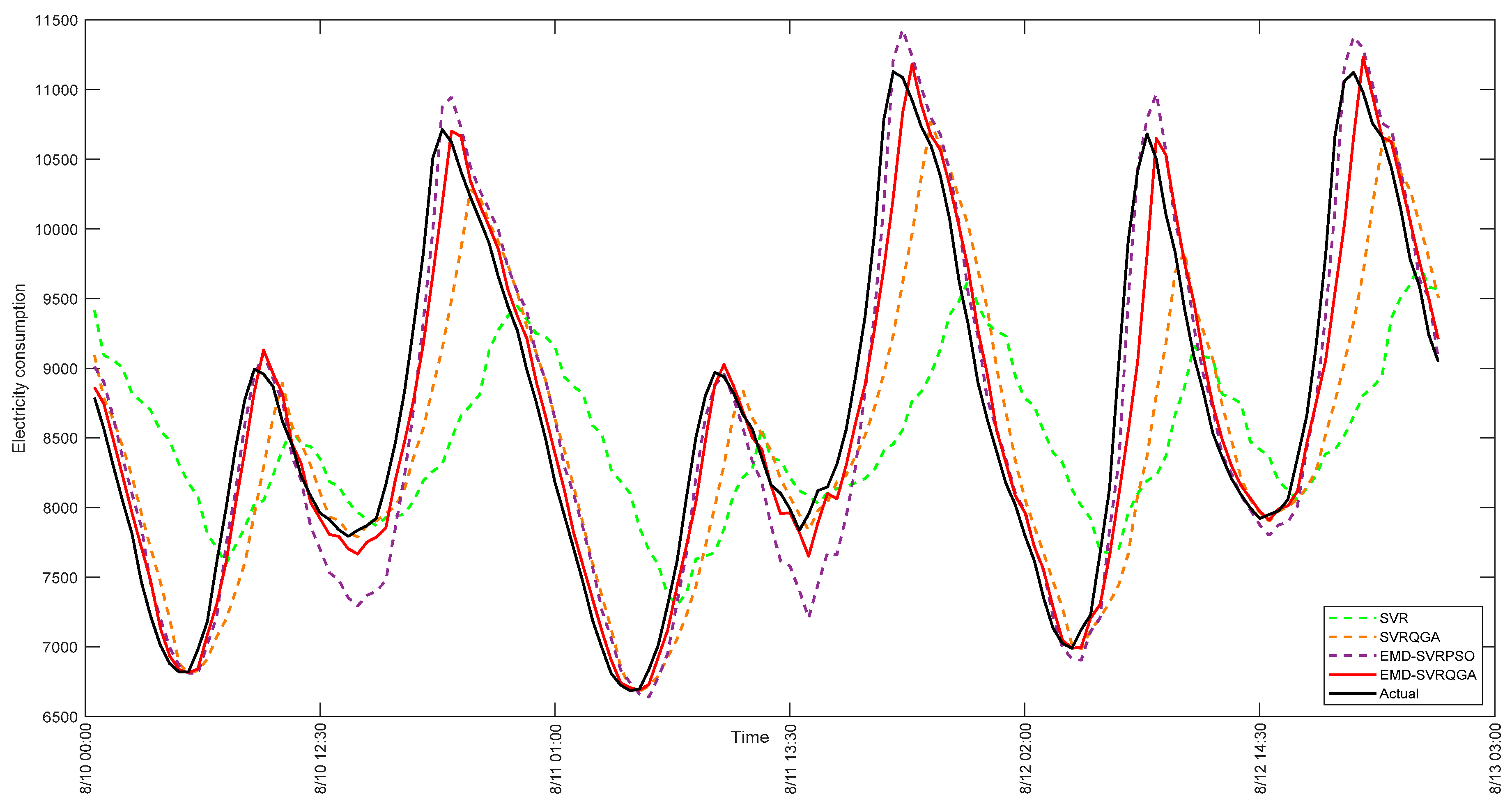
For NSW (Australia) case, the forecasting results of the original SVR model, the SVR-QGA model [50], the H-EMD-SVR-PSO model [40], and the proposed EMD-SVR-QGA model are shown in Figure 14. It also demonstrates the forecasting curve of the proposed EMD-SVR-QGA model fits better with the actual electric load than other compared models. It also implies that the proposed model is qualified to well deal with the fluctuation characteristics of the electric load in real-world applications, such as the NSW market in Australia. Thus, it supports that the proposed model is useful to the campus managers to receive accurate forecasting performance.

The forecasting performance of these models is listed in Table 5. As the same results in dormitory I case, the proposed EMD-SVR-QGA model also shows better generalization ability than other models, the original SVR model, the SVR-QGA model [50], and the H-EMD-SVR-PSO model [40] in terms of four employed forecasting accuracy indexes. It once again reveals the superiority of EMD-SVR-based models.

Furthermore, from

Table 8. Forecasting performance for the EMD-SVR-QGA and other compared models in the NSW (Australia) case.

Compared Models	MAPE	RMSE	MSE	MAE
The original SVR	10.44	$1.15\times {10}^3$	$1.32\times {10}^6$	924.18
The SVR-QGA [50]	5.76	749.07	$5.61\times {10}^5$	531.25
The H-EMD-SVR-PSO [40]	3.24	330.49	$1.09\times {10}^5$	279.55
The EMD-SVR-QGA	2.68	356.01	$1.27\times {10}^5$	245.39

, the forecasting results also support the same conclusion in NSW (Australia) case: the EMD-SVR-based models able to well deal with this inherent non-linear data pattern by the IMFs and these defined items, A, B, and C. Therefore, the proposed EMD-SVR-QGA model is appropriate to be applied to deal with the electricity consumption forecasting work.

For the significance test of the forecasting performance from the proposed EMD-SVR-QGA model, the Wilcoxon signed-rank test is conducted as in the previous two cases, also based on one-tail-test and two significance levels, α = 0.025 and α = 0.05, the tested results are shown in

Table 9. Wilcoxon signed-rank test for NSW (Australia) case.

Compared Models	Wilcoxon Signed-Rank Test
	α = 0.025, p-Value	α = 0.05, p-Value
EMD-SVR-QGA vs. Original SVR	0.0000 **	0.0000 **
EMD-SVR-QGA vs. SVR-QGA	0.0000 **	0.0000 **
EMD-SVR-QGA vs. H-EMD-SVR-PSO	0.0042 **	0.0042 **

Note: ** implies the p-value is lower than α = 0.025.

. Obviously, it indicates that the proposed EMD-SVR-QGA model outperforms significantly other compared models.

3.7. Discussions

As shown in [40], they defined three items (A, B, and C) based on the excellent combination of these different decomposed IMFs, such as the random term, the middle terms, and the residual term. Therefore, a suitable combination of the decomposed IMFs, i.e., how to make good use of these IMFs, could be an interesting issue to help to improve the forecasting accuracy of the proposed model. However, due to the inherent complexity of the employed data set, the decomposition results are varied. For example, in [40], there is only one decomposed IMF with random volatility and the best ones are not, thus, the best combination of these IMFs is demonstrated in [40]. In addition, there may be two or more decomposed IMFs with random volatility, such as in this paper there are two terms with different randomness, therefore, we define different three items, i.e., different combinations of these decomposed IMFs (the proposed EMD-SVR-QGA model). Eventually, we receive more accurate forecasting results than the results using the combination approach (the H-EMD-SVR-PSO model) in [40]. We would like to claim that the superiority of our proposed EMD-SVR-QGA model than the H-EMD-SVR-PSO model.

Therefore, it could be remarked that an effective combination of the decomposed IMFs could provide a clearer cue to understand the complex structure of the employed data set, then, make good use of these IMFs can help to receive more satisfying analysis results, such as forecasting accuracy improvement or classification accuracy enhancement. The exploration of the effective combination of the decomposed IMFs also inspires some interesting future research.

4. Conclusions

This paper proposes a novel EMD-SVR-QGA electricity consumption forecasting model to provide the campus managers with more accurate electricity consumption forecasting from the university dormitory. It is superior in capturing the fluctuation variation of the electricity consumption and reveals its potentials to indicate the daily patterns of the electricity consumption of the dormitory which is useful to take some valuable activities regarding improving electricity consumption habits. The proposed EMD-SVR-QGA model uses different combinations approach of the IMFs decomposed by the EMD method, to well deal with the interaction among those decomposed IMFs and the residual term and the inherent complexity in the electricity consumption data. Furthermore, this paper also applies the QGA to comprehensively search for the appropriate values of the three parameters of an SVR model, then, used the trained SVR-QGA model to forecast the defined items (A, B, and C), separately. It ensures receiving more satisfied forecasting results. Finally, two representative university dormitories’ electricity consumption data sets are used to conduct modeling, the experimental results demonstrate that the proposed model has outperformed significantly other compared models in terms of forecasting accuracy indexes, such as the original SVR model, the SVR-QGA model, and the H-EMD-SVR-PSO model.

The experimental results also indicate the very issues that the different combination of these decomposed IMFs to deal with the inherent nonlinear or other complex interactions among the data set. This issue also asks researchers to carefully study the characteristics of the IMFs, then, determine an effective combination type of these IMFs and the associated SVR-based model. For future research, we will consider hybridizing different intelligent technologies to combine the IMFs, and other useful meta-heuristic algorithm with quantum computing mechanism, to enrich the research contents to receive higher forecasting accuracy.