Using Dynamic Adjusting NGHS-ANN for Predicting the Recidivism Rate of Commuted Prisoners


Abstract
1. Introduction
2. A Review of Five Harmony Search Algorithms
2.1. Harmony Search Algorithm
- Step 1: Determine the problem and initial algorithm parameters, including m, HMCR, PAR, BW, current iteration = 1, and NI.
- Step 2: Generate the initial solutions (harmony memory) randomly and calculate the fitness of each solution.
- Step 3: Generate a trial solution by HMCR, PAR, and BW. The pseudocode of HS algorithm is shown in Algorithm 1.
| Algorithm 1 The Pseudocode of HS |
| 1: 2: 3: 4: 5: 6: 7: 8: 9: 10: 11: 12: 13: 14: 15: |
- Step 4: If the trial solution is better than the worst solution in the HM, replace the worst solution by the trial solution.
- Step 5: If the maximum number of iterations NI is satisfied, return the best solution in the HM; otherwise, the current iteration = + 1 and go back to step 3.
2.2. Improved Harmony Search Algorithm
2.3. Self-Adaptive Global Best Harmony Search Algorithm
- Step 1: Determine the problem and initial algorithm parameters, including m, ,, , , LP, current iteration = 1, and NI.
- Step 2: Generate the initial solutions (harmony memory) randomly and calculate the fitness of each solution.
- Step 3: Generate the algorithm parameters in current iteration , including , , and .
- Step 4: Generate a trial solution by , , and . The pseudocode of SGHS algorithm is shown in Algorithm 2.
| Algorithm 2 The Pseudocode of SGHS [21] |
| 1: 2: 3: 4: 5: 6: 7: 8: 9: 10: 11: 12: 13: 14: 15: |
- Step 5: If the trial solution is better than the worst solution in the HM, replace the worst solution by the trial solution and record the values of HMCR and PAR in current iteration .
- Step 6: Recalculate the and .
- Step 7: If the maximum number of iterations NI is satisfied, return the best solution in the HM; otherwise, the current iteration = + 1 and go back to Step 3.
2.4. Novel Global Harmony Search Algorithm
- Step 1: Determine the problem and initial algorithm parameters, including m, , current iteration = 1, and NI.
- Step 2: Generate the initial solutions (harmony memory) randomly and calculate the fitness of each solution.
- Step 3: Generate a trial solution by . The pseudocode of NGHS algorithm is shown in Algorithm 3.
| Algorithm 3 The Pseudocode of NGHS [18,19,20] |
| 1: 2: 3: 4: 5: 6: 7: 8: 9: 10: 11: 12: |
- Step 4: Replace the worst solution by the trial solution, even if the trial solution is worse than the worst solution.
- Step 5: If the maximum number of iterations NI is satisfied, return the best solution in the HM; otherwise, the current iteration = + 1 and go back to Step 3.
2.5. Dynamic Adjusting Novel Global Harmony Search
3. Experiments and Analysis
3.1. Data Setting
3.2. Computing Environment Settings
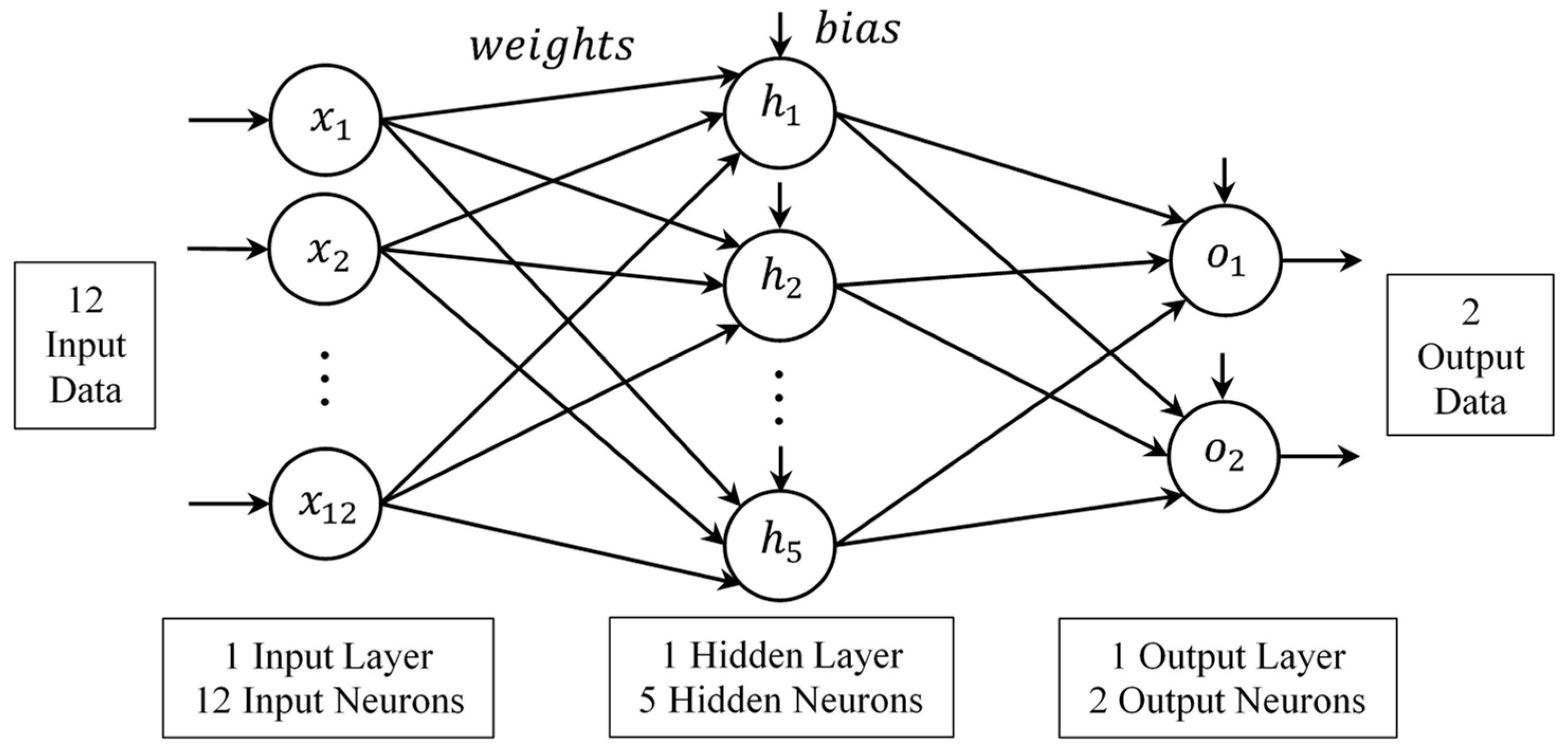
3.3. Experimental Structure and Results of BPN
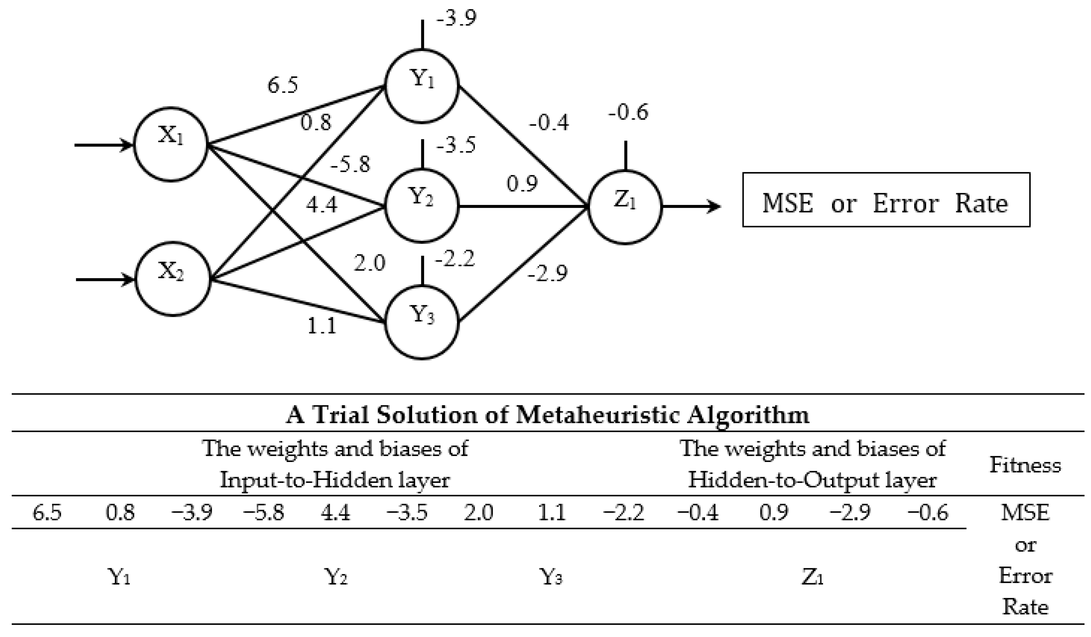
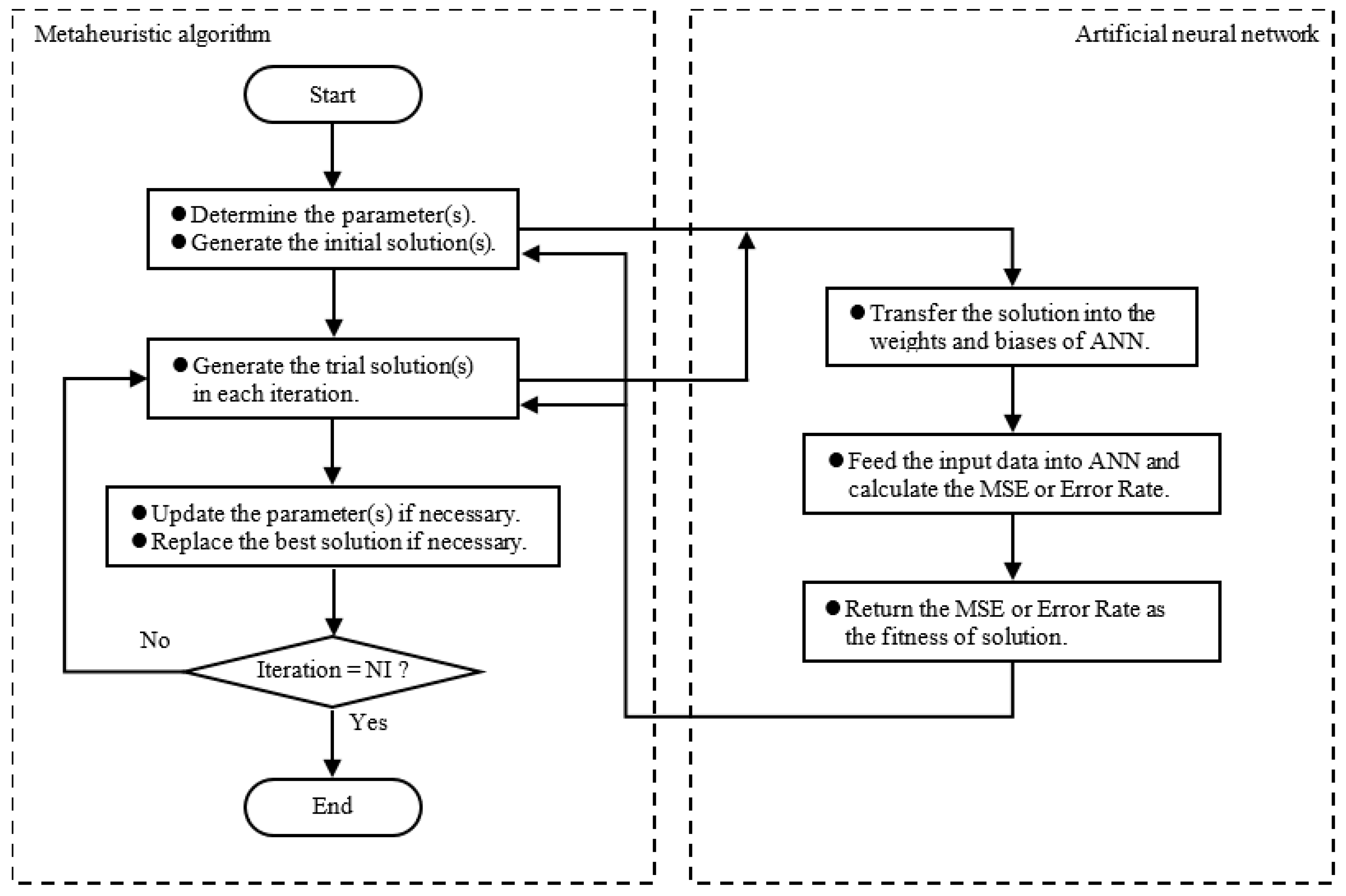
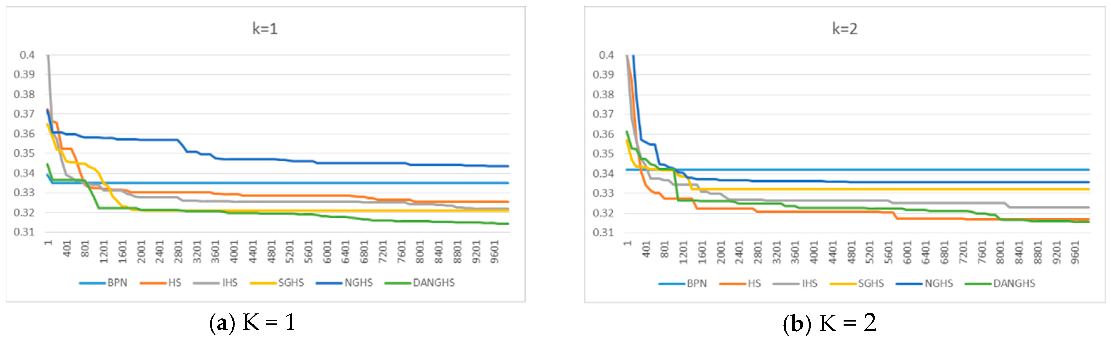
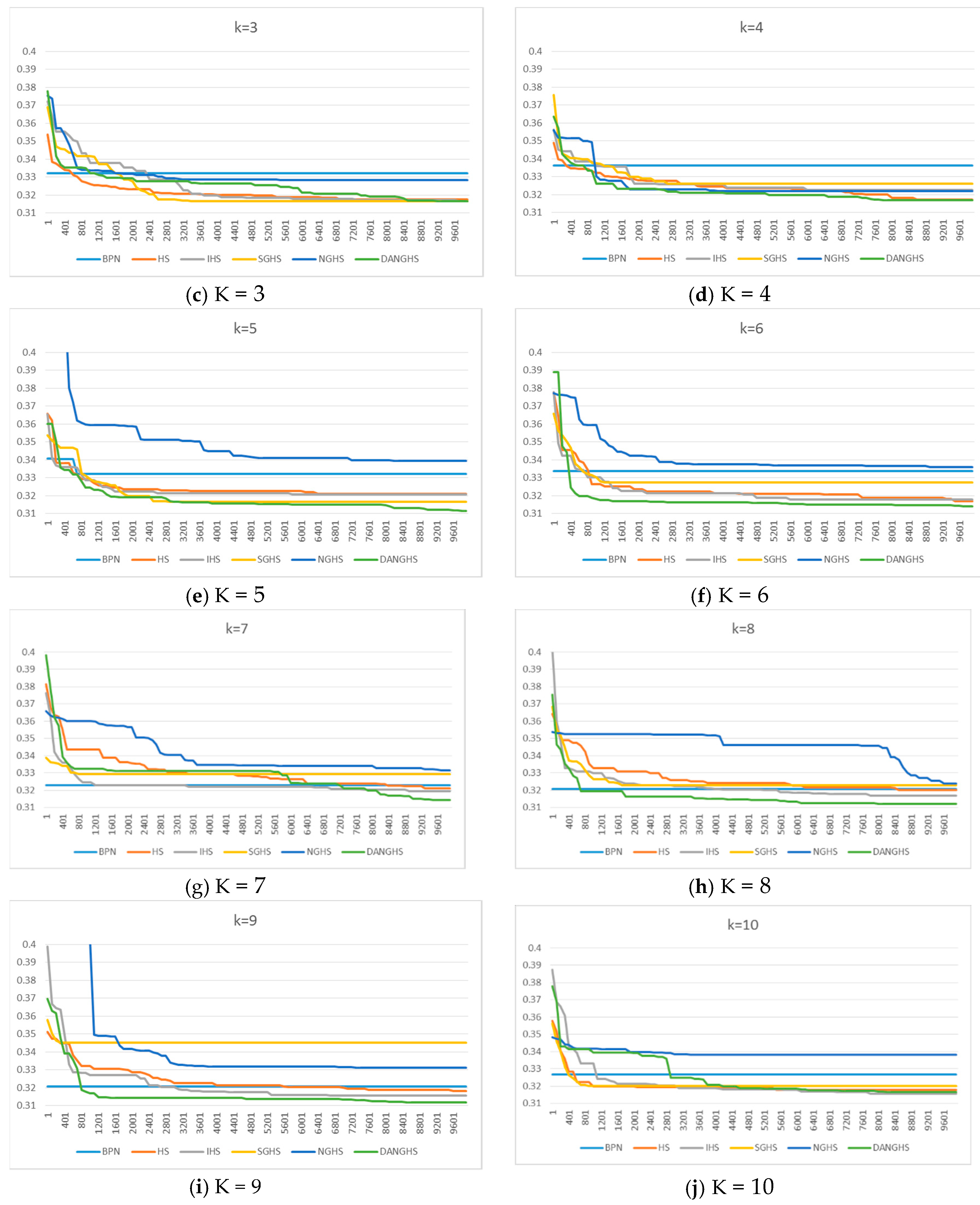
3.4. Experimental Results of the Metaheuristic-ANN Forecasting System
4. Conclusions and Future Research
Author Contributions
Funding
Acknowledgments
Conflicts of Interest
Nomenclature
| ACO | ant colony optimization |
| ANN | artificial neural network |
| AR | association rule |
| BP | backpropagation |
| BPN | backpropagation network |
| BW | bandwidth |
| coefficient of cycle | |
| DANGHS | dynamic adjusting novel global harmony search |
| DE | differential evolution |
| EWR | example-to-weight ratio |
| GA | genetic algorithm |
| HHO | Harris hawks optimization |
| HM | harmony memory |
| HMCR | harmony memory considering rate |
| HS | harmony search |
| IGHS | intelligent global harmony search |
| IHS | improved harmony search |
| current iteration | |
| K | K-fold cross validation |
| LP | learning period |
| m | harmony memory size |
| MCOA | modified coyote optimization algorithm |
| MLP | multilayer perceptron |
| MSE | mean squared error |
| n | total number of experiments |
| NGHS | novel global harmony search |
| NHN | number of hidden neurons |
| NI | maximum number of iterations |
| number of input neurons | |
| number of output neurons | |
| PAR | pitch adjusting rate |
| genetic mutation probability | |
| PSO | particle swarm optimization |
| SGHS | self-adaptive global best harmony search |
| SVM | support vector machine |
| TLBO | teaching learning based optimization |
References
- Carroll, J.S.; Wiener, R.L.; Coates, D.; Galegher, J.; Alibrio, J.J. Evaluation, Diagnosis and Prediction in Parole Decision Making. Law Soc. Rev. 1982, 17, 199–228. [Google Scholar] [CrossRef]
- Williams, F.P.; McShane, M.D.; Dolny, H.M. Predicting Parole Absconders. Prison J. 2000, 80, 24–38. [Google Scholar] [CrossRef]
- MacKenzie, D.L.; Spencer, D.L. The Impact of Formal & Social Controls on the Criminal Activities of Probationers. J. Res. Crime Delinq. 2002, 39, 243–276. [Google Scholar]
- Benda, B.B. Survival Analysis of Criminal Recidivism of Boot Camp Graduates Using Elements From General & Developmental Explanatory Models. Int. J. Offender Ther. 2003, 47, 89–110. [Google Scholar]
- Trulson, C.R.; Marquart, J.W.; Mullings, J.L.; Caeti, T.J. In Between Adolescence and Adulthood: Recidivism Outcomes of a Cohort of State Delinquents. Youth Violence Juv. Justice 2005, 3, 355–387. [Google Scholar] [CrossRef]
- Hwang, J.-I.; Jung, H.-S. Automatic Ship Detection Using the Artificial Neural Network and Support Vector Machine from X-Band Sar Satellite Images. Remote Sens. 2018, 10, 1799. [Google Scholar] [CrossRef]
- Gemitzi, A.; Lakshmi, V. Estimating Groundwater Abstractions at the Aquifer Scale Using GRACE Observations. Geosci. J. 2018, 8, 419. [Google Scholar] [CrossRef]
- Liu, M.-L.; Tien, F.-C. Reclaim wafer defect classification using SVM. In Proceedings of the Asia Pacific Industrial Engineering & Management Systems Conference, Taipei, Taiwan, 7–10 December 2016. [Google Scholar]
- Moodley, R.; Chiclana, F.; Caraffini, F.; Carter, J. A product-centric data mining algorithm for targeted promotions. J. Retail. Consum. Serv. 2019, 3, 101940. [Google Scholar] [CrossRef]
- Tien, F.-C.; Sun, T.-H.; Liu, M.-L. Reclaim Wafer Defect Classification Using Backpropagation Neural Networks. In Proceedings of the International Congress on Recent Development in Engineering and Technology, Kuala Lumpur, Malaysia, 22–24 August 2016. [Google Scholar]
- Tavakoli, S.; Valian, E.; Mohanna, S. Feedforward neural network training using intelligent global harmony search. Evol. Syst. 2012, 3, 125–131. [Google Scholar] [CrossRef]
- Zhang, Q.-J.; Gupta, K.C.; Devabhaktuni, V.K. Artificial Neural Networks for RF and Microwave Design—From Theory to Practice. IEEE Trans. Microw. Theory Thch. 2003, 51, 1339–1350. [Google Scholar] [CrossRef]
- Basheer, I.A.; Hajmeer, M. Artificial neural networks: Fundamentals, computing, design, and application. J. Microbiol. Methods 2000, 43, 3–31. [Google Scholar] [CrossRef]
- Kattan, A.; Abdullah, R. Training of feed-forward neural networks for pattern-classification applications using music inspired algorithm. Int. J. Comput. Sci. Inf. Secur. 2011, 9, 44–57. [Google Scholar]
- Kumaran, J.; Ravi, G. Long-term Sector-wise Electrical Energy Forecasting Using Artificial Neural Network and Biogeography-based Optimization. Electr. Power Compon. Syst. 2015, 43, 1225–1235. [Google Scholar] [CrossRef]
- Göçken, M.; Özçalıcı, M.; Boru, A.; Dosdogru, A.T. Integrating metaheuristics and Artificial Neural Networks for improved stock price prediction. Expert Syst. Appl. 2016, 44, 320–331. [Google Scholar] [CrossRef]
- Chiu, C.-Y.; Shih, P.-C.; Li, X. A Dynamic Adjusting Novel Global Harmony Search for Continuous Optimization Problems. Symmetry 2018, 10, 337. [Google Scholar] [CrossRef]
- Zou, D.; Gao, L.; Li, S.; Wu, J.; Wang, X. A novel global harmony search algorithm for task assignment problem. J. Syst. Softw. 2010, 83, 1678–1688. [Google Scholar] [CrossRef]
- Zou, D.; Gao, L.; Wu, J.; Li, S.; Li, Y. A novel global harmony search algorithm for reliability problems. Comput. Ind. Eng. 2010, 58, 307–316. [Google Scholar] [CrossRef]
- Zou, D.; Gao, L.; Wu, J.; Li, S. Novel global harmony search algorithm for unconstrained problems. Neurocomputing 2010, 73, 3308–3318. [Google Scholar] [CrossRef]
- Pan, Q.K.; Suganthan, P.N.; Tasgetiren, M.F.; Liang, J.J. A self-adaptive global best harmony search algorithm for continuous optimization problems. Appl. Math. Comput. 2010, 216, 830–848. [Google Scholar] [CrossRef]
- Valian, E.; Tavakoli, S.; Mohanna, S. An intelligent global harmony search approach to continuous optimization problems. Appl. Math. Comput. 2014, 232, 670–684. [Google Scholar] [CrossRef]
- Geem, Z.W.; Kim, J.H.; Loganathan, G.V. A new heuristic optimization algorithm: Harmony search. Simulation 2001, 76, 60–68. [Google Scholar] [CrossRef]
- Omran, M.G.H.; Mahdavi, M. Global-best harmony search. Appl. Math. Comput. 2008, 198, 643–656. [Google Scholar] [CrossRef]
- Mahdavi, M.; Fesanghary, M.; Damangir, E. An improved harmony search algorithm for solving optimization problems. Appl. Math. Comput. 2007, 188, 1567–1579. [Google Scholar] [CrossRef]
- Kennedy, J.; Eberhart, R. Particle Swarm Optimization. In Proceedings of the IEEE International Conference on Neural Networks, Perth, Australia, 27 November–1 December 1995. [Google Scholar]
- Eberhart, R.; Kennedy, J. A new optimizer using particle swarm theory. In Proceedings of the Sixth International Symposium on Micro Machine and Human Science, Nagoya, Japan, 4–6 October 1995; pp. 39–43. [Google Scholar]
- Chen, K.H.; Chen, L.F.; Su, C.T. A new particle swarm feature selection method for classification. J. Intell. Inf. Syst. 2014, 42, 507–530. [Google Scholar] [CrossRef]
- Petrović, M.; Vuković, N.; Mitić, M.; Miljković, Z. Integration of process planning and scheduling using chaotic particle swarm optimization algorithm. Expert Syst. Appl. 2016, 64, 569–588. [Google Scholar] [CrossRef]
- Khaled, N.; Hemayed, E.E.; Fayek, M.B. A GA-based approach for epipolar geometry estimation. Int. J. Pattern Recognit. Artif. Intell. 2013, 27, 1355014. [Google Scholar] [CrossRef]
- Metawaa, N.; Hassana, M.K.; Elhoseny, M. Genetic algorithm based model for optimizing bank lending decisions. Expert Syst. Appl. 2017, 80, 75–82. [Google Scholar] [CrossRef]
- Song, S. Design of distributed database systems: An iterative genetic algorithm. J. Intell. Inf. Syst. 2015, 45, 29–59. [Google Scholar] [CrossRef]
- Masters, T. Practical Neural Network Recipes in C++; Academic Press: Boston, MA, USA, 1994; ISBN 9780124790407. [Google Scholar]
- Looney, C.G. Advances in feedforward neural networks: Demystifying knowledge acquiring black boxes. IEEE Trans. Knowl. Data Eng. 1996, 8, 211–226. [Google Scholar] [CrossRef]
- Dowla, F.U.; Rogers, L.L. Solving Problems in Environmental Engineering and Geosciences with Artificial Neural Networks; MIT Press: Cambridge, MA, USA, 1995; ISBN 0262515726. [Google Scholar]
- Haykin, S. Neural Networks: A Comprehensive Foundation; Macmillan: New York, NY, USA, 1994; ISBN 0023527617. [Google Scholar]
- Zupan, J.; Gasteiger, J. Neural Networks for Chemists: An Introduction; VCH: New York, NY, USA, 1993; ISBN 3527286039. [Google Scholar]
- Rao, R.V.; Savsani, V.J.; Vakharia, D.P. Teaching–learning-based optimization: A novel method for constrained mechanical design optimization problems. Comput. Aided Des. 2011, 43, 303–315. [Google Scholar] [CrossRef]
- Li, Z.; Cao, Y.; Dai, L.V.; Yang, X.; Nguyen, T.T. Optimal Power Flow for Transmission Power Networks Using a Novel Metaheuristic Algorithm. Energies 2019, 12, 4310. [Google Scholar] [CrossRef]
- Heidari, A.A.; Mirjalili, S.; Faris, H.; Aljarah, I.; Mafarja, M.; Chen, H. Harris hawks optimization: Algorithm and applications. Future Gener. Comput. Syst. 2019, 97, 849–872. [Google Scholar] [CrossRef]


| Strategy | Description |
|---|---|
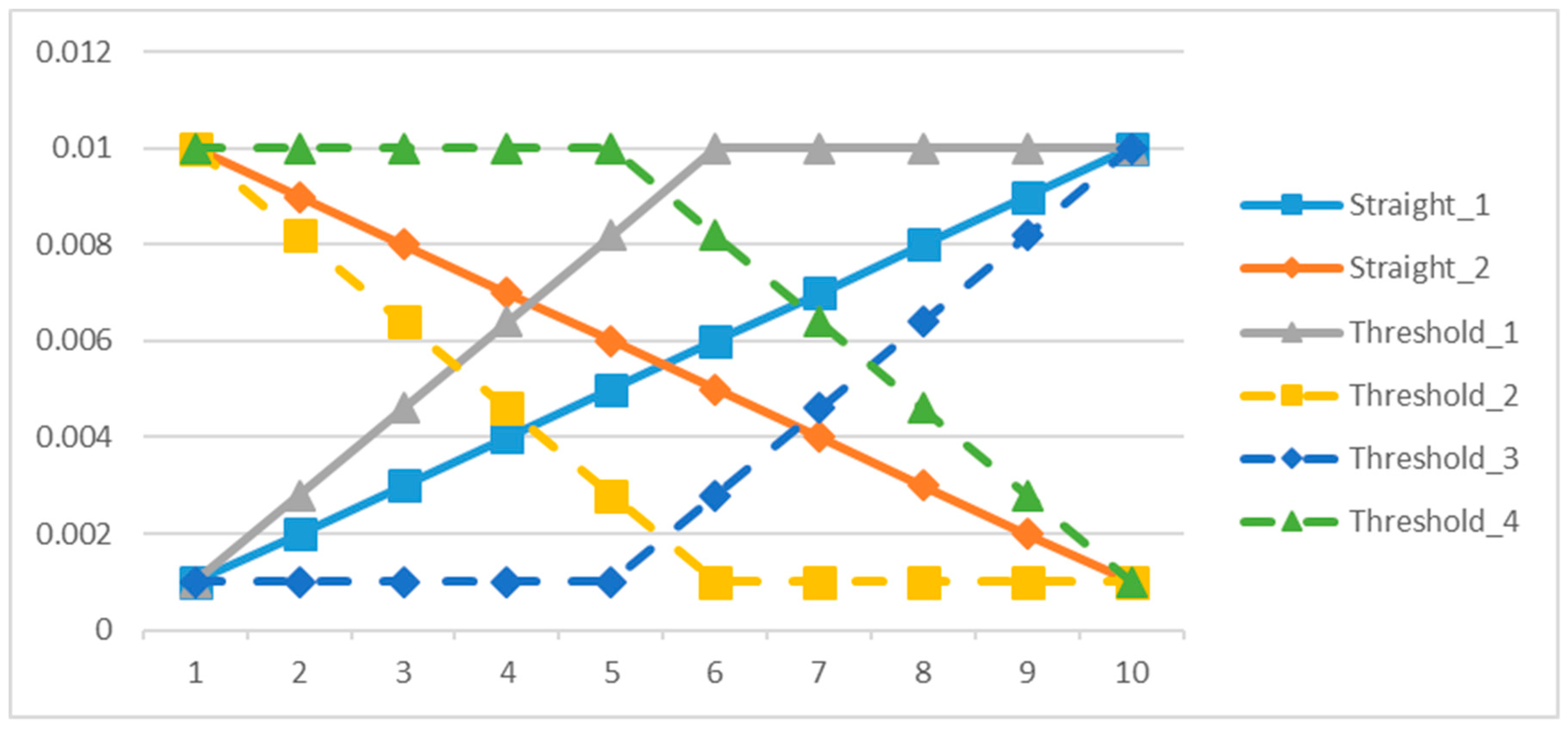
| 1. Straight_1 | Straight linear increasing strategy: |
| 2. Straight_2 | Straight linear decreasing strategy: |
| 3. Threshold_1 | Threshold linear prior increasing strategy: |
| 4. Threshold_2 | Threshold linear prior decreasing strategy: |
| 5. Threshold_3 | Threshold linear posterior increasing strategy: |
| 6. Threshold_4 | Threshold linear posterior decreasing strategy: |
| 7. Exponential_1 | Natural exponential increasing strategy: |
| 8. Exponential_2 | Natural exponential decreasing strategy: |
| 9. Exponential_3 | Exponential increasing strategy with : |
| 10. Exponential_4 | Exponential decreasing strategy with : |
| 11. Exponential_5 | Exponential increasing strategy with : |
| 12. Exponential_6 | Exponential decreasing strategy with : |
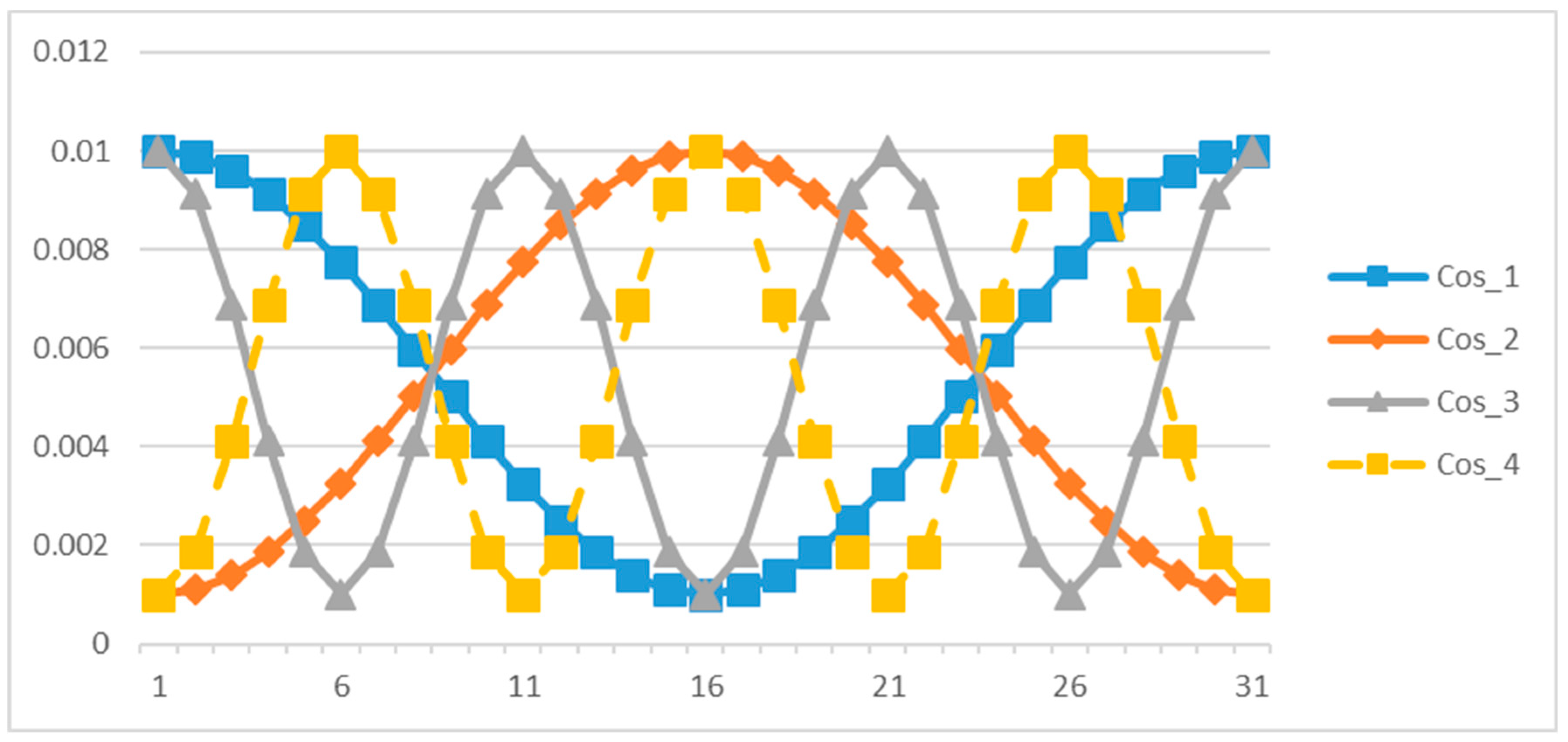
| 13. Cosine_1 | Concave cosine strategy with : |
| 14. Cosine_2 | Convex cosine strategy with : |
| 15. Cosine_3 | Concave cosine strategy with : |
| 16. Cosine_4 | Convex cosine strategy with : |
| Variables | Name | Description |
|---|---|---|
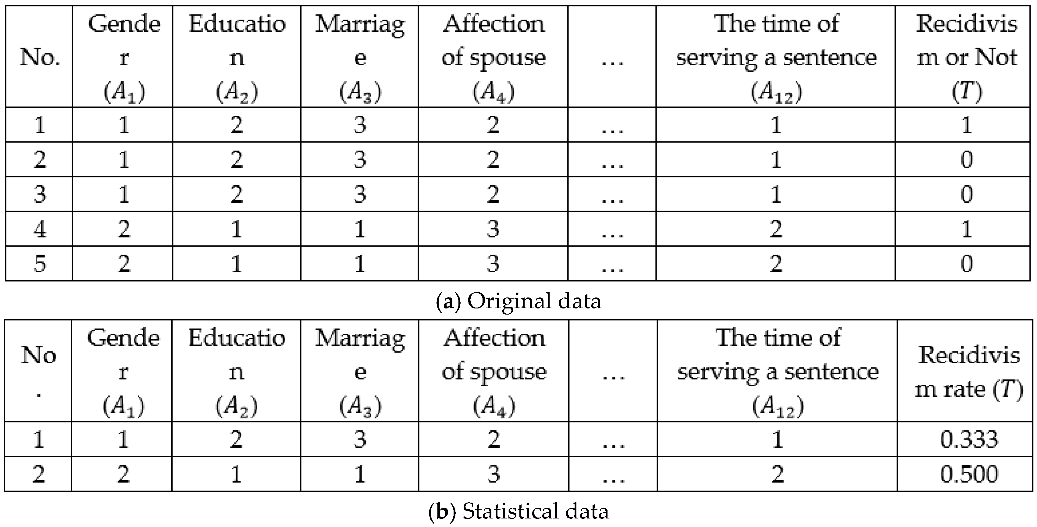
| Input | 1. Gender ) | (1) Male (2) Female |
| 2. Education status ) | (1) Elementary school or illiterate (2) Junior high school (3) Senior high school (4) College or university | |
| 3. Marriage status ) | (1) Unmarried (2) Married (3) Divorced (4) Widowed | |
| 4. Affection of spouse | (1) Unmarried (2) Good (3) Occasional conflict (4) Alienation | |
| 5. Personal or family financial situation | (1) Poverty (2) Barely living (3) Well-to-do (4) Rich | |
| 6. Job satisfaction | (1) Good (2) Normal (3) Not Good (4) Others | |
| 7. Crime | The name of the crime for which they ended up in prison. (1) Crime of embezzlement and dereliction of duty (2) Crime of public danger (3) Crime of forging the seal of documents and securities currency (4) Crime of obstructing weathering (5) Homicide (6) Crime of injury (7) Theft (8) Impairment of freedom (9) Regulations on the control of guns, shells, and knives (10) Drug control regulations (11) Others | |
| 8. Length of criminal experience | The time between the first prosecution and the final prosecution. (1) under 1 year (including) (2) 1 to 5 years (including) (3) 5 to 10 years (including) (4) over 10 years | |
| 9. History of committing a crime | (1) first offense (2) recommit over 5 years (3) recommit within 5 years (including) | |
| 10. The age of going to jail | (1) 19 years old (2) 20–29 years old (3) 30–39 years old (4) 40–49 years old (5) 50–59 years old (6) 60 years old | |
| 11. Total amount of going to jail ) | The cumulative number of going to jail. | |
| 12. The time of serving a sentence | The total days between the imprisonment execution and the release. (1) 180 days (2) 181–365 days (1 year) (3) 366–1095 days (3 years) (4) 1096–1825 days (5 years) (5) 1826 days | |
| Output (original) | Recidivism () | (1) No (2) Yes |
| Output (statistical) | Recidivism rate () | (1) Low (2) High |
| Training | Validation | Testing | |||||||
|---|---|---|---|---|---|---|---|---|---|
| LR | 0.1 | 0.2 | 0.3 | 0.1 | 0.2 | 0.3 | 0.1 | 0.2 | 0.3 |
| MT | 0.9 | 0.8 | 0.7 | 0.9 | 0.8 | 0.7 | 0.9 | 0.8 | 0.7 |
| K = 1 | 3.37 × 10⁻¹ | 3.42 × 10⁻¹ | 3.48 × 10⁻¹ | 3.59 × 10⁻¹ | 3.60 × 10⁻¹ | 3.63 × 10⁻¹ | 3.61 × 10⁻¹ | 3.65 × 10⁻¹ | 3.70 × 10⁻¹ |
| K = 2 | 3.34 × 10⁻¹ | 3.36 × 10⁻¹ | 3.39 × 10⁻¹ | 3.58 × 10⁻¹ | 3.62 × 10⁻¹ | 3.63 × 10⁻¹ | 3.57 × 10⁻¹ | 3.63 × 10⁻¹ | 3.63 × 10⁻¹ |
| K = 3 | 3.31 × 10⁻¹ | 3.38 × 10⁻¹ | 3.46 × 10⁻¹ | 3.57 × 10⁻¹ | 3.59 × 10⁻¹ | 3.64 × 10⁻¹ | 3.61 × 10⁻¹ | 3.62 × 10⁻¹ | 3.69 × 10⁻¹ |
| K = 4 | 3.39 × 10⁻¹ | 3.46 × 10⁻¹ | 3.47 × 10⁻¹ | 3.58 × 10⁻¹ | 3.60 × 10⁻¹ | 3.64 × 10⁻¹ | 3.58 × 10⁻¹ | 3.65 × 10⁻¹ | 3.67 × 10⁻¹ |
| K = 5 | 3.40 × 10⁻¹ | 3.44 × 10⁻¹ | 3.53 × 10⁻¹ | 3.61 × 10⁻¹ | 3.64 × 10⁻¹ | 3.69 × 10⁻¹ | 3.63 × 10⁻¹ | 3.65 × 10⁻¹ | 3.72 × 10⁻¹ |
| K = 6 | 3.20 × 10⁻¹ | 3.27 × 10⁻¹ | 3.28 × 10⁻¹ | 3.53 × 10⁻¹ | 3.56 × 10⁻¹ | 3.57 × 10⁻¹ | 3.50 × 10⁻¹ | 3.49 × 10⁻¹ | 3.50 × 10⁻¹ |
| K = 7 | 3.12 × 10⁻¹ | 3.17 × 10⁻¹ | 3.19 × 10⁻¹ | 3.41 × 10⁻¹ | 3.49 × 10⁻¹ | 3.53 × 10⁻¹ | 3.47 × 10⁻¹ | 3.47 × 10⁻¹ | 3.49 × 10⁻¹ |
| K = 8 | 3.13 × 10⁻¹ | 3.15 × 10⁻¹ | 3.20 × 10⁻¹ | 3.43 × 10⁻¹ | 3.43 × 10⁻¹ | 3.46 × 10⁻¹ | 3.47 × 10⁻¹ | 3.48 × 10⁻¹ | 3.47 × 10⁻¹ |
| K = 9 | 3.10 × 10⁻¹ | 3.15 × 10⁻¹ | 3.14 × 10⁻¹ | 3.47 × 10⁻¹ | 3.55 × 10⁻¹ | 3.56 × 10⁻¹ | 3.48 × 10⁻¹ | 3.50 × 10⁻¹ | 3.57 × 10⁻¹ |
| K = 10 | 3.13 × 10⁻¹ | 3.16 × 10⁻¹ | 3.16 × 10⁻¹ | 3.51 × 10⁻¹ | 3.62 × 10⁻¹ | 3.62 × 10⁻¹ | 3.24 × 10⁻¹ | 3.32 × 10⁻¹ | 3.36 × 10⁻¹ |
| Mean | 3.25 × 10⁻¹ | 3.29 × 10⁻¹ | 3.33 × 10⁻¹ | 3.53 × 10⁻¹ | 3.57 × 10⁻¹ | 3.60 × 10⁻¹ | 3.52 × 10⁻¹ | 3.55 × 10⁻¹ | 3.58 × 10⁻¹ |
| Std | 1.53 × 10⁻⁴ | 1.69 × 10⁻⁴ | 2.34 × 10⁻⁴ | 5.15 × 10⁻⁵ | 4.16 × 10⁻⁵ | 4.51 × 10⁻⁵ | 1.32× 10⁻⁴ | 1.23 × 10⁻⁴ | 1.47 × 10⁻⁴ |
| p-value | - | 6.48 × 10⁻⁶ | 6.37 × 10⁻⁵ | - | 2.76 × 10⁻³ | 3.29 × 10⁻⁵ | - | 4.73 × 10⁻³ | 4.95 × 10⁻⁴ |
| Algorithm | m 1 | HMCR 2 | PAR 3 | BW 4 | LP 5 | NI 7 | n 8 | |
|---|---|---|---|---|---|---|---|---|
| HS | 5 | 0.9 | 0.3 | 0.01 | – | – | 10,000 | 30 |
| IHS | 5 | 0.9 | – | – | 10,000 | 30 | ||
| SGHS | 5 | 100 | – | 10,000 | 30 | |||
| NGHS | 5 | – | – | – | – | 0.05 | 10,000 | 30 |
| DANGHS | 5 | – | – | – | – | 10,000 | 30 |
| Adjustment Strategy | K = 1 | K = 2 | K = 3 | K = 4 | K = 5 | K = 6 | K = 7 | K = 8 | K = 9 | K = 10 | Mean | Std | p-Value |
|---|---|---|---|---|---|---|---|---|---|---|---|---|---|
| Straight_1 | 3.2224 × 10⁻¹ | 3.2045 × 10⁻¹ | 3.1967 × 10⁻¹ | 3.1983 × 10⁻¹ | 3.2095 × 10⁻¹ | 3.2206 × 10⁻¹ | 3.2002 × 10⁻¹ | 3.1880 × 10⁻¹ | 3.1785 × 10⁻¹ | 3.1812 × 10⁻¹ | 3.2000 × 10⁻¹ | 2.2328 × 10⁻⁶ | 0.0000 |
| Straight_2 | 3.1329 × 10⁻¹ | 3.1226 × 10⁻¹ | 3.1410 × 10⁻¹ | 3.1216 × 10⁻¹ | 3.1125 × 10⁻¹ | 3.1393 × 10⁻¹ | 3.1247 × 10⁻¹ | 3.1013 × 10⁻¹ | 3.0923 × 10⁻¹ | 3.0959 × 10⁻¹ | 3.1184 × 10⁻¹ | 3.0458 × 10⁻⁶ | 0.0803 |
| Threshold_1 | 3.2302 × 10⁻¹ | 3.2086 × 10⁻¹ | 3.2260 × 10⁻¹ | 3.2105 × 10⁻¹ | 3.2164 × 10⁻¹ | 3.2066 × 10⁻¹ | 3.2231 × 10⁻¹ | 3.1788 × 10⁻¹ | 3.2048 × 10⁻¹ | 3.1847 × 10⁻¹ | 3.2090 × 10⁻¹ | 2.7978 × 10⁻⁶ | 0.0000 |
| Threshold_2 | 3.1543 × 10⁻¹ | 3.1442 × 10⁻¹ | 3.1369 × 10⁻¹ | 3.1388 × 10⁻¹ | 3.1590 × 10⁻¹ | 3.1322 × 10⁻¹ | 3.1462 × 10⁻¹ | 3.1297 × 10⁻¹ | 3.1091 × 10⁻¹ | 3.1115 × 10⁻¹ | 3.1362 × 10⁻¹ | 2.6869 × 10⁻⁶ | 0.0000 |
| Threshold_3 | 3.2455 × 10⁻¹ | 3.2504 × 10⁻¹ | 3.2758 × 10⁻¹ | 3.2493 × 10⁻¹ | 3.2344 × 10⁻¹ | 3.2536 × 10⁻¹ | 3.2393 × 10⁻¹ | 3.2399 × 10⁻¹ | 3.2304 × 10⁻¹ | 3.2106 × 10⁻¹ | 3.2429 × 10⁻¹ | 2.8818 × 10⁻⁶ | 0.0000 |
| Threshold_4 | 3.1190 × 10⁻¹ | 3.1194 × 10⁻¹ | 3.1240 × 10⁻¹ | 3.1248 × 10⁻¹ | 3.1201 × 10⁻¹ | 3.1131 × 10⁻¹ | 3.1193 × 10⁻¹ | 3.0977 × 10⁻¹ | 3.0985 × 10⁻¹ | 3.0960 × 10⁻¹ | 3.1132 × 10⁻¹ | 1.2896 × 10⁻⁶ | - |
| Exponential_1 | 3.2783 × 10⁻¹ | 3.2590 × 10⁻¹ | 3.2545 × 10⁻¹ | 3.2444 × 10⁻¹ | 3.2537 × 10⁻¹ | 3.2610 × 10⁻¹ | 3.2571 × 10⁻¹ | 3.2314 × 10⁻¹ | 3.2227 × 10⁻¹ | 3.2314 × 10⁻¹ | 3.2493 × 10⁻¹ | 2.8363 × 10⁻⁶ | 0.0000 |
| Exponential_2 | 3.1545 × 10⁻¹ | 3.1680 × 10⁻¹ | 3.1691 × 10⁻¹ | 3.1674 × 10⁻¹ | 3.1451 × 10⁻¹ | 3.1726 × 10⁻¹ | 3.1569 × 10⁻¹ | 3.1341 × 10⁻¹ | 3.1087 × 10⁻¹ | 3.1194 × 10⁻¹ | 3.1496 × 10⁻¹ | 4.9831 × 10⁻⁶ | 0.0000 |
| Exponential_3 | 3.2508 × 10⁻¹ | 3.2614 × 10⁻¹ | 3.2427 × 10⁻¹ | 3.2428 × 10⁻¹ | 3.2498 × 10⁻¹ | 3.2655 × 10⁻¹ | 3.2378 × 10⁻¹ | 3.2595 × 10⁻¹ | 3.2178 × 10⁻¹ | 3.2161 × 10⁻¹ | 3.2444 × 10⁻¹ | 2.8763 × 10⁻⁶ | 0.0000 |
| Exponential_4 | 3.1474 × 10⁻¹ | 3.1436 × 10⁻¹ | 3.1577 × 10⁻¹ | 3.1473 × 10⁻¹ | 3.1433 × 10⁻¹ | 3.1472 × 10⁻¹ | 3.1518 × 10⁻¹ | 3.1390 × 10⁻¹ | 3.1197 × 10⁻¹ | 3.1098 × 10⁻¹ | 3.1407 × 10⁻¹ | 2.1770 × 10⁻⁶ | 0.0000 |
| Exponential_5 | 3.2805 × 10⁻¹ | 3.2650 × 10⁻¹ | 3.2835 × 10⁻¹ | 3.2599 × 10⁻¹ | 3.2738 × 10⁻¹ | 3.2415 × 10⁻¹ | 3.2708 × 10⁻¹ | 3.2527 × 10⁻¹ | 3.2416 × 10⁻¹ | 3.2602 × 10⁻¹ | 3.2629 × 10⁻¹ | 2.1714 × 10⁻⁶ | 0.0000 |
| Exponential_6 | 3.1707 × 10⁻¹ | 3.1588 × 10⁻¹ | 3.1800 × 10⁻¹ | 3.1653 × 10⁻¹ | 3.1622 × 10⁻¹ | 3.1787 × 10⁻¹ | 3.1793 × 10⁻¹ | 3.1428 × 10⁻¹ | 3.1315 × 10⁻¹ | 3.1343 × 10⁻¹ | 3.1604 × 10⁻¹ | 3.3797 × 10⁻⁶ | 0.0000 |
| Cosine_1 | 3.1494 × 10⁻¹ | 3.1517 × 10⁻¹ | 3.1399 × 10⁻¹ | 3.1446 × 10⁻¹ | 3.1385 × 10⁻¹ | 3.1344 × 10⁻¹ | 3.1407 × 10⁻¹ | 3.1205 × 10⁻¹ | 3.1102 × 10⁻¹ | 3.0983 × 10⁻¹ | 3.1328 × 10⁻¹ | 3.0754 × 10⁻⁶ | 0.0000 |
| Cosine_2 | 3.1846 × 10⁻¹ | 3.1709 × 10⁻¹ | 3.1760 × 10⁻¹ | 3.1545 × 10⁻¹ | 3.1765 × 10⁻¹ | 3.1624 × 10⁻¹ | 3.1913 × 10⁻¹ | 3.1698 × 10⁻¹ | 3.1509 × 10⁻¹ | 3.1466 × 10⁻¹ | 3.1683 × 10⁻¹ | 2.1483 × 10⁻⁶ | 0.0000 |
| Cosine_3 | 3.1599 × 10⁻¹ | 3.1567 × 10⁻¹ | 3.1668 × 10⁻¹ | 3.1618 × 10⁻¹ | 3.1529 × 10⁻¹ | 3.1675 × 10⁻¹ | 3.1805 × 10⁻¹ | 3.1431 × 10⁻¹ | 3.1281 × 10⁻¹ | 3.1388 × 10⁻¹ | 3.1556 × 10⁻¹ | 2.3853 × 10⁻⁶ | 0.0000 |
| Cosine_4 | 3.1636 × 10⁻¹ | 3.1981 × 10⁻¹ | 3.1802 × 10⁻¹ | 3.1638 × 10⁻¹ | 3.1922 × 10⁻¹ | 3.1721 × 10⁻¹ | 3.1902 × 10⁻¹ | 3.1489 × 10⁻¹ | 3.1464 × 10⁻¹ | 3.1321 × 10⁻¹ | 3.1688 × 10⁻¹ | 4.7776 × 10⁻⁶ | 0.0000 |
| Adjustment Strategy | K = 1 | K = 2 | K = 3 | K = 4 | K = 5 | K = 6 | K = 7 | K = 8 | K = 9 | K = 10 | Mean | Std | p-Value |
|---|---|---|---|---|---|---|---|---|---|---|---|---|---|
| Straight_1 | 3.5066 × 10⁻¹ | 3.5110 × 10⁻¹ | 3.5071 × 10⁻¹ | 3.4900 × 10⁻¹ | 3.5398 × 10⁻¹ | 3.5081 × 10⁻¹ | 3.5212 × 10⁻¹ | 3.5622 × 10⁻¹ | 3.5442 × 10⁻¹ | 3.3011 × 10⁻¹ | 3.4991 × 10⁻¹ | 5.3088 × 10⁻⁵ | 0.0000 |
| Straight_2 | 3.4168 × 10⁻¹ | 3.4021 × 10⁻¹ | 3.4280 × 10⁻¹ | 3.3963 × 10⁻¹ | 3.4012 × 10⁻¹ | 3.4187 × 10⁻¹ | 3.4139 × 10⁻¹ | 3.4207 × 10⁻¹ | 3.4041 × 10⁻¹ | 3.2265 × 10⁻¹ | 3.3928 × 10⁻¹ | 3.5199 × 10⁻⁵ | 0.2606 |
| Threshold_1 | 3.5188 × 10⁻¹ | 3.4963 × 10⁻¹ | 3.5129 × 10⁻¹ | 3.4968 × 10⁻¹ | 3.5242 × 10⁻¹ | 3.4788 × 10⁻¹ | 3.5266 × 10⁻¹ | 3.5076 × 10⁻¹ | 3.5149 × 10⁻¹ | 3.3353 × 10⁻¹ | 3.4912 × 10⁻¹ | 3.2137 × 10⁻⁵ | 0.0000 |
| Threshold_2 | 3.4563 × 10⁻¹ | 3.4251 × 10⁻¹ | 3.4207 × 10⁻¹ | 3.4412 × 10⁻¹ | 3.4490 × 10⁻¹ | 3.4095 × 10⁻¹ | 3.4456 × 10⁻¹ | 3.4797 × 10⁻¹ | 3.4602 × 10⁻¹ | 3.2445 × 10⁻¹ | 3.4232 × 10⁻¹ | 4.3649 × 10⁻⁵ | 0.0000 |
| Threshold_3 | 3.5368 × 10⁻¹ | 3.5051 × 10⁻¹ | 3.5876 × 10⁻¹ | 3.5549 × 10⁻¹ | 3.5183 × 10⁻¹ | 3.5188 × 10⁻¹ | 3.5432 × 10⁻¹ | 3.5539 × 10⁻¹ | 3.5471 × 10⁻¹ | 3.2918 × 10⁻¹ | 3.5158 × 10⁻¹ | 6.7327 × 10⁻⁵ | 0.0000 |
| Threshold_4 | 3.3934 × 10⁻¹ | 3.4261 × 10⁻¹ | 3.4036 × 10⁻¹ | 3.4222 × 10⁻¹ | 3.4295 × 10⁻¹ | 3.3953 × 10⁻¹ | 3.4139 × 10⁻¹ | 3.4031 × 10⁻¹ | 3.4017 × 10⁻¹ | 3.1889 × 10⁻¹ | 3.3878 × 10⁻¹ | 5.0441 × 10⁻⁵ | - |
| Exponential_1 | 3.6271 × 10⁻¹ | 3.5754 × 10⁻¹ | 3.5549 × 10⁻¹ | 3.5520 × 10⁻¹ | 3.5925 × 10⁻¹ | 3.5408 × 10⁻¹ | 3.5735 × 10⁻¹ | 3.5573 × 10⁻¹ | 3.5422 × 10⁻¹ | 3.3709 × 10⁻¹ | 3.5487 × 10⁻¹ | 4.5814 × 10⁻⁵ | 0.0000 |
| Exponential_2 | 3.4563 × 10⁻¹ | 3.4461 × 10⁻¹ | 3.4592 × 10⁻¹ | 3.4470 × 10⁻¹ | 3.4231 × 10⁻¹ | 3.4763 × 10⁻¹ | 3.4841 × 10⁻¹ | 3.4739 × 10⁻¹ | 3.4563 × 10⁻¹ | 3.2099 × 10⁻¹ | 3.4332 × 10⁻¹ | 6.4665 × 10⁻⁵ | 0.0000 |
| Exponential_3 | 3.5583 × 10⁻¹ | 3.5798 × 10⁻¹ | 3.5647 × 10⁻¹ | 3.5295 × 10⁻¹ | 3.5739 × 10⁻¹ | 3.5881 × 10⁻¹ | 3.5686 × 10⁻¹ | 3.6232 × 10⁻¹ | 3.5364 × 10⁻¹ | 3.3621 × 10⁻¹ | 3.5485 × 10⁻¹ | 4.9757 × 10⁻⁵ | 0.0000 |
| Exponential_4 | 3.4256 × 10⁻¹ | 3.4505 × 10⁻¹ | 3.4705 × 10⁻¹ | 3.4592 × 10⁻¹ | 3.4397 × 10⁻¹ | 3.4290 × 10⁻¹ | 3.4241 × 10⁻¹ | 3.4959 × 10⁻¹ | 3.4275 × 10⁻¹ | 3.2113 × 10⁻¹ | 3.4233 × 10⁻¹ | 6.0866 × 10⁻⁵ | 0.0000 |
| Exponential_5 | 3.5939 × 10⁻¹ | 3.5461 × 10⁻¹ | 3.5691 × 10⁻¹ | 3.5598 × 10⁻¹ | 3.5588 × 10⁻¹ | 3.5500 × 10⁻¹ | 3.5608 × 10⁻¹ | 3.6105 × 10⁻¹ | 3.5588 × 10⁻¹ | 3.3821 × 10⁻¹ | 3.5490 × 10⁻¹ | 3.8344 × 10⁻⁵ | 0.0000 |
| Exponential_6 | 3.4778 × 10⁻¹ | 3.4470 × 10⁻¹ | 3.4778 × 10⁻¹ | 3.4758 × 10⁻¹ | 3.4456 × 10⁻¹ | 3.4534 × 10⁻¹ | 3.4905 × 10⁻¹ | 3.4568 × 10⁻¹ | 3.4871 × 10⁻¹ | 3.2650 × 10⁻¹ | 3.4477 × 10⁻¹ | 4.3867 × 10⁻⁵ | 0.0000 |
| Cosine_1 | 3.4412 × 10⁻¹ | 3.4422 × 10⁻¹ | 3.4168 × 10⁻¹ | 3.4451 × 10⁻¹ | 3.4505 × 10⁻¹ | 3.4114 × 10⁻¹ | 3.4363 × 10⁻¹ | 3.4427 × 10⁻¹ | 3.4441 × 10⁻¹ | 3.2020 × 10⁻¹ | 3.4132 × 10⁻¹ | 5.6652 × 10⁻⁵ | 0.0000 |
| Cosine_2 | 3.4744 × 10⁻¹ | 3.4910 × 10⁻¹ | 3.4578 × 10⁻¹ | 3.4231 × 10⁻¹ | 3.4549 × 10⁻¹ | 3.4295 × 10⁻¹ | 3.4822 × 10⁻¹ | 3.5232 × 10⁻¹ | 3.4622 × 10⁻¹ | 3.2552 × 10⁻¹ | 3.4453 × 10⁻¹ | 5.3057 × 10⁻⁵ | 0.0000 |
| Cosine_3 | 3.4490 × 10⁻¹ | 3.4578 × 10⁻¹ | 3.4685 × 10⁻¹ | 3.4900 × 10⁻¹ | 3.4563 × 10⁻¹ | 3.4661 × 10⁻¹ | 3.5110 × 10⁻¹ | 3.4505 × 10⁻¹ | 3.4632 × 10⁻¹ | 3.2733 × 10⁻¹ | 3.4486 × 10⁻¹ | 4.1550 × 10⁻⁵ | 0.0000 |
| Cosine_4 | 3.4568 × 10⁻¹ | 3.5100 × 10⁻¹ | 3.4939 × 10⁻¹ | 3.4671 × 10⁻¹ | 3.4680 × 10⁻¹ | 3.4754 × 10⁻¹ | 3.4993 × 10⁻¹ | 3.4822 × 10⁻¹ | 3.4685 × 10⁻¹ | 3.2299 × 10⁻¹ | 3.4551 × 10⁻¹ | 6.5375 × 10⁻⁵ | 0.0000 |
| Forecasting System | K = 1 | K = 2 | K = 3 | K = 4 | K = 5 | K = 6 | K = 7 | K = 8 | K = 9 | K = 10 | Mean | Std | p-Value |
|---|---|---|---|---|---|---|---|---|---|---|---|---|---|
| BPN | 3.4310 × 10⁻¹ | 3.4085 × 10⁻¹ | 3.3810 × 10⁻¹ | 3.4446 × 10⁻¹ | 3.4561 × 10⁻¹ | 3.2902 × 10⁻¹ | 3.2040 × 10⁻¹ | 3.2120 × 10⁻¹ | 3.2023 × 10⁻¹ | 3.2342 × 10⁻¹ | 3.3264 × 10⁻¹ | 1.0787 × 10⁻² | 0.0000 |
| HS-ANN | 3.1379 × 10⁻¹ | 3.1470 × 10⁻¹ | 3.1366 × 10⁻¹ | 3.1551 × 10⁻¹ | 3.1467 × 10⁻¹ | 3.1442 × 10⁻¹ | 3.1317 × 10⁻¹ | 3.1245 × 10⁻¹ | 3.1218 × 10⁻¹ | 3.1114 × 10⁻¹ | 3.1357 × 10⁻¹ | 1.3453 × 10⁻³ | 0.0000 |
| IHS-ANN | 3.1465 × 10⁻¹ | 3.1377 × 10⁻¹ | 3.1412 × 10⁻¹ | 3.1447 × 10⁻¹ | 3.1356 × 10⁻¹ | 3.1419 × 10⁻¹ | 3.1332 × 10⁻¹ | 3.1191 × 10⁻¹ | 3.1049 × 10⁻¹ | 3.1097 × 10⁻¹ | 3.1315 × 10⁻¹ | 1.4893 × 10⁻³ | 0.0000 |
| SGHS-ANN | 3.4227 × 10⁻¹ | 3.4464 × 10⁻¹ | 3.4309 × 10⁻¹ | 3.4375 × 10⁻¹ | 3.4198 × 10⁻¹ | 3.4377 × 10⁻¹ | 3.4365 × 10⁻¹ | 3.4092 × 10⁻¹ | 3.4061 × 10⁻¹ | 3.4048 × 10⁻¹ | 3.4252 × 10⁻¹ | 1.4864 × 10⁻³ | 0.0000 |
| NGHS-ANN | 3.1622 × 10⁻¹ | 3.1682 × 10⁻¹ | 3.1586 × 10⁻¹ | 3.1558 × 10⁻¹ | 3.1583 × 10⁻¹ | 3.1675 × 10⁻¹ | 3.1473 × 10⁻¹ | 3.1570 × 10⁻¹ | 3.1313 × 10⁻¹ | 3.1390 × 10⁻¹ | 3.1545 × 10⁻¹ | 1.1967 × 10⁻³ | 0.0000 |
| DANGHS-ANN | 3.1190 × 10⁻¹ | 3.1194 × 10⁻¹ | 3.1240 × 10⁻¹ | 3.1248 × 10⁻¹ | 3.1201 × 10⁻¹ | 3.1131 × 10⁻¹ | 3.1193 × 10⁻¹ | 3.0977 × 10⁻¹ | 3.0985 × 10⁻¹ | 3.0960 × 10⁻¹ | 3.1132 × 10⁻¹ | 1.1356 × 10⁻³ | - |
| Forecasting System | K = 1 | K = 2 | K = 3 | K = 4 | K = 5 | K = 6 | K = 7 | K = 8 | K = 9 | K = 10 | Mean | Std | p-Value |
|---|---|---|---|---|---|---|---|---|---|---|---|---|---|
| BPN | 3.6140 × 10⁻¹ | 3.5652 × 10⁻¹ | 3.6091 × 10⁻¹ | 3.5837 × 10⁻¹ | 3.6281 × 10⁻¹ | 3.4978 × 10⁻¹ | 3.4675 × 10⁻¹ | 3.4705 × 10⁻¹ | 3.4768 × 10⁻¹ | 3.2435 × 10⁻¹ | 3.5156 × 10⁻¹ | 1.1467 × 10⁻² | 0.0000 |
| HS-ANN | 3.3973 × 10⁻¹ | 3.4290 × 10⁻¹ | 3.4153 × 10⁻¹ | 3.4368 × 10⁻¹ | 3.4383 × 10⁻¹ | 3.4519 × 10⁻¹ | 3.4358 × 10⁻¹ | 3.4495 × 10⁻¹ | 3.4524 × 10⁻¹ | 3.2201 × 10⁻¹ | 3.4126 × 10⁻¹ | 6.9794 × 10⁻³ | 0.0018 |
| IHS-ANN | 3.4344 × 10⁻¹ | 3.3982 × 10⁻¹ | 3.4510 × 10⁻¹ | 3.4329 × 10⁻¹ | 3.4324 × 10⁻¹ | 3.4251 × 10⁻¹ | 3.4056 × 10⁻¹ | 3.4197 × 10⁻¹ | 3.4241 × 10⁻¹ | 3.2157 × 10⁻¹ | 3.4039 × 10⁻¹ | 6.7783 × 10⁻³ | 0.0258 |
| SGHS-ANN | 3.7355 × 10⁻¹ | 3.7618 × 10⁻¹ | 3.7696 × 10⁻¹ | 3.7491 × 10⁻¹ | 3.7609 × 10⁻¹ | 3.7531 × 10⁻¹ | 3.7443 × 10⁻¹ | 3.7413 × 10⁻¹ | 3.7082 × 10⁻¹ | 3.5725 × 10⁻¹ | 3.7296 × 10⁻¹ | 5.7819 × 10⁻³ | 0.0000 |
| NGHS-ANN | 3.4563 × 10⁻¹ | 3.4558 × 10⁻¹ | 3.4578 × 10⁻¹ | 3.4514 × 10⁻¹ | 3.4788 × 10⁻¹ | 3.4680 × 10⁻¹ | 3.4832 × 10⁻¹ | 3.5046 × 10⁻¹ | 3.4300 × 10⁻¹ | 3.2352 × 10⁻¹ | 3.4421 × 10⁻¹ | 7.5482 × 10⁻³ | 0.0000 |
| DANGHS-ANN | 3.3934 × 10⁻¹ | 3.4261 × 10⁻¹ | 3.4036 × 10⁻¹ | 3.4222 × 10⁻¹ | 3.4295 × 10⁻¹ | 3.3953 × 10⁻¹ | 3.4139 × 10⁻¹ | 3.4031 × 10⁻¹ | 3.4017 × 10⁻¹ | 3.1889 × 10⁻¹ | 3.3878 × 10⁻¹ | 7.1022 × 10⁻³ | - |
| Actual | Low Recidivism Rate | High Recidivism Rate | Total | ||||
|---|---|---|---|---|---|---|---|
| Amount | Ratio | Amount | Ratio | Amount | Ratio | ||
| Predictive | |||||||
| Low | 1766 | 66.59% | 886 | 33.41% | 2652 | 100.00% | |
| High | 1335 | 31.99% | 2838 | 68.01% | 4173 | 100.00% | |
| Actual | Low Recidivism Rate | High Recidivism Rate | Total | ||||
|---|---|---|---|---|---|---|---|
| Amount | Ratio | Amount | Ratio | Amount | Ratio | ||
| Predictive | |||||||
| Low | 1755 | 67.60% | 841 | 32.40% | 2596 | 100.00% | |
| High | 1346 | 31.83% | 2883 | 68.17% | 4229 | 100.00% | |
| Actual | Low Recidivism Rate | High Recidivism Rate | Total | ||||
|---|---|---|---|---|---|---|---|
| Amount | Ratio | Amount | Ratio | Amount | Ratio | ||
| Predictive | |||||||
| Low | 1630 | 68.00% | 767 | 32.00% | 2397 | 100.00% | |
| High | 1471 | 33.22% | 2957 | 66.78% | 4428 | 100.00% | |
| Actual | Low Recidivism Rate | High Recidivism Rate | Total | ||||
|---|---|---|---|---|---|---|---|
| Amount | Ratio | Amount | Ratio | Amount | Ratio | ||
| Predictive | |||||||
| Low | 1876 | 66.83% | 931 | 33.17% | 2807 | 100.00% | |
| High | 1225 | 30.49% | 2793 | 69.51% | 4018 | 100.00% | |
| Actual | Low Recidivism Rate | High Recidivism Rate | Total | ||||
|---|---|---|---|---|---|---|---|
| Amount | Ratio | Amount | Ratio | Amount | Ratio | ||
| Predictive | |||||||
| Low | 1609 | 67.01% | 792 | 32.99% | 2401 | 100.00% | |
| High | 1492 | 33.73% | 2932 | 66.27% | 4424 | 100.00% | |
| Actual | Low Recidivism Rate | High Recidivism Rate | Total | ||||
|---|---|---|---|---|---|---|---|
| Amount | Ratio | Amount | Ratio | Amount | Ratio | ||
| Predictive | |||||||
| Low | 1710 | 68.18% | 798 | 31.82% | 2508 | 100.00% | |
| High | 1391 | 32.22% | 2926 | 67.78% | 4317 | 100.00% | |
© 2019 by the authors. Licensee MDPI, Basel, Switzerland. This article is an open access article distributed under the terms and conditions of the Creative Commons Attribution (CC BY) license (http://creativecommons.org/licenses/by/4.0/).
Share and Cite
Shih, P.-C.; Chiu, C.-Y.; Chou, C.-H. Using Dynamic Adjusting NGHS-ANN for Predicting the Recidivism Rate of Commuted Prisoners. Mathematics 2019, 7, 1187. https://doi.org/10.3390/math7121187
Shih P-C, Chiu C-Y, Chou C-H. Using Dynamic Adjusting NGHS-ANN for Predicting the Recidivism Rate of Commuted Prisoners. Mathematics. 2019; 7(12):1187. https://doi.org/10.3390/math7121187
Chicago/Turabian StyleShih, Po-Chou, Chui-Yu Chiu, and Chi-Hsun Chou. 2019. "Using Dynamic Adjusting NGHS-ANN for Predicting the Recidivism Rate of Commuted Prisoners" Mathematics 7, no. 12: 1187. https://doi.org/10.3390/math7121187
APA StyleShih, P.-C., Chiu, C.-Y., & Chou, C.-H. (2019). Using Dynamic Adjusting NGHS-ANN for Predicting the Recidivism Rate of Commuted Prisoners. Mathematics, 7(12), 1187. https://doi.org/10.3390/math7121187