Abstract
Thermal non-equilibrium in porous medium is a prevailing condition when discrepancy of temperature exists between the two phases. The solution of a thermal non-equilibrium model requires that the two heat transport equations corresponding to fluid and solid phases, can be solved separately, which, in turn, provides the information of temperature variations of fluid as well as solid phases of the porous domain. A new method is proposed in the current article to solve the energy equations of the thermal non-equilibrium condition in a porous square cavity. The proposed method is able to predict the thermal equilibrium as well as thermal non-equilibrium accurately. The proposed method is used to investigate the heat transfer through the porous cavity subjected to two different boundary conditions with a heating strip being placed inside the porous cavity. It was found that the new method predicted the heat and fluid flow behavior accurately for the previously mentioned case studies. It is noted that the heat transfer is higher when the heating strip is placed toward the cold surface. The Nusselt number at the bottom of the strip toward the right side is almost 10 times higher than that of the left side of the strip.
1. Introduction
The solution of simultaneous equations governing a particular phenomenon is demanding and this becomes quite laborious if difficult mathematics, such as partial differential equations (PDE), are involved. Unfortunately, many of the natural phenomenon can be described with difficult equations, which takes enormous effort and time to get at the solution. The heat transfer in porous medium that can be modeled using PDE is an important area of study due to its varied applications in a variety of the fields including heat exchangers, drying processes, insulation of building, electronic devices, and biomass conversion. Thus, identifying the heat transfer characteristics in a porous domain is of paramount importance either due to thermal equilibrium or the thermal non-equilibrium condition. However, the literature suggests that the thermal equilibrium is studied for a variety of geometries and non-equilibrium boundary conditions did not get as much attention as that of the equilibrium condition. One of the reasons for less attention to thermal non-equilibrium as compared to the equilibrium condition can be attributed to the additional complexity posed by the non-equilibrium condition, which makes the solution task relatively difficult due to multiple PDEs involved. These PDEs are interconnected to each other through certain parameters. Solution of such equations can be achieved with the help of numerical methods that convert the partial differential equations into other forms, which can be solved simultaneously. Among such methods, the finite element method (FEM) has gained considerable popularity due to its ability to account the irregular geometry as well as difficult boundary conditions, which makes it a viable option for many of the physical phenomena. A good insight into the FEM can be seen in the popular books by Segerland [1] and Lewis et al. [2]. Ahmed et al. [3] used FEM to study the mixed convection in an annular porous domain subjected to thermal non-equilibrium. Badruddin et al. [4] applied FEM to investigate the heat transfer due to thermal equilibrium as well as thermal non-equilibrium in a square porous annulus that had a complex set of boundary conditions. The thermal non-equilibrium is modeled by introducing an additional energy equation that corresponds to the energy transport in the solid phase of the porous domain [5] apart from the fluid phase. However, this equation should be adequately coupled with its counterpart in the fluid phase through a convective heat transfer coefficient between the fluid and solid phases. This leads to three partial differential equations (PDE) to be solved simultaneously [6,7] as compared to two PDE for the thermal equilibrium condition, which has been predominantly studied by many researchers [8,9]. The parameters that are of importance in this case are the interphase heat transfer coefficient and the thermal conductivity ratio between the two phases. The phenomenon of thermal non-equilibrium has been reported for a variety of geometrical domains as well as those having been coupled with other phenomenon, such as the annular porous domain [10], the effect of thermal radiation [11], the thermal non equilibrium effect of double diffusive flow [12], natural convection in a square cavity [13], fluid, solid temperature variations in a differential heated cavity with nanofluid [14], forced convection with a third grade fluid [15], magneto convection, and thermal non-equilibrium [16], and effect of radiation and magnetic field on mixed convection [17], etc. Many researchers have relied upon a finite difference or finite volume method when regular geometrical domains, such as the square cavity, were involved. This can be well understood since a finite difference or a finite volume method is relatively easier to conceptualize and apply when the geometry is simple and boundary conditions are not complex. Saeid [18] investigated the thermal non-equilibrium effect in a horizontal porous cylinder with the help of the finite difference method and revealed that there is a significant effect on the total average Nusselt number by a thermal conductivity ratio between 0.01 and 10. The same author [19] also investigated the mixed convection in a porous layer by using the finite volume method and reported that higher heat transfer is achieved for higher values of Kr even when the Peclet number, Pe = 0.01, is used for aiding as well as opposing flows. Espinosa et al. [20] applied the thermal non-equilibrium model to investigate the thermodynamic effects in an oil field. The model was discretized using the finite difference method and they concluded that the heat generation in the porous media can lead to a higher temperature difference between the mixture of oil-gas and the solid matrix of porous medium. Vasdasz [21] analyzed the explicit conditions pertaining to the local thermal equilibrium. The investigation of thermal non-equilibrium has been extended to many different types of boundary conditions, such as partially heated and cooled vertical walls [22]. It was reported that the combination of bottom half heating and top half cooling resulted into the highest heat transfer rate while, the other way around, was the lowest as far as heat transfer characteristics are concerned. There are some efforts [23] to understand the dependency of the inter-phase heat transfer coefficient (that allows the heat transfer between fluid and solid phase) on the geometry and thermal properties of porous medium. This study presented an analytical model for periodic striped and random media apart from numerical study by finite differences. Rees [24] used the energy stability analysis to ascertain the convection stability under a thermal non-equilibrium condition. It was found that the system remains unconditionally stable to small amplitude disturbances. Some other works related to stability analysis can be found in References [25,26]. Irrespective of the geometry being involved or the applied boundary conditions, it was consistently reported by almost all researchers that the smaller values of the interphase heat transfer coefficient and the thermal conductivity ratio between the two phases is responsible for creating a thermal non-equilibrium condition. The interphase heat transfer coefficient is the parameter that couples the energy equations of fluid and solid. It is further noted that the numerical procedure adopted in all the work pertaining to thermal non-equilibrium involves the solution of three simultaneous equations including momentum equation and energy equations of fluid and energy. The solution of this kind of problem is an involved task since they need to be solved simultaneously. It is clear from the literature that the usual technique to solve such a phenomenon would involve a solution of all three equations (in three steps) with one after the other taking place, irrespective of what numerical method is being employed. Thus, the current work is undertaken to develop a new technique/method using the finite element method where the two energy equations corresponding to fluid and solid phases are combined together in a single stiffness matrix and solved directly without necessitating the solution in three steps. The developed method is further applied to investigate the heat transfer in a porous cavity by having a heated strip placed inside the domain. It must be noted that the thermal equilibrium coupled with different phenomenon or having various boundary conditions, as discussed above, has been reported in literature, but there is a gap in the literature for the case where a heating strip is placed inside the porous domain with its size and location varying. This kind of situation can arise in the drying process, insulation, and electronic equipment. Thus, the current work is novel in a way that a new solution methodology is proposed along with applying that methodology to investigate a problem of industrial importance, such as the heat transfer due to a heating strip and different set of boundary conditions in a square porous cavity.
2. Analysis
The current work deals with the alternate method of solution for the two energy equations of the thermal non-equilibrium model applied to porous medium. Consider a square porous domain that can be described in Cartesian coordinate x and y with the following assumptions.
- Fluid does not change the phase.
- Domain properties are isotropic and homogeneous.
With the above assumptions, the equations in cartesian coordinates are:
The continuity equation:
The momentum equation:
In case of non-equilibrium modeling, two separate equations of energy are needed to capture the temperature variations in the fluid and solid phases of the porous domain. In this case, it is assumed that the solid and fluid phases of the medium have dissimilar temperatures, which leads to thermal non-equilibrium.
The fluid phase energy equation is described below.
The solid phase energy equation is shown below.
The following set of dimensionless parameters are used.
The use of the above parameters results in the final set of dimensionless equations for the non-equilibrium model.
Momentum equation
Energy equation of fluid
Energy equation of solid
Solution Strategy
The above partial differential equations pose difficulty in the direct solution due to the fact that they need to be solved simultaneously for multiple solution variables. There are a variety of solution techniques available in order to deal with a difficult set of equations such as those mentioned above. One of the reliable and versatile methods being adopted by many researchers is the finite element method, which simplifies the partial differential equations into a set of algebraic equations. Equations (6)–(8) can be conveniently written in the finite element form as:
Finite element formulation of momentum equation
Finite element formulation of the energy equation of fluid
Finite element formulation of the energy equation of a solid
It can be noticed that there are three sets of matrix formations in Equations (9)–(11) that should be solved simultaneously. The usual method followed is to assume a guess value for all the solution variables at every node and substitute into one of the equations that yields a new set of values, which are fed into the second equation. The fresh values of the first equation and the second equation are further given as input into the third equation. This would provide the values for solution variables at the first iteration. Now these values are taken as the guess for the second iteration and the process is continued until the error between two successive iterations drops to a predetermined tolerance level at all the nodes for the previously mentioned equations. The graphical representation of the whole process is shown in Figure 1.
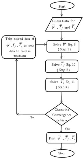
Figure 1.
Flowchart of conventional solution methodology.
The whole process requires the solution be completed in three steps corresponding to three equations. However, the current paper deals in the solution of the three equations in two steps by combining the energy equation of the fluid and solid into a single stiffness matrix, which results in a 3 × 3 stiffness matrix for the momentum equation and a 6 × 6 matrix for the energy equation. Combined stiffness matrix of the energy equation for the fluid and solid can be written as:
where
This arrangement leads to the reduction of three equations into a two-equation problem whose solution can be obtained by following the procedure shown in Figure 2. The computer coding of the new method is easier due to the removal of one complete subroutine required to solve the energy equation.
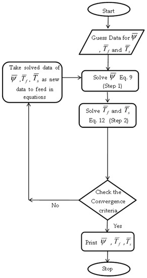
Figure 2.
Flowchart of new method.
3. Results and Discussion
Any new method should be able to withstand the test of simulating the physical problem. Thus, the proposed new method is tested by applying to heat transfer in a square porous cavity. The physical domain of the porous medium to be tested is shown in Figure 3, which has been subjected to assumptions that the fluid follows Darcy’s law, that the porous medium is saturated with fluid, that the fluid and medium are not in local thermal equilibrium, that the porous medium is isotropic and homogeneous, and that the fluid properties are constant except for the variation of density. The physical domain is divided into 2592 elements of a triangular shape. Mesh independency is ensured before selecting 2592 elements to make sure that the results are not affected even if more elements are chosen. Smaller-sized elements are placed at the boundaries where large variations are expected as compared to regions away from the boundaries. The applied boundary conditions are given below.
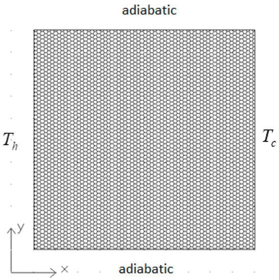
Figure 3.
Porous domain.
There can be many solution methods, but their usability should be established by verifying them to accurately predict the given phenomenon. Thus, the proposed method is tested against the data available in open literature. The results obtained for the case of square porous cavity subjected to non-equilibrium condition is compared and shown in Figure 4 and Figure 5 and Table 1. Figure 4 corresponds to Ra = 100, Rd = 0.5, and Kr = 1. The parameter Kr represents the thermal conductivity ratio between fluid and solid phases of the porous medium. It is clear from Figure 4 and Figure 5 that the isotherms of the solid phase and fluid phase along with streamline match very well with published data. The method is further validated with the Nusselt number of fluids, solids, and the total Nusselt number, as shown in Table 1. It is clear from this table that the present method can predict the heat transfer from the hot surface to the porous medium accurately. The proposed method is further analyzed to predict the limiting case of thermal equilibrium. It is well known that the existence of the high thermal conductivity ratio “Kr” and higher value of interphase heat transfer coefficient “H” leads to thermal equilibrium between solid and fluid phases due to better heat exchange between the two phases. The proposed method should be tested against this limiting case. Figure 6 and Table 2 illustrates the validation of the thermal equilibrium condition. Figure 6 shows the isotherms of the fluid and solid phase when Kr = 1000 and H = 1000. It is very clear from this figure that the isotherms of both phases are very similar to each other, which indicates that the thermal equilibrium condition prevails at higher values of Kr and H. Therefore, this validates the capability of the proposed method. The average Nusselt number for the equilibrium condition is also compared (Table 2) with data available in the literature. It was convincingly found that the proposed method has good accuracy in predicting the Nusselt number.
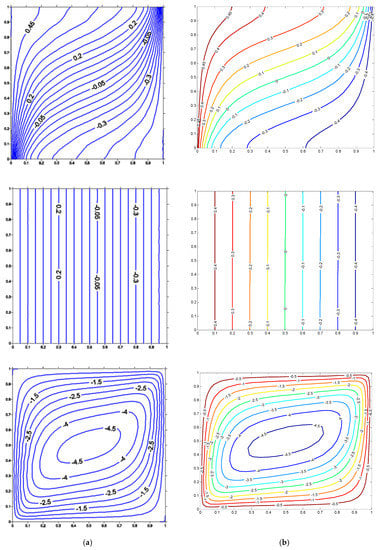
Figure 4.
Isotherms for fluid (Top), solid (Middle), and streamlines (Bottom) at Ra = 100, Rd = 0.5, Kr = 1, H = 0.1, (a) Ref [27]. (b) Present.
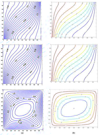
Figure 5.
Isotherms for fluid (Top), solid (Middle), and streamlines (Bottom) at Ra = 100, Rd = 0.5, Kr = 1, H = 1000, (a) Ref [27] (b) Present.

Table 1.
Comparison of Nusselt number at Ra = 100, Kr = 50, and Rd = 0.5.
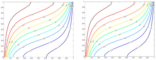
Figure 6.
Isotherms for fluid (Left) and solid (Right) at the equilibrium condition, Ra = 100, Rd = 0.5, Kr = 1000, H = 1000.
Table 2.
Validation of the average Nusselt number, for the equilibrium condition.
3.1. Thermal Non-Equilibrium Analysis of Porous Cavity Due to the Heated Strip
The developed solution method is used to investigate the thermal non-equilibrium in a porous cavity having a vertical heated strip inside the porous domain. The investigation is carried out for two cases such that case I belongs to heat being supplied to porous medium through an isothermally heated strip along with the left as well as the right vertical surfaces of the cavity being maintained at a cold temperature. Case II is considered in such a way that the left vertical surface of the cavity is also heated to a hot temperature apart from the heated strip. The right vertical surface is maintained at a cold isothermal temperature. The top and bottom surfaces are adiabatic in both cases.
3.2. Case I
The boundary conditions in dimensional form for case I can be expressed as:
The usage of non-dimensional parameters results in:
The Nusselt number is calculated according to the formulas below.
Figure 7, Figure 8, Figure 9, Figure 10, Figure 11 and Figure 12 show the isotherms of fluid, solid, and stream line characteristics derived for various geometrical and physical parameters. The first and second row of each of these figures shows the fluid and solid phase isotherms, respectively, with the last row reflecting the streamline variations. It is expectedly observed for all these figures that the heat transfer and fluid flow follow symmetrical behavior for the heating strip when placed at the center but unsymmetrical behavior when the strip departs from the central position. Figure 7 depicts the heat transfer and fluid flow characteristics when the length of the strip varies from 12.5% to 50% of the cavity height. The fluid isotherms indicate the convection of heat due to movement of the fluid arising because of density variation. The increase in the strip height leads to larger variation in the fluid isotherms. It must be noted that the increase in the strip height would bring in more thermal energy because of the larger area of porous medium being exposed to the heated strip. This leads to higher variation in the fluid temperature across the porous domain. The solid phase isotherms get affected when the strip height HH is increased. The smaller strip leads to a larger area of the porous domain that needs to be occupied with low temperature lines with a small thermal gradient across the domain. However, the increased strip height leads to a higher thermal gradient and better conduction across the domain. The streamlines clearly indicate that the fluid velocity grows with an increase in strip height, which is reflected in terms of a higher magnitude of stream function at HH = 0.5 as compared to HH = 0.125.
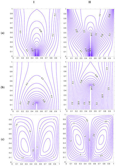
Figure 7.
Isotherms ((a) Fluid, (b) Solid) and streamlines (c), at Ra = 100, H = 5, Kr = 1, Rd = 0 for strip at . (I) HH = 12.5%. (II) HH = 50%.
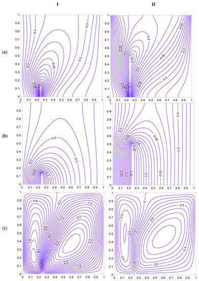
Figure 8.
Isotherms ((a) Fluid, (b) Solid) and streamlines (c), at Ra = 100, H = 5, Kr = 1, Rd = 0 for strip at . (I) HH = 12.5%. (II) HH = 50%.
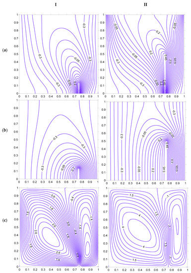
Figure 9.
Isotherms ((a) Fluid, (b) Solid), and streamlines (c), at Ra = 100, H = 5, Kr = 1, Rd = 0 for strip at . (I) HH = 12.5%. (II) HH = 50%.
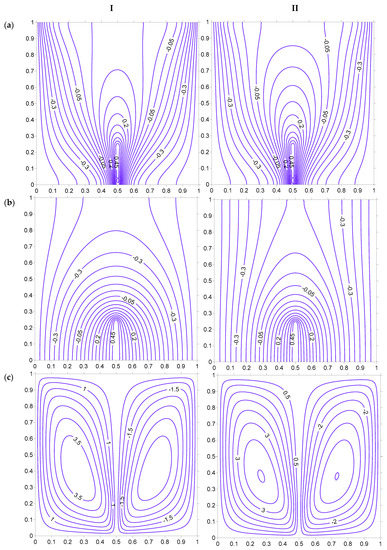
Figure 10.
Isotherms ((a) Fluid, (b) Solid), and streamlines (c), at Ra = 100, HH = 25%, Kr = 1, Rd = 0 for strip at . (I) H = 0.1. (II) H = 10.
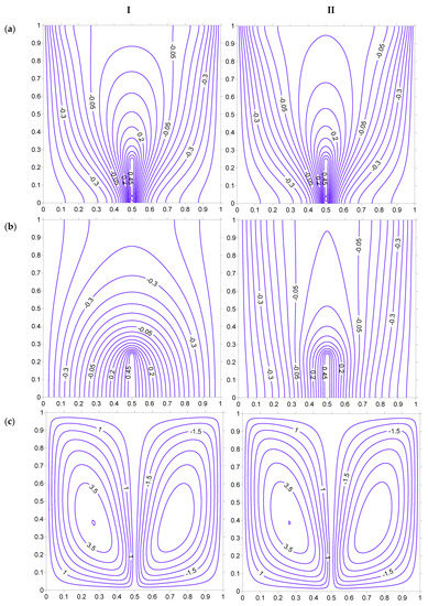
Figure 11.
Isotherms ((a) Fluid, (b) Solid), and streamlines (c), at Ra = 100, HH = 25%, H = 5, Rd = 0 for strip at . (I) Kr = 0.1. (II) Kr = 10.
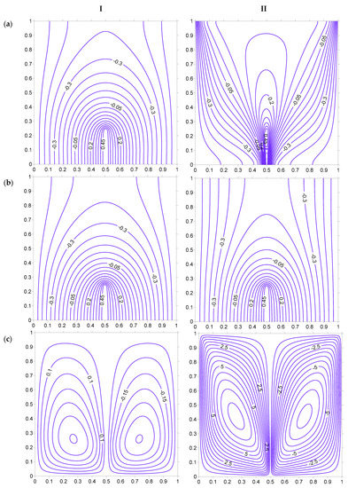
Figure 12.
Isotherms ((a) Fluid, (b) Solid), and streamlines (c), at H = 5, HH = 25%, Kr = 1, Rd = 0 for strip at . (I) Ra = 100. (II) Ra = 200.
The change of position of the strip brings in pronounced variation in heat transfer behavior as shown in Figure 8, when compared to that of Figure 7. In this figure, the heating strip is placed toward the left vertical surface at . The fluid isotherms create a higher thermal gradient toward the left vertical surface than the right vertical surface. This clearly indicates that the heat dissipation is higher toward the left surface of the cavity than the right surface. A substantial area toward the right of the heating strip is seen to have low temperature lines due to lower thermal energy in that vicinity. This situation improves slightly with the increase in the strip height to 50%. The fluid flows in a vertical direction at the left surface, but in an oblique cell toward the right region of the heated strip. The change in the strip’s position () toward the right vertical surface, as shown in Figure 9, has similar behavior to the results in Figure 8 but with the higher thermal gradient being created toward the right surface and the lower gradient being created toward the left surface.
The following three figures, i.e., Figure 10, Figure 11 and Figure 12, illustrate the effect of variation of physical parameters such as the interphase heat transfer coefficient H, the thermal conductivity ratio Kr, and the Rayleigh number Ra. Figure 10 shows the H being changed from 0.1 to 10. The increase in the interphase heat transfer coefficient is known to have similarity between the fluid and solid phase [8,21], which leads toward a thermal equilibrium condition. In the present case as well, it is noted that the dissimilarity reduces between the fluid and solid phase when H is increased from 0.1 to 10, even though a thermal equilibrium condition is not yet reached. The thermal equilibrium is expected to reach a much higher value of H. The temperature gradient of fluid decreases while, that of the solid phase, increases near the hot strip when H is increased. This can be observed through the fluid and solid isotherms where the fluid temperature lines move away from the strip and the solid temperature lines come closer to the strip. The increased value of H leads to better transfer of heat between the two phases. Thus, the fluid loses the heat to the solid matrix, which reduces fluid temperature and increases that of the solid matrix.
Figure 11 shows the impact of increasing the thermal conductivity ratio between the fluid and solid phase. In this case, the dissimilarity between fluid and solid phases decreases due to the increased value of Kr. It must also be noted that the large value of Kr leads to a thermal equilibrium condition. The higher value of Kr helps the heat to be conducted in a better way in the solid matrix of porous medium, which leads to straighter isotherms (reflecting better conduction) of the solid phase. Figure 12 shows the effect of the Rayleigh number on heat transfer behavior of a square porous domain. The fluid isotherms are distorted due to an increase in the Rayleigh number from 100 to 200, which indicates that the convection heat transfer increases in the fluid phase. The streamlines are crowded with higher magnitude that indicates the increased fluid velocity due to a higher Rayleigh number.
Figure 13, Figure 14, Figure 15, Figure 16, Figure 17 and Figure 18 shows the Nusselt number variation for the previously mentioned parameters. Figure 13 illustrates the local Nusselt number of the fluid and solid phase. It must be noted that there would be two Nusselt number values of fluid as well as solid phases corresponding to the left and right side of the heating strip. However, the symmetric placement of the heating strip ensures that the Nusselt number values are identical toward the left and right side of the heater. For instance, when the heating strip is placed at , then the left and right side of the Nusselt number is identical due to symmetrical geometry and boundary conditions. When the strip is placed at , then the Nusselt number at the right side of the strip is similar to Nu corresponding to the left side of the strip at . Thus, only one value of the Nusselt number, i.e., left of the heating strip, is presented in Figure 13, Figure 14, Figure 15, Figure 16, Figure 17 and Figure 18.
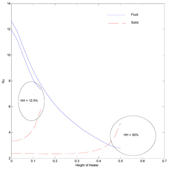
Figure 13.
Nusselt number at Ra = 100, H = 5, Kr = 1, Rd = 0 for strip at .
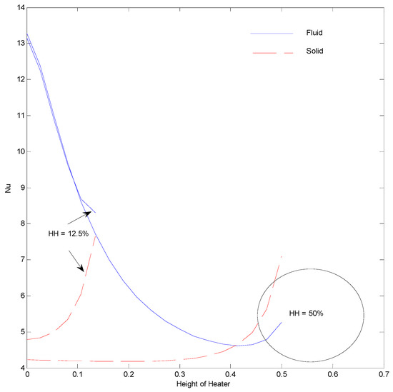
Figure 14.
Nusselt number at Ra = 100, H = 5, Kr = 1, Rd = 0 for strip at .
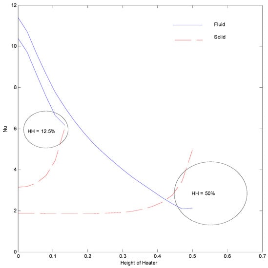
Figure 15.
Nusselt number at Ra = 100, H = 5, Kr = 1, Rd = 0 for strip at .
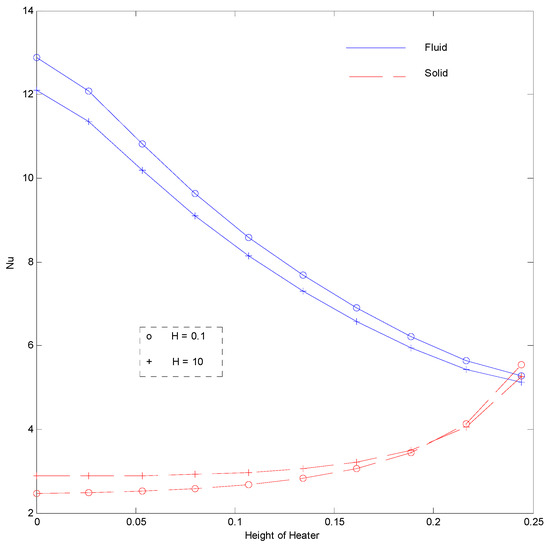
Figure 16.
Nusselt number at Ra = 100, HH = 25%, Kr = 1, Rd = 0 for strip at .
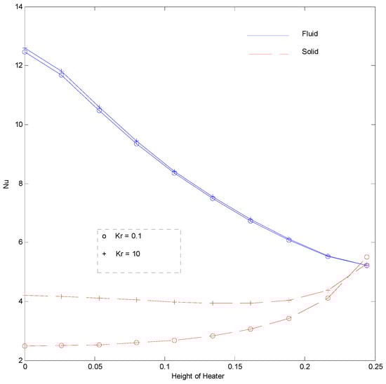
Figure 17.
Nusselt number at Ra = 100, HH = 25%, H = 5, Rd = 0 for strip at .
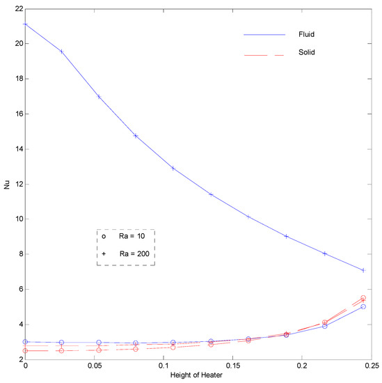
Figure 18.
Nusselt number at H = 5, HH = 25%, Kr = 1, Rd = 0 for strip at .
The Nusselt number of fluid (Figure 13) is found to decrease along the height of the heating strip, which is the result of the increase in the temperature of fluid as it moves along the heated strip. This increased fluid temperature reduces the temperature difference between the strip and fluid near its vicinity, which reduces the thermal gradient. The solid Nusselt number increases along the height of the Strip. This is the direct result of a higher temperature gradient created in the solid phase along the strip height, as vindicated by isotherms of Figure 7. It can be seen in Figure 7 that the solid isotherms tend to come closer to the strip at the upper section of the strip as compared to its lower section. The increase in strip height from 12.5% to 50% leads to an almost constant Nusselt number of solid until the top of the strip and then t increases. This is reflected by almost parallel solid phase isotherms along most of the solid strip in Figure 7. It is also noted that the solid Nusselt number overtakes the fluid Nusselt number at the upper section of the strip. The placement of the heating strip near the left surface increases the Nusselt number for fluid as well as the solid phase, in comparison to that of the heating strip at the central position. This can be attributed to the fact that the thermal resistance decreases due to less distance between the heating strip and the cold surface. This should help the electronic devices where the power source can be placed toward the cold surface for better dissipation of heat. The placement of the strip toward the right surface reduces the heat transfer, which is reflected in terms of a reduced Nusselt number of fluid and solid phases, as shown in Figure 14. This happens due to a larger distance between the strip and the cold surface that leads to increased thermal resistance. Thus, it can be said that the Nusselt number is highest when the distance between the strip and surface is the lowest (Figure 14) and the lowest when the distance is the highest (Figure 15).
Figure 16 shows that the fluid Nusselt number decreases and the solid Nusselt number increases with a rise in the interphase heat transfer coefficient. It can be inferred through the isotherms of fluid and solid that the fluid gains heat from the solid phase of porous medium due to a better heat transfer coefficient (larger H). The heat gain from solid to fluid increases the fluid temperature but reduces that of the solid, which reduces the thermal gradient of fluid and increases the thermal gradient of solid. Figure 17 illustrates the effect of the thermal conductivity ratio of the Nusselt number. The fluid Nusselt number is not affected much, but the solid phase Nusselt number increases with an increase in Kr. This behavior is consistent with the other studies reported [23]. The Nusselt number of fluid is substantially increased when the Rayleigh number is increased (Figure 18), but that of solid is increased to a slight extent. This is because the fluid movement increases with a rise in the Rayleigh number that, in turn, increases the heat carrying capacity of fluid, which increases the fluid Nusselt number.
3.3. Case II
This section describes the heat transfer behavior when the left vertical surface is also heated to a hot temperature along with the heating strip placed inside the porous domain. The boundary conditions for this case can be expressed by the following.
The usage of non-dimensional parameters results in:
Figure 19, Figure 20, Figure 21, Figure 22, Figure 23 and Figure 24 illustrate the isotherms and streamlines due to heating of the left vertical surface along with the heated strip, which is placed in the porous domain. The heat transfer behavior is affected substantially in this case as compared to that of the previously mentioned case (Case I). The heating of the left surface of the cavity results in unsymmetrical distribution of isotherms and streamlines, which is different from that of Case I. The increase in the strip height ensures that the temperature variations at the left half of the cavity are minimal (Figure 19). The left half of the cavity has higher energy content, as indicated by fluid and solid isotherms. The increase in the strip height leads to a substantial portion of the cavity at the left side of the heated strip without any fluid movement, as indicated by the streamline in Figure 19. The placement of the heated strip to the left side () as shown in Figure 20, restricts the high temperature area to about 25% of the porous cavity. However, the temperature variations at the right side of the strip decreases in this case, as compared to the strip being placed at (Figure 19). The further shift of the strip to brings the isotherms closer to each other at the right side of the strip, as shown in Figure 21. The fluid flows rapidly within the small region between the strip and the right cold surface, but slowly left of the heated strip. The smaller-sized strip allows the fluid to be occupied in almost all of the cavity but an increase in strip height reduces the fluid flow area, as shown by the streamlines of Figure 19, Figure 20 and Figure 21.
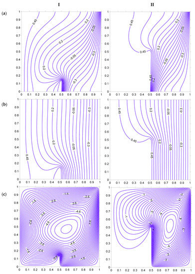
Figure 19.
Isotherms ((a) Fluid, (b) Solid), and streamlines (c), at Ra = 100, H = 5, Kr = 1, Rd = 0 for strip at . (I) HH = 12.5%. (II) HH = 50%.
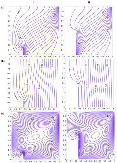
Figure 20.
Isotherms ((a) Fluid, (b) Solid), and streamlines (c), at Ra = 100, H = 5, Kr = 1, Rd = 0 for strip at . (I) HH = 12.5%. (II) HH = 50%.
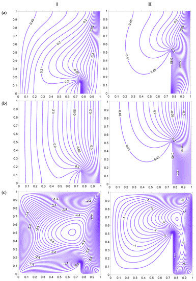
Figure 21.
Isotherms ((a) Fluid, (b) Solid), and streamlines (c), at Ra = 100, H = 5, Kr = 1, Rd = 0 for strip at . (I) HH = 12.5%. (II) HH = 50%.
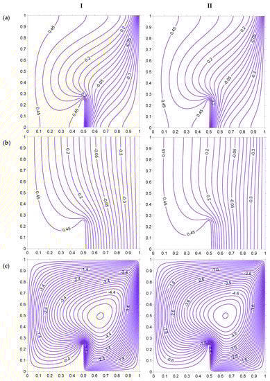
Figure 22.
Isotherms ((a) Fluid, (b) Solid), and streamlines (c), at Ra = 100, HH = 25%, Kr = 1, Rd = 0 for strip at . (I) H = 0.1. (II) HH = 10.
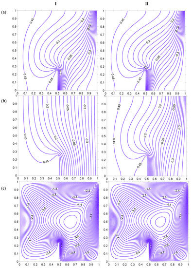
Figure 23.
Isotherms ((a) Fluid, (b) Solid), and streamlines (c), at Ra = 100, HH = 25%, Kr = 1, Rd = 0 for strip at . (I) Kr = 0.1. (II) Kr = 10.
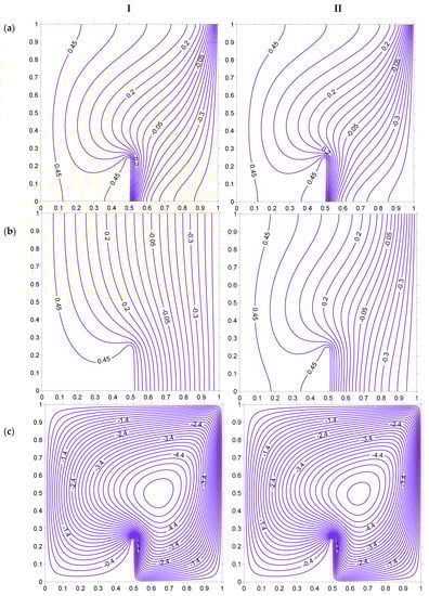
Figure 24.
Isotherms ((a) Fluid, (b) Solid), and streamlines (c), at HH = 25%, H = 5, Kr = 1, Rd = 0 for strip at . (I) Ra = 100. (II) Ra = 200.
Figure 22 shows the effect of the interphase heat transfer coefficient H on isotherms and streamline for Case II. The increase in the H pushes the isotherms toward the right surface, which can be inferred by looking at the isotherm corresponding to 0.45. The streamline magnitude increases with a rise in H. The magnitude of streamline is higher in this case as compared to Case I. The influence of the thermal conductivity ratio is illustrated in Figure 23. The fluid temperature is not affected much by the change in the thermal conductivity ratio, but solid temperature lines are affected to a certain extent. The increase in Kr leads to larger temperature variations of the solid phase in the porous domain. The increase in the Rayleigh number leads to a large number of fluid isotherms being crowded near the right side of the heated strip (Figure 24). This should lead to a substantial increase in heat transfer toward the right side of the heated strip. This behavior is not observed at the left side of the heated strip. It can be inferred that the heated left vertical surface of the cavity does not allow the isotherms to be crowded near the strip, which happens in case I.
Figure 25, Figure 26, Figure 27, Figure 28, Figure 29 and Figure 30 shows the local Nusselt number for fluid and solid corresponding to Case II. It must be noted that the heat transfer from the heated strip to the porous medium differs toward the left and right side of the strip. Thus, two values of the Nusselt number is plotted to illustrate this effect. Figure 25 shows the Nusselt number for strip height to be 12.5 and 50% of the cavity height. The Nusselt number is lower at the left side of the strip than the right side for fluid as well as the solid phase. This happens because the cold surface is located at the right of the strip, which allows the heat to be dissipated to a cold surface that, in turn, creates an opportunity for further heat transfer. However, this does not happen between the strip and the hot surface of the cavity. Due to heat flowing from the strip as well as the left surface, the temperature in that area increases, which reduces the heat transfer rate as reflected in the reduced Nusselt number. Figure 26 shows the heat transfer behavior from the left vertical surface of the cavity. The heat transfer from the left surface is higher when the strip is shorter in height. The longer strip height blocks the heat flow from the left vertical surface toward the cold surface (right vertical surface). Thus, the Nusselt number is higher when the strip is shorter. It is also observed that the solid phase Nusselt number is higher all along the surface for a longer strip. This can be attributed to the fact that the fluid flow gets blocked when the strip is longer, which, in turn, weakens the heat carrying capacity from the left hot surface to the right cold surface. However, for the shorter strip, fluid has a sufficient open space to travel from a hot to a cold vertical surface. This increases the fluid heat transfer rate.
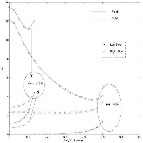
Figure 25.
Nusselt number for inner strip at Ra = 100, H = 5, Kr = 1, Rd = 0 for strip at .
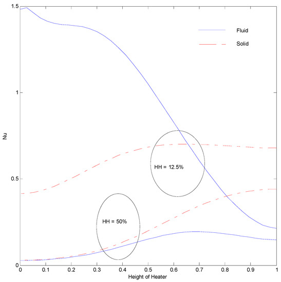
Figure 26.
Nusselt number of left vertical surface at Ra = 100, H = 5, Kr = 1, Rd = 0 for strip at .
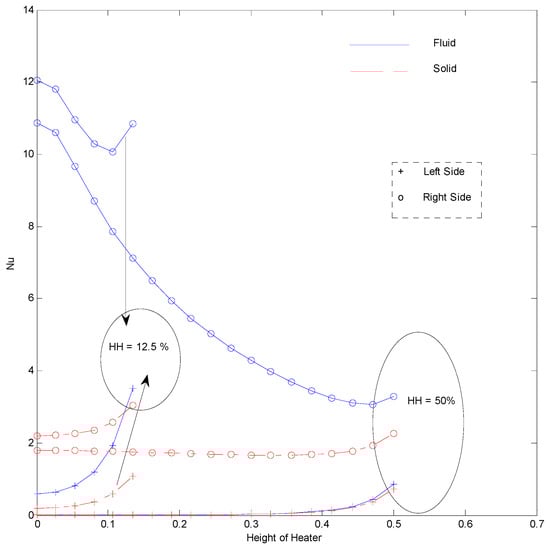
Figure 27.
Nusselt number for inner strip at Ra = 100, H = 5, Kr = 1, Rd = 0 for strip at .
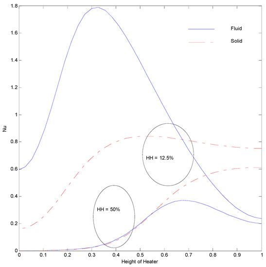
Figure 28.
Nusselt number of the left vertical surface at Ra = 100, H = 5, Kr = 1, Rd = 0 for strip at .
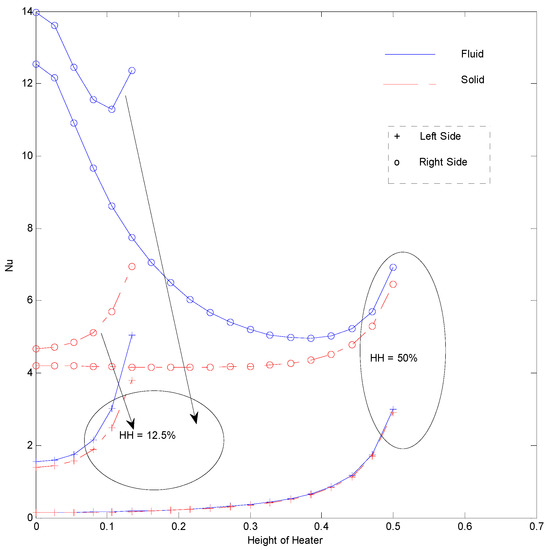
Figure 29.
Nusselt number for inner strip at Ra = 100, H = 5, Kr = 1, Rd = 0 for strip at .
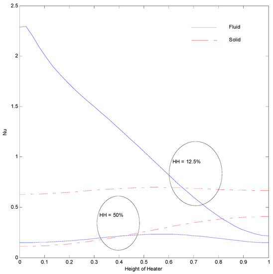
Figure 30.
Nusselt number of left vertical surface at Ra = 100, H = 5, Kr = 1, Rd = 0 for strip at .
Figure 27 illustrates the impact of moving the strip to the left of the cavity (). The Nusselt number on the right side of the strip follows a similar trend as that of Figure 25. However, the maximum value of the Nusselt number in this case is lower than that of the strip being placed at the central position (Figure 25). This is due to the increased distance between the strip and the cold surface, which reduces the heat transfer rate. The heat transfer at the left vertical surface for the fluid phase was found to increase until a certain height of the cavity and then decreased, as shown in Figure 28. This behavior is unique for the cases when the strip is placed closer to the vertical hot surface. This can be related to the fluid cell circulation inclined toward the left bottom and the right top corner of the cavity, which creates a faster circulation zone near the , as illustrated in Figure 20. However, this kind of variation is not seen for the solid phase Nusselt number. Figure 29 and Figure 30 shows the Nusselt number variation at the inner heater and the left vertical surface, respectively, when the strip is placed at the right side of the cavity at . The heat transfer from the strip to the porous medium is higher in this case because of proximity of lower temperature surface (cold surface), which facilitates better heat transfer. Figure 30 illustrates that the heat transfer from the left hot surface decreases almost linearly along the surface for 12.5% of the strip height, when the strip is placed near the cold surface. However, the longer strip almost ceases the Nusselt number variation of fluid due to decreased fluid movement, which can be inferred from the reduced magnitude of streamlines between the left vertical surface and the strip (Figure 21).
4. Conclusions
The present article proposes an alternate method to solve the two-heat transport equations of the thermal non-equilibrium model in a simpler algorithm by utilizing the finite element method as a base tool. The fluid and solid phase equations are combined in a single stiffness matrix at the solution stage. The proposed method is tested for heat transfer in a porous cavity. It is found that the proposed method is very capable of predicting the thermal equilibrium as well as non-equilibrium condition. The proposed method is used to investigate the heat transfer due to a heating strip being placed inside the porous domain. Two different boundary conditions are studied. The heat transfer is highest when the position of the heating strip is closer to the cold surface. The longer strip is found to decrease heat transfer when the left vertical surface is also heated to a higher temperature. The heat transfer from the strip is found to be higher toward the cold surface and lower toward the hot vertical surface. The Nusselt number for Case I with heating strip at and strip height 12.5%, is found to be 13.28. However, this value drops to 0.59 when the left vertical surface is also heated (Case II). This difference of the Nusselt number was even higher for a strip height of 50%. This study revealed that there can be substantial variations in heat transfer due to strip height and the location. It would be interesting to extend this study for mixed/forced convection that occurs in some of the electronic devices.
Funding
The King Khalid University, under the grant number R.G.P. 1/85/40, funded this research.
Acknowledgments
The author extends his appreciation to the Deanship of Scientific Research at King Khalid University for funding this work through the research group program under grant number (R.G.P. 1/85/40).
Conflicts of Interest
There is no conflict of interest.
Nomenclature
| A | Element area |
| g | Acceleration due to gravity (m/s2) |
| h | Heat transfer coefficient (W/m2·C) |
| k | Thermal conductivity (W/m·°C) |
| kp, ks | Porous and solid thermal conductivity respectively (W/m·°C) |
| HH | Strip height |
| K | Permeability of porous medium (m2) |
| Kr = ks/kp | Conductivity ratio |
| L | Height and length of cavity (m) |
| Radiation parameter | |
| Modified Raleigh number | |
| Temperature | |
| u,v | Velocity component sin x and y direction respectively (m/s) |
| Cartesian coordinates | |
| Non-dimensional coordinates | |
| Greek Symbols | |
| α | Thermal diffusivity (m2/s) |
| β | Coefficient of thermal expansion (1/°C) |
| ρ | Density (kg/m3) |
| v | Coefficient of kinematic viscosity (m2/s) |
| Stephan Boltzmann constant (W/m2·K4) | |
| Absorption coefficient (1/m) | |
| Stream function | |
| Non-dimensional stream function | |
| Subscripts | |
| h | Hot |
| c | Cold |
| s | Solid |
| f | Fluid |
References
- Segerland, L.J. Applied Finite Element Analysis; John Wiley and Sons: New York, NY, USA, 1982. [Google Scholar]
- Lewis, R.W.; Morgan, K.; Thomas, H.R.; Seetharamu, K.N. The Finite Element Method in Heat Transfer Analysis; John Wiley & Sons: Chichester, UK, 1996. [Google Scholar]
- Ahmed, N.S.; Badruddin, I.A.; Kanesan, J.; Zainal, Z.A.; Ahamed, K.N. Study of mixed convection in an annular vertical cylinder filled with saturated porous medium, using thermal non-equilibrium model. Int. J. Heat Mass Transf. 2011, 54, 3822–3825. [Google Scholar] [CrossRef]
- Badruddin, I.A.; Al-Rashed, A.A.; Ahmed, N.S.; Kamangar, S.; Jeevan, K. Natural convection in a square porous annulus. Int. J. Heat Mass Transf. 2012, 55, 7175–7187. [Google Scholar] [CrossRef]
- Amiri, A.; Vafai, K. Transient analysis of incompressible flow through a packed bed. Int. J. Heat Mass Transf. 1998, 41, 4259–4279. [Google Scholar] [CrossRef]
- Jiang, P.X.; Ren, Z.P. Numerical investigation of forced convection heat transfer in porous media using a thermal non-equilibrium model. Int. J. Fluid Flow 2001, 22, 102–110. [Google Scholar] [CrossRef]
- Wong, S.W.; Rees, D.A.S.; Pop, I. Forced convection past a heated cylinder in a porous medium using a thermal non-equilibrium model: Finite Peclet number effects. Int. J. Therm. Sci. 2004, 43, 213–220. [Google Scholar] [CrossRef]
- Rajamani, R.; Srinivasa, C.; Nitiarasu, P.; Seetharamu, K.N. Convective heat transfer in axisymmetric porous bodies. Int. J. Numer. Methods Heat Fluid Flow 1995, 5, 829–837. [Google Scholar] [CrossRef]
- Balla, C.S.; Naikoti, K. Soret and Dufour effects on free convective heat and solute transfer in fluid saturated inclined porous cavity. Eng. Sci. Technol. Int. J. 2015, 18, 543–554. [Google Scholar] [CrossRef]
- Badruddin, I.A.; Zainal, Z.A.; Aswatha Narayana, P.A.; Seetharamu, K.N. Thermal non-equilibrium modeling of heat transfer through vertical annulus embedded with porous medium. Int. J. Heat Mass Transf. 2006, 49, 4955–4965. [Google Scholar] [CrossRef]
- Mahmoudi, Y. Effect of thermal radiation on temperature differential in a porous medium under local thermal non-equilibrium condition. Int. J. Heat Mass Transf. 2014, 76, 105–121. [Google Scholar] [CrossRef]
- Bera, P.; Pippal, S.; Sharma, A.K. A thermal non-equilibrium approach on double-diffusive natural convection in a square porous-medium cavity. Int. J. Heat Mass Transf. 2014, 78, 1080–1094. [Google Scholar] [CrossRef]
- Baytas, A.C.; Pop, I. Free convection in a square porous cavity using a thermal nonequalibruim model. Int. J. Therm. Sci. 2002, 41, 861–870. [Google Scholar] [CrossRef]
- Sheremet, M.; Pop, I.; Baytas, A. Non-equilibrium natural convection in a differentially-heated nanofluid cavity partially filled with a porous medium. Int. J. Numer. Methods Heat Fluid Flow 2019, 29, 2524–2544. [Google Scholar] [CrossRef]
- Abdollahzadeh, J.M.; Oveisi, M. Local thermal non-equilibrium forced convection of a third grade fluid between parallel stretching permeable plates embedded in a porous medium. Therm. Sci. 2019, 23, 475–484. [Google Scholar] [CrossRef]
- Rajarathinam, M.; Nithyadevi, N. Magneto convection heat transfer in a porous square cavity using local thermal non-equilibrium approach. Spec. Top. Rev. Porous Media Int. J. 2019, 10, 129–141. [Google Scholar] [CrossRef]
- Alizadeh, R.; Karimi, N.; Nourbakhsh, A. Effects of radiation and magnetic field on mixed convection stagnation-point flow over a cylinder in a porous medium under local thermal non-equilibrium. J. Therm. Anal. Calorim. 2019. [Google Scholar] [CrossRef]
- Saeid, N.H. Analysis of free convection about a horizontal cylinder in a porous media using a thermal non-equilibrium model. Int. Commun. Heat Mass Transf. 2006, 33, 158–165. [Google Scholar] [CrossRef]
- Saeid, N.H. Analysis of mixed convection in a vertical porous layer using non-equilibrium model. Int. J. Heat Mass Transf. 2004, 47, 5619–5627. [Google Scholar] [CrossRef]
- Espinosa-Paredes, G.; Vázquez-Rodríguez, A.; Espinosa-Martínez, E.G.; Cazarez-Candia, O.; Viera, M.D.; Moctezuma-Berthier, A. A numerical analysis of non-equilibrium thermodynamic effects in an oil field: Two-equation model. Pet. Sci. Technol. 2013, 31, 192–203. [Google Scholar] [CrossRef]
- Vadasz, P. Explicit conditions for local thermal equilibrium in porous media heat conduction. Transp. Porous Media 2005, 59, 341–355. [Google Scholar] [CrossRef]
- Omara, A.; Bourouis, A.; Abboudi, S. Numerical Approach of Thermal non Equilibrium Natural Convection in a Square Porous Cavity with Partially Thermally Active Side Walls. J. Appl. Fluid Mech. 2016, 9, 223–233. [Google Scholar]
- Rees, D.A.S. Microscopic modelling of the two-temperature model for conduction in heterogeneous media. J. Porous Media 2010, 13, 125–143. [Google Scholar] [CrossRef]
- Rees, D.A.S. The effect of local thermal non-equilibrium on the stability of convection in a vertical porous channel. Transp. Porous Media 2011, 87, 459–464. [Google Scholar] [CrossRef]
- Nicolas, L.S.; Straughan, B. A Nonlinear Stability Analysis of Convection in a Porous Vertical Channel Including Local Thermal Nonequilibrium. J. Math. Fluid Mech. 2013, 15, 171–178. [Google Scholar]
- Straughan, B. Global nonlinear stability in porous convection with a thermal nonequilibrium model. Proc. R. Soc. A 2006, 462, 409–418. [Google Scholar] [CrossRef]
- Badruddin, I.A.; Zainal, Z.A.; Aswatha Narayana, P.A.; Seetharamu, K.N. Numerical analysis of convection conduction and radiation using a non-equilibrium model in a square porous cavity. Int. J. Therm. Sci. 2007, 46, 20–29. [Google Scholar] [CrossRef]
- Manole, D.M.; Lage, J.L. Numerical benchmark results for natural convection in a porous medium cavity. In Proceedings of the Heat and Mass Transfer in Porous Media, ASME Conference, HTD 216, Anaheim, CA, USA, 8–13 November 1992; pp. 55–60. [Google Scholar]
- Bekermann, C.; Viskanta, R.; Ramadhyani, S. A numerical study of non-Darcian natural convection in a vertical enclosure filled with a porous medium. Numer. Heat Transf. Part A 1986, 10, 557–570. [Google Scholar]
- Walker, K.L.; Homsy, G.M. Convection in a porous cavity. J. Fluid Mech. 1978, 87, 449–474. [Google Scholar] [CrossRef]
- Bejan, A. On the boundary layer regime in a vertical enclosure filled with a porous medium. Lett. Heat Mass Transf. 1979, 6, 93–102. [Google Scholar] [CrossRef]
- Gross, R.J.; Bear, M.R.; Hickox, C.E. The application of flux-corrected transport (FCT) to high Rayleigh number natural convection in a porous medium. In Proceedings of the 8th International Heat Transfer Conference, San Francisco, CA, USA, 17–22 August 1986. [Google Scholar]
- Moya, S.L.; Ramos, E.; Sen, M. Numerical study of natural convection in a tilted rectangular porous material. Int. J. Heat Mass Transf. 1987, 30, 741–756. [Google Scholar] [CrossRef]
- Baytas, A.C.; Pop, I. Free convection in oblique enclosures filled with a porous medium. Int. J. Heat Mass Transf. 1999, 42, 1047–1057. [Google Scholar] [CrossRef]
- Misirlioglu, A.; Baytas, A.C.; Pop, I. Free convection in a wavy cavity filled with a porous medium. Int. J. Heat Mass Transf. 2005, 48, 1840–1850. [Google Scholar] [CrossRef]
© 2019 by the author. Licensee MDPI, Basel, Switzerland. This article is an open access article distributed under the terms and conditions of the Creative Commons Attribution (CC BY) license (http://creativecommons.org/licenses/by/4.0/).