Cournot Duopoly Games: Models and Investigations


Abstract
1. Introduction
2. Model 1
3. Local Analysis
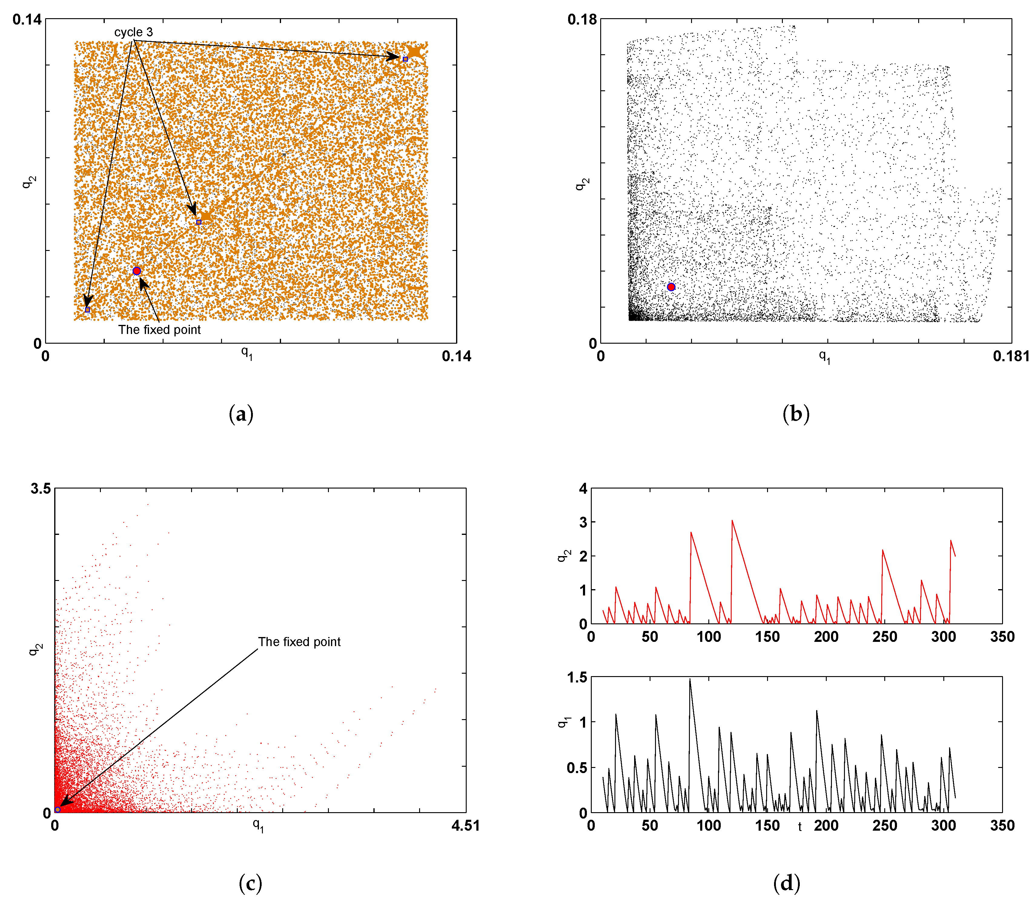
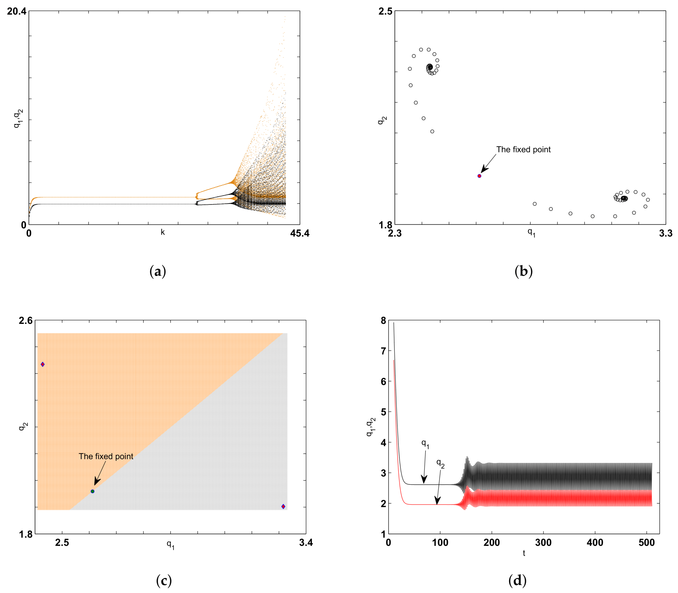
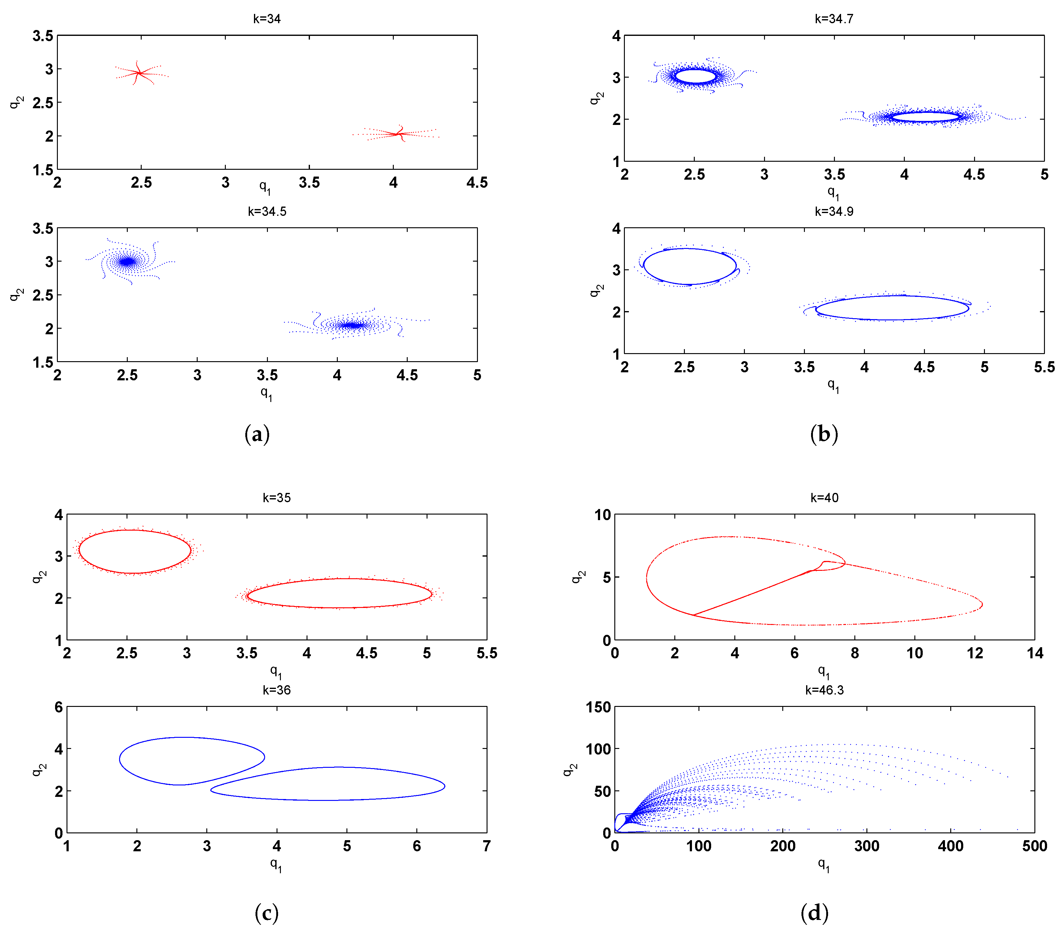
Numerical Simulation and Global Analysis
4. Model 2
4.1. Dynamic Adjustment
Numerical Simulation
4.2. Tit-for-Tat Mechanism
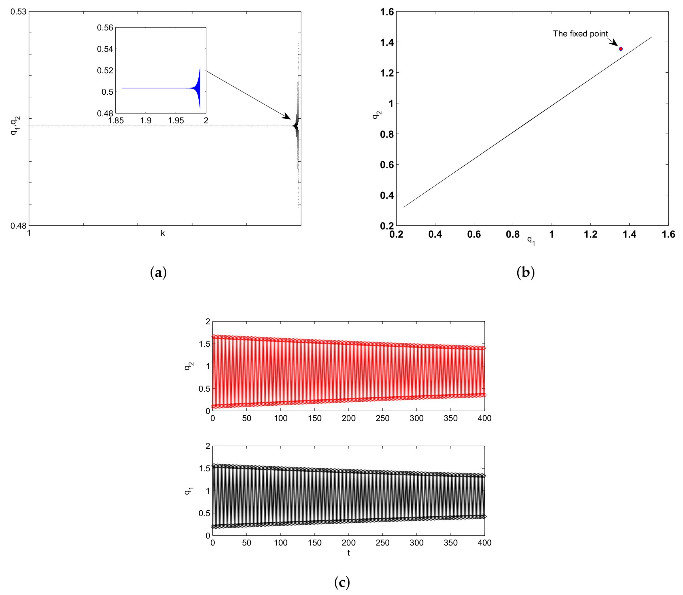
Numerical Simulation
5. Conclusions
Author Contributions
Funding
Acknowledgments
Conflicts of Interest
References
- Cournot, A.A. Researches into the principles of the theory of wealth. In Classics in Economics; Augustus M Kelley Pubs.: New York, NY, USA, 1971. [Google Scholar]
- Cavalli, F.; Namizada, A.; Tramontana, F. Nonlinear dynamics and global analysis of a heterogeneous Cournot duopoly with a local monopolistic approach versus a gradient rule with endogenous reactivity. Commun. Nonlinear Sci. Numer. Simul. 2015, 23, 245–262. [Google Scholar] [CrossRef]
- Rand, D. Exotic phenomena in games and duopoly models. Math. Econ. 1978, 5, 173–184. [Google Scholar] [CrossRef]
- Poston, T.; Stewart, I. Catastrophe Theory and Its Applications; Pitman Ltd.: London, UK, 1978. [Google Scholar]
- Naimzada, A.; Sbragia, L. Oligopoly games with nonlinear demand and cost functions: Two boundedly rational adjustment processes. Chaos Solitons Fractals 2006, 29, 707–722. [Google Scholar] [CrossRef]
- Askar, S.S. Dynamic Cournot duopoly games with nonlinear demand function. Appl. Math. Comput. 2015, 259, 427–437. [Google Scholar] [CrossRef]
- Puu, T. Chaos in duopoly pricing. Chaos Solitons Fractals 1991, 1, 573–581. [Google Scholar] [CrossRef]
- Askar, S.S. The rise of complex phenomena in Cournot duopoly games due to demand functions without inflection points. Commun. Nonlinear Sci. Numer. Simul. 2014, 19, 1918–1925. [Google Scholar] [CrossRef]
- Matsumoto, A.; Szidarovszky, F. Complex dynamics of monopolies with gradient adjustment. Econ. Model. 2014, 42, 220–229. [Google Scholar] [CrossRef]
- Ahmed, E.; Elettreb, M.F.; Hegazi, A.S. On quantum team games. Int. J. Theor. Phys. 2006, 45, 907–913. [Google Scholar] [CrossRef]
- Clower, R.W. Some theory of an ignorant monopolist. Econ. J. 1959, 69, 705–716. [Google Scholar] [CrossRef]
- Rotemberg, J.; Saloner, G. A super game-theoretic model of price wars during booms. Am. Econ. Rev. 1986, 76, 390–407. [Google Scholar]
- Askar, S.S. Complex dynamic properties of Cournot duopoly games with convex and log-concave demand function. Oper. Res. Lett. 2014, 42, 85–90. [Google Scholar] [CrossRef]
- Askar, S.S.; Alshamrani, A.M.; Alnowibet, K. Analysis of nonlinear duopoly game: A cooperative case. Discret. Dyn. Nat. Soc. 2015, 2015, 528217. [Google Scholar] [CrossRef]
- Ding, Z.; Shi, G. Cooperation in a dynamical adjustment of duopoly game with incomplete information. Chaos Solitons Fractals 2009, 42, 989–993. [Google Scholar] [CrossRef]
- Cafagna, V.; Coccorese, P. Dynamical systems and the arising of cooperation in a Cournot duopoly. Chaos Solitons Fractals 2005, 25, 655–664. [Google Scholar] [CrossRef]
- Askar, S.S.; Al-Khedhairi, A. Analysis of nonlinear duopoly games with product differentiation: Stability, global dynamics, and control. Discrete Dyn. Nat. Soc. 2017, 2017, 1–15. [Google Scholar] [CrossRef]
- Askar, S.S.; Al-Khedhairi, A. The dynamics of a business game: A 2D-piecewise smooth nonlinear map. Phys. A Stat. Mech. Appl. 2020, 537, 122766. [Google Scholar] [CrossRef]
- Peng, Y.; Lu, Q.; Xiao, Y.; Wu, X. Complex dynamics analysis for a remanufacturing duopoly model with nonlinear cost. Phys. A Stat. Mech. Appl. 2019, 514, 658–670. [Google Scholar] [CrossRef]
- Ma, J.; Si, F. Complex Dynamics of a Continuous Bertrand Duopoly Game Model with Two-Stage Delay. Entropy 2016, 18, 266. [Google Scholar] [CrossRef]
- Agliari, A.; Gardini, L.; Puu, T. Global bifurcations in duopoly when the Cournot point is destabilized via a subcritical Neimark bifuraction. Int. Game Theory Rev. 2006, 8, 1–20. [Google Scholar] [CrossRef]
- Giulio, C.; Julien, L.A. Noncooperative Oligopoly in Markets with a Cobb–Douglas Continuum of Traders. Louvain Econ. Rev. 2013, 4, 75–88. [Google Scholar] [CrossRef]
- Kolberg, W.C. Long-Run Equilibrium in a Cournot Type Oligopoly Model with Cobb–Douglas Demand and Production. SSRN 2009. [Google Scholar] [CrossRef]
- Wang, Z.; Wang, L.; Szolnoki, A.; Perc, M. Evolutionary games on multilayer networks: A colloquium. Eur. Phys. J. B 2015, 88, 124. [Google Scholar] [CrossRef]
- Kamal, S.M.; Al-Hadeethi, Y.; Abolaban, F.A.; Al-Marzouki, F.M.; Perc, M. An evolutionary inspection game with labour unions on small-world networks. Sci. Rep. 2015, 5, 8881. [Google Scholar] [CrossRef] [PubMed]
- Yang, G.; Benko, T.P.; Cavaliere, M.; Huang, J.; Perc, M. Identification of influential invaders in evolutionary populations. Sci. Rep. 2019, 9, 7305. [Google Scholar] [CrossRef]
- Askar, S.S. On Cournot-Bertrand competition with differentiated products. Ann. Oper. Res. 2014, 223, 81–93. [Google Scholar] [CrossRef]
- Askar, S.S.; Alshamrani, A.M. The dynamic of economic games based on product differentiation. J. Comput. Appl. Math. 2014, 268, 135–144. [Google Scholar] [CrossRef]
- Ahmed, E.; Elsadany, A.A.; Puu, T. On betrand duopoly game with differentiated goods. Appl. Math. Comput. 2015, 251, 169–179. [Google Scholar]
- Agiza, A.N.; Elsadany, A.A. Nonlinear dynamics in the Cournot duopoly game with heterogenous players. Physics A 2003, 320, 512–524. [Google Scholar] [CrossRef]
- Agiza, A.N.; Elsadany, A.A. Chaotic dynamics in nonlinear duopoly game with heterogeneous players. Appl. Math. Comput. 2004, 149, 843–860. [Google Scholar] [CrossRef]
- Askar, S.S.; Abouhawwash, M. Quantity and price competition in a differentiated triopoly: Static and dynamic investigations. Nonlinear Dyn. 2018, 91, 1963–1975. [Google Scholar] [CrossRef]


© 2019 by the authors. Licensee MDPI, Basel, Switzerland. This article is an open access article distributed under the terms and conditions of the Creative Commons Attribution (CC BY) license (http://creativecommons.org/licenses/by/4.0/).
Share and Cite
Askar, S.S.; Al-khedhairi, A. Cournot Duopoly Games: Models and Investigations. Mathematics 2019, 7, 1079. https://doi.org/10.3390/math7111079
Askar SS, Al-khedhairi A. Cournot Duopoly Games: Models and Investigations. Mathematics. 2019; 7(11):1079. https://doi.org/10.3390/math7111079
Chicago/Turabian StyleAskar, S. S., and A. Al-khedhairi. 2019. "Cournot Duopoly Games: Models and Investigations" Mathematics 7, no. 11: 1079. https://doi.org/10.3390/math7111079
APA StyleAskar, S. S., & Al-khedhairi, A. (2019). Cournot Duopoly Games: Models and Investigations. Mathematics, 7(11), 1079. https://doi.org/10.3390/math7111079