Abstract
This work is on the nature and properties of graphs which arise in the study of centered polygonal lacunary functions. Such graphs carry both graph-theoretic properties and properties related to the so-called p-sequences found in the study of centered polygonal lacunary functions. p-sequences are special bounded, cyclic sequences that occur at the natural boundary of centered polygonal lacunary functions at integer fractions of the primary symmetry angle. Here, these graphs are studied for their inherent properties. A ground-up set of planar graph construction schemes can be used to build the numerical values in p-sequences. Further, an associated three-dimensional graph is developed to provide a complementary viewpoint of the p-sequences. Polynomials can be assigned to these graphs, which characterize several important features. A natural reduction of the graphs original to the study of centered polygonal lacunary functions are called antipodal condensed graphs. This type of graph provides much additional insight into p-sequences, especially in regard to the special role of primes. The new concept of sprays is introduced, which enables a clear view of the scaling properties of the underling centered polygonal lacunary systems that the graphs represent. Two complementary scaling schemes are discussed.
1. Introduction
Complex analytic functions have been a rich, important, and insightful chapter in mathematics and their use in physics and physical chemistry is matched only by a few other areas. While analyticity is of critical importance, it is often the points where analyticity breaks down that are most interesting. The singularities of meromorphic functions often carry much of the functional information and thereby provide physical insight. Analytic functions can be represented using a power series (Taylor or Laurent) whose radius of convergence is restricted by singularities [1,2]. Often, the singularities are isolated and are either poles or essential singularities. Certain times, however, the singularities form a curve in the complex plane called a natural boundary through which analytic continuation is not possible.
A particularly important class of functions that exhibit a natural boundary are functions whose power series are characterized by “gaps” (or “lacunae”) in progression of terms [1,3]. One example is . According to the gap theorem of Hadamard, a function will exhibit a natural boundary if the gaps in the powers increase such that the gap tends to infinity as [1]. In the example function above, the natural boundary is the entire unit circle. is analytic on the open unit disk.
Because the natural boundary blocks analytic continuation and because of other complications, functions with natural boundaries have not seen extensive use in physics and chemistry over the years, standing in stark contrast to meromorphic functions. Nonetheless, lacunary functions have found some recent use in tackling physical problems. Creagh and White showed that natural boundaries can be important in the short-wavelength approximation when calculating evanescent waves outside of elliptic dielectrics [4]. Meanwhile, in the area of integrable/nonintegrable systems, Greene and Percival encountered natural boundaries in their study of Hamiltonian maps [5]. Shado and Ikeda demonstrated that natural boundaries impact quantum tunneling in some systems by influencing instanton orbiting [6].
In the area of statistical mechanics, Guttmann et al. showed that, if an Ising-like system is not solvable, then any solution must be expressible in terms of functions having natural boundaries [7,8]. Indeed, Nickel explicitly showed the presence of a natural boundary in the calculation of the magnetic susceptibility in the 2D Ising model [9]. In quantum mechanics, Yamada and Ikeda investigated wavefunctions associated with Anderson-localized states in the Harper model [10]. In kinetic theory, lacunary functions exhibit features upon approaching the natural boundary that are related to Weiner (stochastic) processes. As such, lacunary functions have been discussed in the context of Brownian motion [1,11].
Notably, lacunary functions are consistent with the central limit theorem [2,12,13,14] and so, in addition to physics, they have found utility in probability theory. Certain lacunary trigonometric systems behave as independent random variables. Lacunary trigonometric systems are also of interest in the study of harmonic analysis on compact groups [15,16]. Finally, Lovejoy studied the relationship to mock theta functions [17].
Recent work of the current authors has focused on a special family of lacunary functions that are based on centered polygonal numbers [18]. The modulus of these lacunary functions uniquely exhibit rotational symmetry under a phase shift in the complex plane. The is exposed in Figure 1 where a contour plot of the modulus of the centered polygonal lacunary function for two examples is shown. For clarity, the plots are limited to values between 0 and 1. This is related to the fact that lacunary functions also exhibit well organized behavior at the natural boundary [18]. As one approaches the natural boundary along integer fractions of the symmetry angle (see Figure 1), the limit values, although not convergent, are bounded. The lacunary sequence associated with the lacunary function at the natural boundary takes on a well-defined cycle of complex numbers [18]. Because of this, the set of integer fractions of the symmetry angle gives a set of bounded, cyclic sequences. These sequences are referred to in this work as p-sequences. There is an intimate relationship between the p-sequences and the triangular numbers. This current work exploits that relationship in developing a graph-based construction procedure to build the p-sequences from the ground up. That procedure is discussed below and several concrete examples are given. In addition, the construction procedure allows for several theorems and conjectures to be expressed.
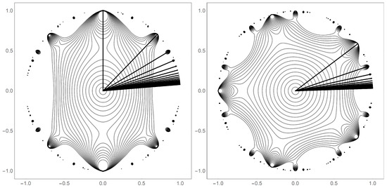
Figure 1.
Two examples of centered polygonal lacunary functions, plotted for , where (see Equation (3)). The left panel shows the case for while the right shows the case of . The superimposed line segments represent the symmetry angles ( through ). The terminus of the line segments at the natural boundary sits at a point where does not converge, but the limit value is a bounded -cycle.
All figures, graphs, and numerical results were generated with home-written Mathematica code.
2. Notation and Background Results
Definitions, notation, and some theorems from Reference [18] are briefly collected here for convenience of the reader.
2.1. Lacunary Sequences and Lacunary Functions
For this work, lacunary sequences of functions are considered. The Nth member of the sequence is given by
where is a function of n satisfying the conditions of Hadamard’s gap theorem [1]. (Note that the sum starts at .) Following Reference [18], the notation
is used to represent the particular lacunary sequence described by , in complex variable z. For example, . The lacunary function associated with the sequence is .
Lacunary sequences of numbers are obtained by identifying a particular value of z. For , the sequences are convergent and not very interesting because is analytic inside the unit disk. Interesting sequences occur when . In general, these sequences are not convergent, but bounded cyclic sequences occur along with divergent sequences. The p-sequences, which arise when is a centered polygonal number, are one such family of bounded cyclic sequences.
2.2. Centered Polygonal and Triangular Numbers
It has been shown that the whole family of centered polygonal lacunary sequences can be consider at once because of the relationship between the centered polygonal numbers (cpns) and the triangular numbers [18].
Centered polygonal numbers are an increasing sequence of numbers arising from considering points on a polygonal lattice [19]. These numbers were discussed in the context of two-dimensional crystal structures by Teo and Sloane [20]. The formula for the centered k-gonal numbers is
The central focus of this work is . The notation is used to denote the mth member of the set.
It turns out that nearly all of the structural features discussed in this work are independent of the choice of k [18]. This is precisely because the cpns are related to the triangular numbers [21], , in a simple way. The notation is used to denote the mth member of the set. For convenience, a lemma proved in Reference [18] is stated here without proof:
Lemma 1.
It is noted that, in work unconnected to the cpns, Atanasov et al., employed the use of a lacunary function based on the triangular numbers in their study of representations of integers as sums of triangular numbers [22]. Additionally, there is a relationship between the triangular number based lacunary functions and mock theta functions [17].
Because of Lemma 1, one can learn much about the entire family of centered polygonal lacunary sequences at once by considering the triangular numbers. Most notably for this work, one is interested in the behavior of the triangular numbers modulo n. While many properties are known about this, there does not appear to be a centralized reference in the literature. The proofs for the following two lemmas and three theorems can be found in Reference [23].
Lemma 2.
The sequence of triangular numbers mod p is a -cycle. The sequence is symmetric about the midpoint of the -cycle. The th member of the -cycle is zero.
Lemma 3.
There is an equal number of even and odd numbers in the first p members of -cycle of Lemma 2.
Theorem 1.
All values appear once and only once in the first p members of the -cycle if and only if where m is a positive integer.
Theorem 2.
If , then the first time 0 appears is at a position less than the position. The converse is also true.
Theorem 3.
Values appear no more than twice in the first p members of the -cycle for p prime.
2.3. p-Sequences
Lemma 1 connects the triangular numbers to the p-sequence of limit values of at the natural boundary along the set of pth symmetry angles. The pth symmetry angle is . The Nth member, , of the p-sequence is part of a -cycle of values. The -cycle reduces to a -cycle when considering rather than . A factor of is the only factor that carries k dependence and is present in every term. Hence, . The sequence of has its own structure as it follows a -cycle. The index of that -cycle is and represents under the mod. This yields a structure for the of the form . Consequently, only p, rather than , distinct must be determined. A very simple expression for the values exists [18]:
where . Note: is really but it proves convenient to limit the run of i to p and define . One collects the as elements of the set , which is called the base space symmetry angle set [18].
2.4. Fiber Bundle Representation of Centered Polygonal Lacunary Sequences
The use of a primitive fiber bundle is a convenient way to deal with the emerging -cycles discussed above and was a main topic of Reference [18]. The reader is alerted, by the use of the word “primitive”, to the fact that this bundle lacks a manifold structure which is attendant when one typically thinks of a fiber bundle [24]. For the convenience of the reader, the primitive fiber bundle machinery is briefly outlined here. A more thorough discussion along with illustrative examples is given in Reference [18].
The base space is the unit circle in the complex plane, . This is not the same complex plane that serves as the domain of the . In the above defined base space, the symmetry angle set is identified: . The set of positive integers, , are the typical fibers which are attached to the base space at the points . The bundle is , where is the total space, and is the projection from to such that maps to the typical fiber and where is , the multiplier set [18]. A cross-section on is a graphical way to represent for a particular N. The collection of all cross-sections on then represent the entire lacunary sequence for . The set of cross-sections for a given value of p can be reduced to the consideration of a single fiber position diagram which is simply a graphical representation of the base space, [18]. (They are not mathematical graphs, however.) is partitioned evenly at every which represents the points on where the fibers are attached. Fiber position diagrams are discussed thoroughly in Reference [18] where the proof of the following theorem can be found.
Theorem 4.
Fiber position diagrams are at least two-fold rotationally symmetric.
3. Construction of Two-Dimensional Base Space Graphs
This section contains two distinct constructions of the two-dimensional base space graphs. “Graph” is meant in the graph theory sense with the added sense that the relative position of the vertices in the plane carry meaning. A concrete example of the construction procedure is carried out for the case. Finally, information that one is able to glean from the graphs is discussed.
3.1. The Construction of the Two-Dimensional Base Space Graphs
Several definitions are needed prior to laying out the construction procedure.
Definition 1.
Division point set, . The ordered set of equally spaced points on . Point 0, , of that set is at (1,0) ( viewing as embedding in ). The remaining ordered points progress counterclockwise on from vertex 0.
Definition 2.
Antipodal pair. Pairs of points .
Definition 3.
Unit increase progression. Identification of members of an ordered set, Q as , where means . Note the spacing between each identified member increases by one.
Definition 4.
Terminal edge. An edge of a graph connected to only one vertex. Alternatively, an edge that connects a vertex with the “vertex at infinity”.
Definition 5.
Multiplicity set, .
Definition 6.
Saturation, s. , where is the vertex set for the base space graph.
The following scheme is used to construct the two-dimensional base space graphs.
Construction 1.
Two-dimensional base space graph, .
- 1.
- Add division points, , to .
- 2.
- Add a vertex at point 0 on . This is referred to as vertex 0. The antipode to vertex 0 is referred to as vertex π.
- 3.
- Add a terminal edge to vertex 0.
- 4.
- Perform unit increase progression through for iterations. This is done going counterclockwise from vertex 0. This builds the set of vertices, . Each step in the progression creates an edge that terminates to either a new or an existing vertex and builds the set of edges, .
- 5.
- Add a terminal edge to vertex π. This completes the graph.
Figure 2 collects the two-dimensional base space graphs for to .
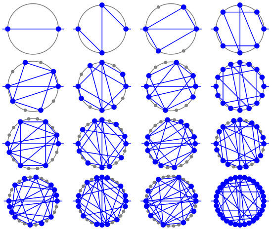
Figure 2.
Two-dimensional base space graphs for through (read left to right, top to bottom). The grey circle represents and small grey dots (sometimes obscured by larger blue dots) represent equally spaced positions . The graph, , is shown in blue. The vertices of the graphs represent terms of the form , . The edges (blue lines) represent steps in the unit increase progression (Definition 3).
3.2. Information Carried in Base Space Graphs
Several straightforward but fundamental observations are expressed in the following lemmas and conjectures.
Lemma 4.
If is a vertex, then so is its antipodal partner, .
Proof.
The proof follows from Lemma 2. □
Lemma 5.
The positions of the antipodal pairs of vertices on a two-dimensional base space graph are equal to the numerical values of . The degree of a vertex is equal to the number of times the corresponding numerical value of appears.
Proof.
The proof follows immediately from Construction 1. □
Theorem 5.
Only one antipodal pair shares an edge. For p odd, this edge connects the 0 and π vertices. For p even, this connects the and vertices.
Proof.
The first part follows immediately from the nature of Construction 1. For an edge to connect antipodes it must count exactly p members of beyond the current vertex. Further, this particular edge is generated by the pth step. The second part follows from Lemmas 2 and 5 once one notes the following. Consider the pth member of T,
Now, considering this expression mod p yields,
If p is even the value of p/2 corresponds to the position of the vertex by Lemma 5. When p is odd this value of p/2 must be zero otherwise it is not an integer. Hence, the position corresponds to the 0-vertex. This completes the proof. □
Lemma 6.
The positions of the vertices on a two-dimensional base space graph give the fiber position diagram.
Proof.
Removal of the edges in the graph leaves the fiber position diagram for the triangular numbers case. Shifting by gives the fiber position diagram for the kth cpn case [18]. □
In providing position information, the two-dimensional base space graphs gives the terms involved in the numerical value of a particular member of a p-sequence. Furthermore, these graphs carry multiplicity information as shown in the following theorem.
Theorem 6.
The degree of a vertex is twice the multiplicity of the term it represents.
Proof.
The proof follows from Construction 1 because each iteration in the construction either:
- creates a new vertex, in which case a new term is represented; or
- lands on an existing vertex, in which case represents a degeneracy (multiplicity) of a term that already exists.
Each pair of subsequent iterative steps creates edges, and . Thus, the vertex linking these edges increases in degree by 2. (The terminal edges ensure this is also true for the 0 and vertices.) This completes the proof. □
The base cross-section can be obtained immediately from the two-dimensional base space diagrams by pulling the information about the fiber positions and the multiplicities. When combined with the cross-section generation procedure thoroughly discussed in Reference [18], one can generate the entire p-sequence from the single two-dimensional base space diagram.
As an illustrative example, consider the case. is the third graph in the top row of Figure 2. One sees that there are four distinct vertices in and positioned at . The base cross-section is obtained by removing the edges of the graphs and casting as the line and reading the multiplicity from (1/2 the degree of each vertex). In this case, the vertices located at and have degree 4 (hence, multiplicity 2), while the vertices located at and have degree 2. The base cross-section is shown as the first fiber diagram in the top row of Figure 3. The unit increases progression and then generates the remaining cross-sections, as shown in Figure 3. Each of these cross-sections corresponds to a numerical value in the associated p-sequence. For the case of , which is the lacunary function on the right in Figure 1, the numerical values are . This list of numerical values corresponds directly to the cross-sections shown in Figure 3 when read left-to-right, top-to-bottom. Note that upon taking the modulus the -cycle reduces to a -cycle. When one factors out the k-dependent common multiplier, the cyclic sequence of values is .
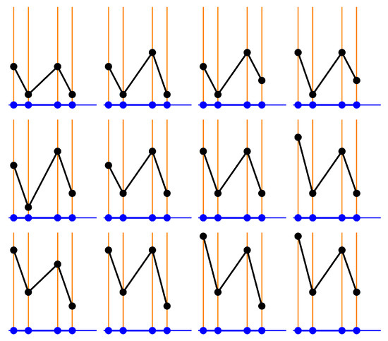
Figure 3.
The complete set of cross-sections for the case of (corresponding to the third graph in the top row of Figure 2). The leftmost cross-section is considered the base cross-section and is obtained directly from . The complete set of cross-sections is obtained from the base cross-section via unit increase progression starting on the first fiber to the right of the midpoint. Each cross-section directly gives the numerical values in the centered polygonal lacunary sequence at the position on the natural boundary at angle .
3.3. Rectangular Construction for Odd p
There is an alternative construction for the two-dimensional base space graphs corresponding to odd values of p. This is called the rectangular construction.
Construction 2.
Rectangular construction (odd p only).
- 1.
- Add division points to .
- 2.
- Add the 0 and π vertices and connecting edge. This is referred to as the 0-rectangle.
- 3.
- Simultaneously perform the first iteration of the unit increase progression counterclockwise from the 0 vertex and from the π vertex.
- 4.
- Add connecting edges from vertex to vertex π and to vertex 0. This forms the 1-rectangle.
- 5.
- The next iterations of the unit increase progression forms the 2-rectangle, etc. The number of iterations of the unit step progression is . The final rectangle formed is called themaximal rectangle.
- 6.
- Add a terminal edge to vertices 0 and π. This completes the graph.
The rectangle construction offers a geometric proof of the following theorem.
Theorem 7.
There are total vertices for graphs of odd prime numbers.
Proof.
The rectangle construction implies that there are total rectangles (including the 0-rectangle) coming from that same number of iterations during the construction process. Further, the top half-circle and the bottom-half circle behave symmetrically because antipodal pairs are arising simultaneously (unlike for Construction 1). Because p is prime, the first iteration step to cross from the top half circle to bottom half-circle (if there is one) produces a new vertex. Consequently, its antipode in top half-circle is also a new vertex and one can base the next iteration step on this vertex. Again, because p is prime, the remaining steps will all create new vertices. Note, this is related to the fact that is a field when p is prime and hence has no non-zero divisors. □
Theorem 7 leads to several corollaries which are listed now without proof.
Corollary 8.
The maximum degree of any vertex is 4 for odd primes (maximum multiplicity is 2).
Corollary 9.
The maximal rectangle has one pair opposing vertices with degree two. All other vertices are degree 4.
Corollary 10.
The saturation of prime graphs are .
4. Three-Dimensional Base Space Graphs
The two-dimensional base space graphs provide much insight in to the centered polygonal lacunary p-sequences and even form the basis for complete construction of the numerical p-sequences themselves. However, at high values of p, the benefits of a visual representation diminish because the graphs become so crowded.
By opening up the used of a third dimension, one is able to obtain a different visual perspective on the graphs. This perspective actually works better at high p values so it is quite complementary to the two-dimensional graphs. The construction procedure for these graphs is the following.
Construction 3.
Three-dimensional base space graphs, .
- 1.
- Create a lattice on the cylinder using and the positive integers.
- 2.
- Create the three-dimensional graph from the corresponding two-dimensional graph by placing the jth vertex at its corresponding division point and value equal to half of its degree (equal to ).
- 3.
- Add a terminal edge to vertex 0 and π (usually not shown in a rendering of the graph). This completes the graph.
Figure 4 shows the three-dimensional base space graphs corresponding to the 16 two-dimensional base space graphs shown in Figure 2. Table 1 collects some information for several important classes of p values. Figure 5 shows four representative examples from Table 1 involving larger values of p.
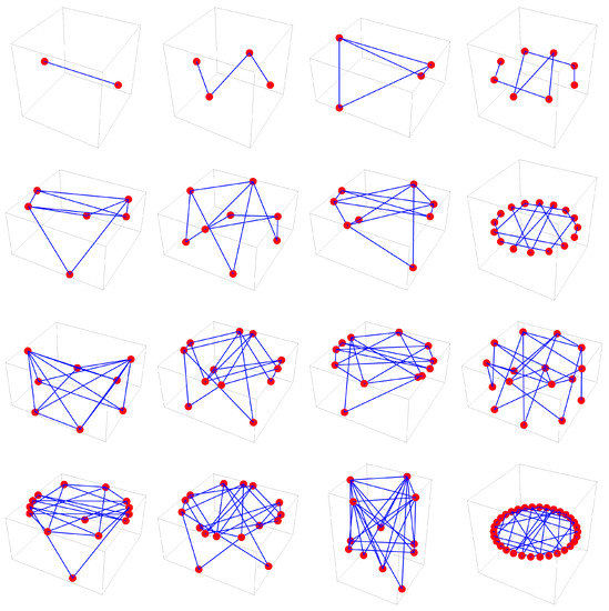
Figure 4.
Three-dimensional base space graphs for to (read left to right, top to bottom). These correspond directly to the graphs in Figure 2, now with the third dimension being the degree of the vertex. In addition to offering a different visual perspective of the p-sequences, the degrees of the vertices within a given graph are intimately related to the nature of p itself and to the values of the centered polygonal lacunary functions at the natural boundary (see text for discussion).

Table 1.
Characteristics of some important types of three-dimensional base space graphs.
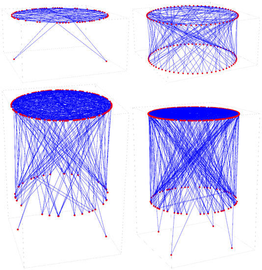
Figure 5.
Three-dimensional base space graphs: (top left); (top right); (bottom left); and (bottom right).
The three-dimensional base space graphs are useful for visually categorizing various families of p values based on their descriptive three-dimensional shape, such as those listed in Table 1. This is especially useful for large p values compared to the two-dimensional version of the graphs. Despite this, the subtle details are less evident. It is helpful to associate with each three-dimensional base space graph and “exploded” version in which the layers are arrayed and the edges removed. The example of the exploded graph of is shown in Figure 6.
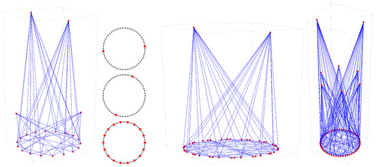
Figure 6.
and corresponding slices (first and second panels), (third panel), and (fourth panel).
5. Prime Decomposition
A powerful feature of the graphs is the insight they provide in understanding the bounded, cyclic nature of the limit values at the natural boundary and pth symmetry angle. In addition to the illuminating graphical characteristics, one can assign a polynomial to each class of three-dimensional base space graph. This polynomial gives the number of vertices contained in the graph and, hence, immediately gives the saturation value upon dividing by . The polynomial for any given graph is constructed via prime polynomials associated with each prime power. These are given in the following construction.
Construction 4.
Base space graph polynomial.
- 1.
- The prime power polynomials are generated via,
- 2.
- Find the prime decomposition of p and let r equal the number of distinct odd primes present in the decomposition.
- 3.
- For a given p, multiply the prime power polynomials represented in the prime decomposition of p and divide by a factor of to obtain the overall polynomial.
- 4.
- Evaluating for a given p gives the number of vertices in .
It is immediate to calculate the saturation of a graph by normalizing the graph polynomial by :
An immediate corollary of Construction 4 and Equation (11) is the following.
Corollary 11.
The saturation is independent of a factor of ,
Consider as an illustrative example. is shown in the left panel of Figure 7. The prime decomposition is . Thus, , , , and . The associated with is
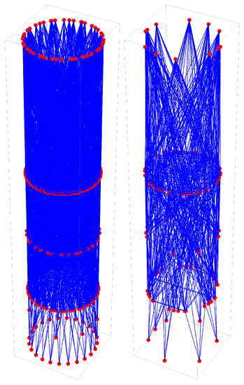
Figure 7.
and . The p values associated with these graphs differ by a factor of and hence have equal saturation values.
The saturation is then immediately
Now, consider the case when which is just 1260 without the factor of . One expects the saturation to be the same as for the and, although not explicitly shown, that is indeed the case.
The Prime Power Family of Graphs
Values of constitute an interesting family. From graphical morphology point-of-view, the most notable feature of this family is that the exploded graph has a nested feature. The structure of the family three-dimensional base space graphs is of the form of an increasing layered crown. For odd powers, this is an layer crown (base layer plus layers of spikes). Furthermore, each progression of n to introduces a new base layer with the spike layers having equivalent vertex positions previous case, albeit with different connectivity. Similar behavior is seen for the even case.
Considering the saturation for the prime power case, one sees approach an asymptotic value with increasing n,
which follows from pulling up the denominator as , distributing through the numerator, recognizing the alternating series and writing it in closed form. Further, as in Equation (15), This behavior is shown in Figure 8. The larger is the value of q, the faster is the convergence to the asymptotic value. By way of example, , which deviates from 3/8 by , whereas and deviate from their respective asymptotic values by and , resoectively.
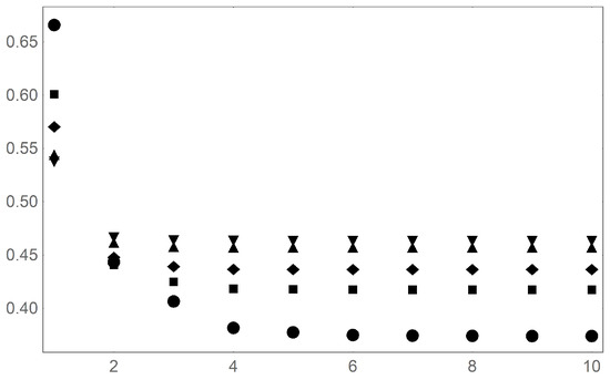
Figure 8.
Behavior of the saturation of prime powers, for (circle); (square); (diamond); (triangle); and ,(inverted triangle). The vertical axis is s and the horizontal axis is m.
The nature of the graph polynomials implies this limit easily extends to products of prime powers.
By Corollary 11, a potential component comes along trivially.
Finally, plotting the entries in the adjacency matrix also provides insight into the nature of the p-sequences. They are especially good at revealing the special nature of primes, prime powers and the scaling properties. The adjacency matrix for a number of different graphs are collected in Figure 9. The top row is meant to visually capture the typical differences between primes and non-primes by showing , , , and . has a particularly “clean” adjacency matrix. The second row shows the squares of the p values used in the top row: , , , and . The differences between primes and non-primes are even more exaggerated. It is also important to note that, for primes, the structure of adjacency matrix is nearly independent the power on the prime. This is seen in comparing and . Aside from picking up some entries along the left and top borders, the adjacency matrix of has the same structure as . The only difference is that it is scaled for the now much larger adjacency matrix. This is also shown in the third row where powers of 5 are used as the example. Here, , , , and are shown. The adjacency matrix for (not shown) is too small to display the characteristic structure seen with . The structure begins to emerge with the still small adjacency matrix for . For , , and , the structure is very clearly present. Note, however, that increasing power does introduce some additional patterning in the adjacency matrix. What is perhaps even more surprising than the scaling insensitivity of the adjacency matrix with prime power, is the scaling insensitivity with respect to choice of the prime itself. Remarkably, aside from scaling, all primes and prime powers look the same.
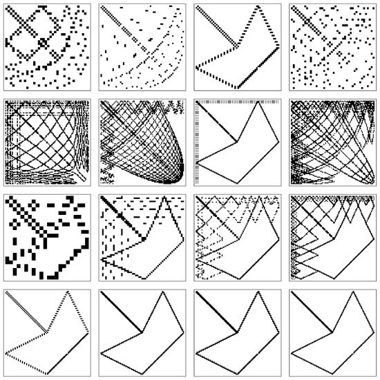
Figure 9.
A plot of the entries of the adjacency matrix for several graphs. The special nature of primes and the inherent scaling properties are particularly noticeable. The top shows the typical differences in the adjacency matrices for primes and non-primes by collecting , , , and . The second row shows , , , and . The third row shows , , , and . The bottom row show several examples of other primes: , , , and .
The above analysis is very helpful in gaining insight into the structure of the saturation data shown in Figure 10. For numbers that are composed of highly redundant primes, the above formula holds. Thus, one expects “attractor” values which are the asymptotic values. Adding in the independence of s from Corollary 4 allows for a good understanding p values of the form . These will be at the same saturation values spaced on the powers of two. Visual inspection of Figure 10 shows clear and distinct striations (or lines of attraction); these are the numbers composed of highly redundant primes. The power of two spacing is also readily seen, for example and several values between roughly and . Thus, there is significant organization of these saturation data.
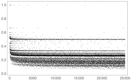
Figure 10.
Saturation values for the first 25,000 integer values of p. Visible striations appear because of the asymptotic “attractor” values of for number whose prime decomposition consist of high redundancy.
The exception occurs for numbers composed of low redundancy primes; most notably the “noisy” data at the low s values. In fact, a noticeable trail of low s values separates slightly from the bulk of the data points. These are the numbers whose prime decomposition consists of first-order primes. Indeed the following conjecture has been verified for the first 32,000 p values, but awaits a general proof.
Conjecture 12.
For a set value, , the p value having the minimum saturation is such that .
6. Antipodal Condensed Graphs
In the use of the base space graphs to understand p-sequences, the vertices sitting at antipodal points in the two-dimensional base space graph have a natural relationship [18]. This suggests a related graph construction called antipodal condensed graphs in which each antipodal vertex pair from the two-dimensional base space graph is merged into a single vertex in the antipodal condensed graph. Notationally, denotes the antipodal condensed graph associated with . has half the number of vertices as .
Construction 5.
Antipodal condensed graph,
- 1.
- Identify all antipodal pairs as .
- 2.
- The collections of edges, , that connect to are identified as a single edge, .
- 3.
- The terminal edges are viewed as connecting vertex 0 with vertex π via the “vertex at infinity”. This collapses to a self-loop . This completes the construction.
Some self-evident aspects of are for even (this includes the self-loops), for odd (includes self-loop), and , where is the degree of vertex (counting self-loops).
As an illustrative example, is shown in Figure 11. The first panel shows the standard embedding whereas the middle panel shows a different rendering (the default rendering used by Mathematica). Note the double edge connecting the two left most vertices in this rendering is an artifact of the terminal edges in the construction. This can be viewed in the following way. One edge connects the two vertices (as in the corresponding base space graph) while the other edge connects the two vertices via the “vertex at infinity”. The right panel shows the corresponding antipodal condensed graph, .
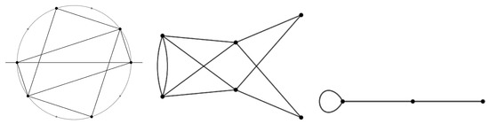
Figure 11.
Renderings of . The left panel is the two-dimensional base space graph. The grey dots represent the members of that are not vertices. The grey circle simple guides the eye to the embedding space, . The middle panel is a different representation of the graph that vertically juxtaposes antipodal vertices. The right rendering is a reduction of the graph by associating antipodal points together as a single vertex. The resulting graphs is . This always reduces the number of vertices by half.
Self-loops occur in the antipodal condensed graph because of the edge connecting antipodal pairs in the base space graph. By Theorem 5, this occurs only at vertex 0 for odd values of p odd and at vertex for even values of p. Note that for even values of p there are actually two self-loops in graphs arising form even values of p, a “real” one which is at vertex and a “virtual” one at vertex 0. (For odd values of p, the self-loop at vertex 0 is real.) The virtual self-loop, seen in the graph is an artifact of the the terminal edges in the base space graph. Again, this can be viewed as an edge connecting a the vertex with itself via the “vertex at infinity”. These self-loops are of no mathematical consequence but, nonetheless, are sometimes helpful in orienting the eye so they are kept in the rendering.
The antipodal condensed graphs for –16 are collected in Figure 12, which correspond directly to the base space graphs shown in Figure 2 and Figure 4. While only a small sampling, some generalities in are exposed. Odd primes are always simple linear graphs with vertices and edges not including the single self-loop. Even values of p yield two self-loops because of Theorem 5. The family is always a simple linear graph with vertices and edges not including the two terminal self-loops. Aside from self-loops, for q an odd prime. This relation is further seen in Figure 13 which shows when p is 2 times an odd number (prime or not). The odds from 3 () to 51 () are shown. Primes are clearly distinctive in shape, being very linear in nature for this particular rendering of . The primes and their powers are the subject of the next section.
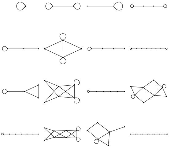
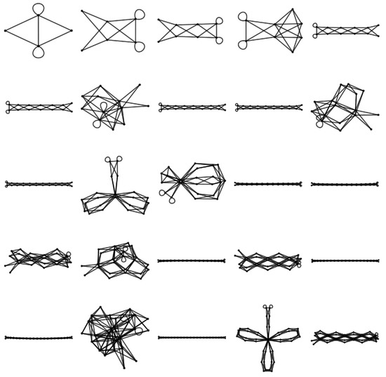
Figure 13.
Antipodal condensed graphs, for for –51 (odds). Graphs corresponding to times a prime are distinctively linearly in shape. Those corresponding to times a prime square also hold their distinctive flower shape.
The nested nature of the primes is evident in the antipodal condensed graphs for even values of p that are powers of two times a prime. For a given power of two, contains as a subgraph where is the prime immediately preceding q. This is illustrated in Figure 14. At first glance this appears to be very exciting because it suggests a mechanism to predict the next prime from a given prime. Unfortunately, this is not the case. For example, the transition from to . Indeed, is a subgraph of , but the predictive power is lost because, in this example, there would be nothing, a priori, to prevent the generation of the false prime graph for .
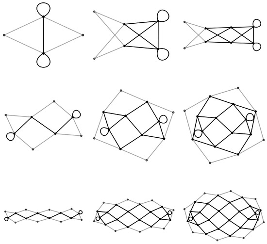
Figure 14.
The nested nature of the primes. for (top row), (middle row) and (bottom row) where . In each case, the graph for a prime has a subgraph equal to the previous prime. This continues for higher primes.
The above discussion along with Figure 13 and Figure 14 suggest an interesting effect of multiplying by a factor of 2. Indeed, such action has the effect of “twining” each vertex. Figure 15 illustrates the “twining” effect caused by multiplying by 2. is compared to . In this example, and . That the number of vertices doubles while the number of edges quadruples results in more cross-linking of vertices. Nevertheless, the twin vertices do not share an edge.
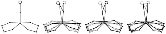
Figure 15.
Illustration of the twining of vertices that results when p is multiplied by 2. is compared to The middle two panels show the two copies of contained in . The last panel shows the remaining edges. Twin vertices do not share an edge.
6.1. Primes
The use the of antipodal condensed graphs obscures the prime decomposition compared with the base space graphs. However, it nicely characterizes the behavior of powers of primes. Some of those characteristics are explored in this section.
6.2. Powers of Primes
Starting with squares of primes, Figure 16 shows where for the first 12 primes. The vernacular of flowers will be used as descriptor. Each square prime forms a flower with petals and one stalk. Each petal consists of a closed loop connecting the single ultimate vertex to itself. There are q edges and degree 2 vertices on the paths that form the petal. The stalk consists of a simple path connecting the ultimate vertex with the vertex that contains the single self-loop. This arrangement gives the ultimate vertex a degree equal to q.
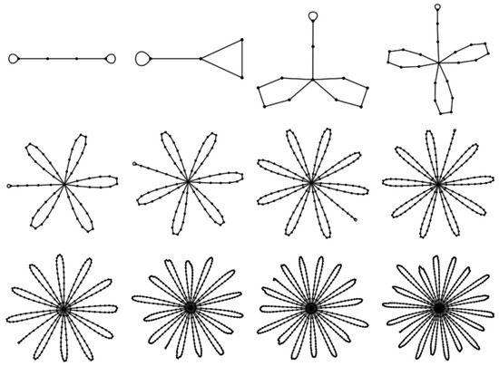
Figure 16.
for p the squares of first 12 primes. The descriptor language for these types of graphs would be that they are -petal flowers.
A example is the family. There are actually two sub-families, one for n odd and one for n even. These antipodal condensed graphs are captured in Figure 17 where along the top row and along the bottom row. Of particular note is the similarity in overall morphology within a subfamily. This is related to the scaling properties of the prime graphs and is discussed in detail below.
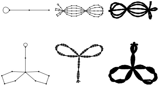
Figure 17.
The family of graphs. The top row shows the n odd subfamily for and the bottom row shows the n even subfamily for .
Finally, in addition to powers of individual primes, there is a “product” graph, for two distinct primes. The descriptor of these product graphs is that of a web. The webbing consists of faces. Exactly one face is triangular and the remaining faces are quadrilaterals. A “multiplication” table involving the first five odd primes is shown in Figure 18. Notice the diagonals recover the flower graph associated with the primes squared. The off-diagonals are webs with faces as described above. Expressing the above in a more pictorial sense, the number of faces equals the product of the number of petals on the respective flowers. The product is, of course, commutative so the upper and lower triangles of the table are identical. The example of is shown in the right panel with the faces labeled. In this case, one expects faces.
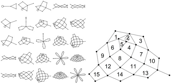
Figure 18.
A graph multiplication table for the first five odd primes, , where . The “product” is a web graph with faces (). The faces consist of one triangle and the remainder are quadrilaterals. The example of is shown on the right with the faces labeled.
7. Scaling Properties
The above discussion strongly implicates the prime powers in the scaling features of centered polygonal lacunary sequences. This is investigated further in this section. First, however, the important new concept of sprays is introduced.
7.1. Sprays
The study of the scaling properties of the centered polygonal lacunary graphs is aided by the introduction of the concept of a spray. (It is trusted that the use of the word spray in this context is distinct enough to avoid confusion with its definition of a particular type of vector field on a tangent bundle [25], to which there is no relation here.)
Definition 7.
Spray. A set of simple linear paths between two primary vertices. The distinct paths are otherwise identical. That is, they have the same number of intermediate vertices and edges and the degree of the intermediate vertices is exactly 2. The paths of a first-order spray do not share a vertex. A second-order spray can be thought of as a spray of first-order sprays; jth-order sprays are sprays of th-order sprays.
Examples of sprays can be seen in several of the figures. In particular, Figure 19 and Figure 20 highlight the notion of a spray. The example of is shown in Figure 19 where the panel on the left shows the entire graph, while the panel on the right shows a blow-up of the right petal and ultimate vertex. One notices five first-order sprays connecting the ultimate vertex to the the adjacent penultimate vertices. There are five first-order sprays terminating with the ultimate vertex. Each penultimate vertex terminates two sprays.
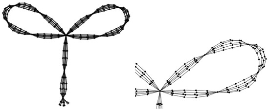
Figure 19.
illustrates the concept of spray. The left panel shows the entire graph while the right panel is a blow-up of one of the petals. Five first-order sprays are connected to the ultimate vertex and each penultimate vertex is terminated by two sprays. Because , the first-order sprays have five paths each and each path consists of five edges and four intermediate degree 3 vertices. Application of the renormalization scheme discussed in the text would yield , which is shown in Figure 17.
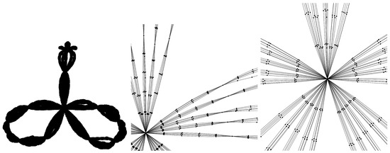
Figure 20.
is an example of a graph with second-order sprays. The left panel shows the entire graph while the middle and right panels are blow-ups of the area around the ultimate vertex. Five second-order sprays are connected to the ultimate vertex and each member of the spray is itself a (first-order) spray. Twenty-five first-order sprays connect the ultimate vertex to an antepenultimate vertex. These 25 first-order sprays are organized into five second-order sprays, each of which connects the ultimate vertex to the the penultimate vertex. Because , the first-order sprays have five paths each and each path consists of five edges and four intermediate degree 3 vertices while the second-order sprays have five paths of first-order sprays. One iteration of the renormalization scheme discussed in the text would yield which is shown in Figure 19. A second iteration of the renormalization scheme would yield , which is shown in Figure 17.
There are additional features of note. The graph contains two petals and a stalk, as described above, connecting at the one ultimate vertex. Each petal contains four penultimate vertices while the stalk contains two. Every path in every spray has four degrees and two vertices and every spray contains five paths. All these features generalize such that, for a prime number, q, there are petals and one stalk. Each petal contains penultimate vertices and there are q paths with degree 2 vertices in every spray.
Figure 20 shows as a concrete example of a graph containing a second-order spray. The left panel shows the entire graph. Unfortunately, the large number of vertices obscures the details of the connectivity. The middle panel shows a blow-up the ultimate vertex. There are 25 first-order spays connecting the ultimate vertex with adjacent antepenultimate vertex. These 25 first-order sprays are clustered into five second-order sprays, which connect the ultimate vertex with the five adjacent penultimate vertices. Similar to above, the case of is representative of general features. At the level, there are the same number of petals and stalks. Each petal contains penultimate vertices. In between each of these are antepenultimate vertices and in between those are degree 2 vertices. All second-order sprays contain first-order sprays.
One continues the above analysis for in the obvious way. The same general features occur for the cases of ; again in the obvious way.
7.2. Sprays, Renormalization, and Fractal Character
Sprays provide a natural renormalization scheme for prime power graphs. If the first-order sprays in are replaced by edges the graph reduces to . In this process, second-order sprays become first-order sprays. Likewise, jth-order sprays become th-order sprays. This process can be repeating until is fully reduce to when j is odd and when j is even.
Perhaps more importantly, the reverse of the renormalization scheme can be performed. Here, each edge is replaced with a spray of q paths; each path having q edges. In a sense this acts to “fractalize” the graph. Consider again Figure 16, Figure 19, and Figure 20. The third graph in the top row of Figure 16 is . Considering the ultimate vertex and comparing with Figure 19 one sees the five edges become five groups of five. Then, comparing with Figure 20, one sees 125 edges grouped in the five groups of five, which are further grouped into five. The other vertices behave similarly. Thus, the act of raising the power on the prime is akin to zooming in on a fractal object. Relatedly, the actual fractal character as manifested by Julia sets for the centered polygonal lacunary functions has recently been investigated [26].
Several basic properties of antipodal condensed graphs of prime powers can be immediately gleaned from their scaling structure.
Conjecture 13.
The graph diameter,
Conjecture 14.
The graph radius . This does not hold when n is odd and .
A couple of definitions related to diameter and radius are useful for the even prime powers which have the flower graph structure. In those cases, there is a single ultimate vertex. One then defines the following.
Definition 8.
Ultimate distance, u. The distance from a vertex from the ultimate vertex.
Definition 9.
Ultimate radius, . The maximum distance from the ultimate vertex for a graph.
Conjecture 15.
Finally, an observation awaiting proof is reported: is linearly related to the mean distance for for and prime. For , the relationship is .
8. Graph Theoretic Properties
Several graph theoretic properties are collected in this section. In addition, the concept of a cycle spectrum is developed. The purpose of this section is to provide some unproven conjectures and proposition that are supported by observation. It is hoped that they will offer some potential graph theoretic directions for future work.
8.1. Cliques and Chromatic Number
The antipodal condensed graphs have relatively simple clique structure, which is summarized in a couple of conjectures and propositions.
Conjecture 16.
The maximum cliques always includes vertex 0 or vertex . At least one member of the set of maximum cliques includes vertex 0 (vertex ).
Proposition 17.
Formula for the clique number. The clique number is is 1 plus the number of distinct primes in the prime decomposition of p (this includes 2). The exception is when , then . If 2 is not one of the distinct primes then there is a unique maximum clique. If one factor of 2 is present then there are maximal cliques where r is the number of distinct odd prime factors. Finally, if more than one factor of 2 is present then there are two maximal cliques.
Figure 21 shows the complete graphs isomorphic to the cliques corresponding to Theorem 17. Figure 22 explores the set . The p values all consist of three distinct primes; hence, by Theorem 17, we see the maximum cliques are complete graphs of 4 vertices (plus self-loops). The set of maximum cliques are of size 4 for and (2 to the first power). Further, vertex 0 and vertex are both contained in each clique. There are only two maximal cliques for (2 to an even power), one containing vertex 0 and the other containing vertex .
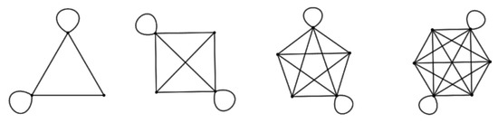
Figure 21.
Maximum clique subgraphs for the cases of p equals two, three, four, and five distinct primes. The maximum clique subgraph is unique.
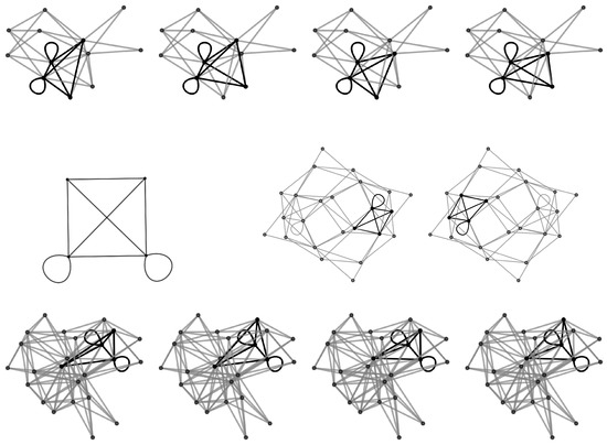
Figure 22.
Maximum cliques for: (top row); (middle row); and (bottom row). The left panel in the middle row shows the complete graph isomorphic to the maximal cliques in this set of graphs. Note that the isomorphism is up to the self-loops.
As with the cliques, the chromatic number is relatively simple. One note, however, is that the graphs must be considered without the self-loops in order for the chromatic number to make sense.
Conjecture 18.
if and only if p is a prime or a power of 2 and there are exactly two ways to color the graph.
8.2. Cycles and the Cycle Spectrum
One can examine the nature of the cycles appearing in the graphs. This can be done by calculating a normalized cycle spectrum, which counts the number of different cycle lengths present in a given graph normalized by the largest value. Several normalized cycle spectra are shown in Figure 23 and Figure 24. In the former case, the normalized cycle spectra for graphs, for , , and where q is an odd prime. Expectedly, when in the first case, 5 in the second case, and 7 in the third case, one sees a single spectral line at q. The cases of are interesting in that they clearly exhibit a self-similarity scaling as can be seen by inspection of the top two rows of Figure 23. In contrast, the cases of and behave more typically. As the value of p increases, the spectrum becomes more Gaussian-like as seen in the bottom three rows of Figure 23. For the cases of graphs in which , again has special character. The top row of Figure 24 shows the normalized cycle spectra for and, indeed, these spectra display a self-similarity and are quite distinct from those shown in the bottom row which are for the cases of .
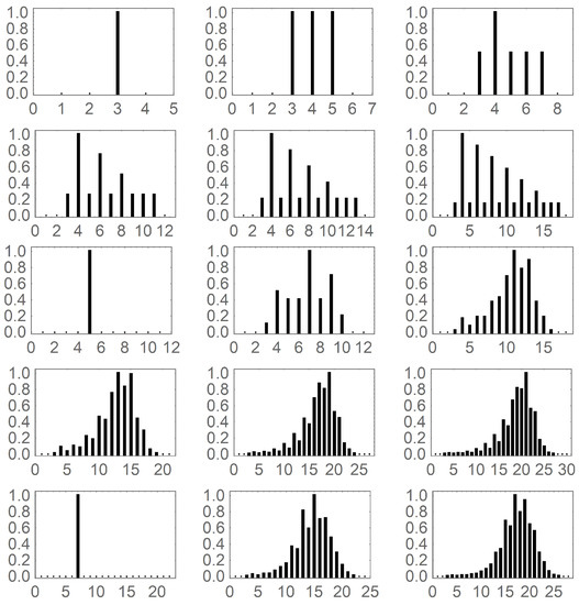
Figure 23.
The normalized cycle spectrum for products of two odd primes. The top two rows are , where . The third and fourth rows are , where . The final row is , where .
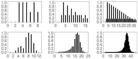
Figure 24.
The normalized cycle spectrum for products of powers of two and one odd prime. The cases of (top row) and (bottom row) where .
9. Conclusions
This work presents a graph-based approach to developing p-sequences of centered polygonal lacunary functions. A ground-up set of construction scheme is shown to build the numerical values in p-sequences. This first involves the two-dimensional base space graphs. This is then followed by the cross-section generating procedure of Reference [18]. Further, an associated three-dimensional graph is developed to provide a complementary view of the p-sequences. The three-dimensional geometric features of these graphs reveal fundamental characteristics of the p-sequences they represent. A polynomial is assigned to each graph, which gives the number of vertices. This allows for immediate calculation of the saturation. Intuitive insights into the structure of the saturation data is provided by use of the polynomials. Additionally, a natural reduction of the base space graphs to an antipodal condensed graph provides much additional insight, especially in regard to the special role of primes. The antipodal condensed graphs are adjoined with the concept of sprays, which enables a clear view of the scaling properties of the underling systems that the graphs represent. Two complementary schemes are discussed: a renormalization scheme, which provides a way to cast in terms of (odd n) or (even n), and a fractalization scheme to build from (odd n) or (even n).
The features of the graphs studied in this work provide much insight into the p-sequences of centered polygonal lacunary functions. This helps one gain an intuition about these exotic and interesting functions.
Notably, the way in which reveals the scaling features of the the graphs and hence the underlying p-sequences that they represent, shines light on the fractal-like characteristics of the centered polygonal lacunary functions. Even more, it provides a possible handle for a potential renormalization scheme for centered polygonal lacunary functions. If such a scheme is found and is robust, then it seem likely that these function could find greater utility in physics and chemistry; the area of phase transitions is one example.
The graph-theoretic analysis done here also indicates some potential ways to bring-out various subsequences that are carried in the centered polygonal lacunary functions. For example, one might be inclined to consider the family of p-sequences consisting only of . Comparison of these families as either or could reveal some interesting results.
It is hoped that this work builds upon previous work and sheds additional light on the the fascinating nature of centered polygonal lacunary functions and, in particular, on their p-sequences. The unproven conjectures are the subject of ongoing research.
Author Contributions
K.S. and D.J.U. conceived the investigation; K.S. and D.J.U. designed the investigation; K.S. and D.J.U. provided background for the investigation; D.J.U. wrote the Mathematica code to perform the investigation; D.R. developed distributed computing capabilities; K.S., D.R. and D.J.U. analyzed the data; K.S. and D.J.U. wrote the original draft of manuscript; and K.S., D.R. and D.J.U. edited the manuscript.
Funding
This research was funded by the Concordia College Chemistry Endowment Fund.
Acknowledgments
We thank Douglas R. Anderson, Leah Mork, and Trenton Vogt for valuable discussion.
Conflicts of Interest
The authors declare no conflict of interest. The funders had no role in the design of the study; in the collection, analyses, or interpretation of data; in the writing of the manuscript, or in the decision to publish the results.
References
- Hille, E. Analytic Function Theory Vol. II; Ginn and Company: Boston, MA, USA, 1962. [Google Scholar]
- Kahane, J.-P. A century of interplay between Taylor series, Fourier series and Brownian motion. Bull. Lond. Math. Soc. 1997, 29, 257–279. [Google Scholar] [CrossRef]
- Hille, E. Analytic Function Theory, Vol. I; Ginn and Company: Boston, MA, USA, 1959. [Google Scholar]
- Creagh, S.C.; White, M.M. Evanescent escape from the dielectric ellipse. J. Phys. A 2010, 43, 465102. [Google Scholar] [CrossRef]
- Greene, J.M.; Percival, I.C. Hamiltonian maps in the complex plane. Physica D 1981, 3, 530–548. [Google Scholar] [CrossRef][Green Version]
- Shudo, A.; Ikeda, K.S. Tunneling effect and the natural boundary of invariant tori. Phys. Rev. Lett. 2012, 109, 154102. [Google Scholar] [CrossRef] [PubMed]
- Guttmann, A.J.; Enting, I.G. Solvability of some statistical mechanical systems. Phys. Rev. Lett. 1996, 76, 344–347. [Google Scholar] [CrossRef]
- Orrick, W.P.; Nickel, B.G.; Guttmann, A.J.; Perk, J.H.H. Critical behavior of the two-dimensional Ising susceptibility. Phys. Rev. Lett. 2001, 86, 4120–4123. [Google Scholar] [CrossRef] [PubMed]
- Nickel, B. On the singularity structure of the 2D Ising model susceptibility. J. Phys. A Math. Gen. 1999, 32, 3889–3906. [Google Scholar] [CrossRef]
- Yamada, H.S.; Ikeda, K.S. Analyticity of quantum states in one-dimensional tight-binding model. Eur. Phys. J. B 2014, 87, 208. [Google Scholar] [CrossRef]
- Jensen, G.; Pommerenke, C.; Ramirez, J.M. On the path properties of a lacunary power series. Proc. Am. Math. Soc. 2014, 142, 1591–1606. [Google Scholar] [CrossRef]
- Aistleitner, C.; Berkes, I. On the central limit theorems for f(nkx). Probab. Theory Relat. Fields 2010, 146, 267–289. [Google Scholar] [CrossRef]
- Fukuyama, K.; Takahashi, S. The central limit theorem for lacunary series. Proc. Am. Math. Soc. 1999, 127, 599–608. [Google Scholar] [CrossRef]
- Salem, P.; Zygmund, A. On lacunary trigonometric series. Proc. Natl. Acad. Sci. USA 1947, 33, 333–338. [Google Scholar] [CrossRef] [PubMed]
- Blendeck, T.; Michaliček, J. L1-norm estimates of character sums defined in a Sidom set in the dual of a Kac algebra. J. Oper. Theory 2013, 70, 375–399. [Google Scholar] [CrossRef]
- Wang, S. Lacunary Fourier series for compact quantum groups. Commun. Math. Phys. 2017, 349, 895–945. [Google Scholar] [CrossRef]
- Lovejoy, J. Lacunary partition functions. Math. Res. Lett. 2002, 9, 191–198. [Google Scholar] [CrossRef]
- Rutherford, D.; Sullivan, K.; Ulness, D.J. Centered Polygonal Lacunary Sequences. Mathematics 2019, 7, 943. [Google Scholar]
- Schlicker, S.J. Numbers simultaneously polygonal and centered polygonal. Math. Mag. 2011, 84, 339–350. [Google Scholar] [CrossRef]
- Teo, B.K.; Sloane, J.A. Magic numbers in polygonal clusters. Inorg. Chem. 1985, 24, 4545–4558. [Google Scholar] [CrossRef]
- Hoggatt, V.E., Jr.; Bicknell, M. Triangular numbers. Fibonacci Q. 1974, 12, 221–230. [Google Scholar]
- Atanasov, A.; Bellovin, R.; Loughman-Pawelko, I.; Peskin, L.; Potash, E. An asymptotic for the representation of integers as sums of triangular numbers. Involve 2008, 1, 111–121. [Google Scholar] [CrossRef][Green Version]
- Structure and Properties of the Triangular Numbers Modulo m. Available online: www.researchgate.net/publication/334389220Structureandpropertiesofthetriangular numbersmodulom (accessed on 11 July 2019).
- Steenrod, N. The Topology of Fibre Bundles; Princeton University Press: Princeton, NJ, USA, 1950. [Google Scholar]
- Poor, W.A. Differential Geometric Structures; Dover: Mineola, NY, USA, 2007. [Google Scholar]
- Mork, L.K.; Vogt, T.; Sullivan, K.; Rutherford, D.; Ulness, D.J. Exploration of filled-In Julia sets arising from centered polygonal lacunary functions. Fractal Fract. 2019, 3, 42. [Google Scholar] [CrossRef]
© 2019 by the authors. Licensee MDPI, Basel, Switzerland. This article is an open access article distributed under the terms and conditions of the Creative Commons Attribution (CC BY) license (http://creativecommons.org/licenses/by/4.0/).