Article

On the Integral of the Fractional Brownian Motion and Some Pseudo-Fractional Gaussian Processes

1
Dipartimento di Matematica, Università “Tor Vergata”, 00133 Rome, Italy
2
Dipartimento di Matematica e Applicazioni, Università “Federico II”, Complesso Monte S. Angelo, 80126 Napoli, Italy
*
Author to whom correspondence should be addressed.
Mathematics 2019, 7(10), 991; https://doi.org/10.3390/math7100991
Submission received: 28 June 2019 / Revised: 28 September 2019 / Accepted: 16 October 2019 / Published: 18 October 2019
(This article belongs to the Special Issue Stochastic Processes in Neuronal Modeling)

Abstract

:
We investigate the main statistical parameters of the integral over time of the fractional Brownian motion and of a kind of pseudo-fractional Gaussian process, obtained as a classical Gauss–Markov process from Doob representation by replacing Brownian motion with fractional Brownian motion. Possible applications in the context of neuronal models are highlighted. A fractional Ornstein–Uhlenbeck process is considered and relations with the integral of the pseudo-fractional Gaussian process are provided.

1. Introduction

In the last two decades, an increasing amount of attention has been dedicated to non-Markov stochastic processes [1,2]. This happened in many application fields, such as that of finance, biology, genetics, neuroscience, and so on (see, for instance, [3,4,5,6]). The motivation is essentially in the need to design more realistic stochastic models, even if mathematically more complicated [7,8]. Such models include memory in the mathematical description, (see, for instance, [9]). More recently, we aimed to give a contribution in this direction and we studied at first some stochastic processes obtained as integrals over time of Gauss–Markov (GM) processes [10,11,12]. Indeed, such processes, while remaining Gaussian, are no longer of Markov-type: they preserve in some way the memory of their own time evolution. More recently, the fractional calculus [13], and its application to the stochastic analysis [14], provides an alternative strategy to include memory in some stochastic models. The main reason is the non-local nature of the fractional operators such as derivatives and integrals. Similarly to what done for integrated GM processes in [11], we then considered the fractional Riemann–Liouville (RL) integral of order α ( 0 , 1 ) of a GM process. In [15], specifically, we studied the qualitative behavior of such integrated processes, as varying the parameter α , that turned out to have a key rule in the determination of how much memory has to be included in the stochastic description.
An additional useful stochastic tool suitable for developing non-Markov models is the fractional Brownian motion (FBM) [16]. This Gaussian process has properties useful for modeling those phenomena whose temporal evolution shows some kind of dependency; indeed, FBM has stationary increments with long-range (short) dependence if its Hurst parameter H ( 0 , 1 ) is greater than 1 / 2 (less than 1 / 2 ). Furthermore, the FBM coincides with the classical Brownian Motion (BM) if H = 1 / 2 .
Here, we consider a new class of stochastic processes that we call pseudo-fractional Gaussian process (pFG), obtained by the classical Doob representation of GM processes by replacing the BM with the FBM. We investigate the integral over time of such kind of pseudo-fractional Gaussian process. With this aim, we firstly study the integral over time of the FBM and investigate its main statistical properties (mean and covariance). We define the latter as the integrated FBM (IFBM).
Note that, while in [15] the fractional RL integral of a GM process was studied, here we deal with its fractional counterpart concerning the noise: precisely, we consider the ordinary Riemann integral, but involving pseudo-fractional GM processes instead of the classical GM ones. In other words, the fractional feature is shifted from the integral operator to the stochastic term that, in the models, is involved as the noise process.
Here, we also show how varying the Hurst index H of the FBM affects the integral of the considered process, and if this can be possibly put into relation with the fractional RL integral of a GM process, already studied in [15].
The wealth of behavior of the integral of these new processes could be useful in the scope of neuronal stochastic models that is a research field in which recently several fractional models have been proposed, (see, e.g., [17,18] and references therein).

1.1. The FBM Process and Its Integral

We recall that FBM B H ( t ) is a continuous-time Gaussian process starting at zero, with zero mean for all t , having the following covariance function:
E ( B H ( s ) B H ( u ) ) = 1 2 ( u 2 H + s 2 H | u s | 2 H ) ,
where H ( 0 , 1 ) is the Hurst index. For H = 1 / 2 , the process becomes the ordinary BM, while, for H = 1 , as follows by (1), one has E ( B 1 ( s ) B 1 ( u ) ) = s u and so B 1 ( t ) = t ξ , where ξ denotes a standard Gaussian random variable. For H > 1 / 2 , the increments of the process turn out to be positively correlated, while for H < 1 / 2 they are negatively correlated (see, e.g., [16]). Moreover, B H ( t ) has the self-similarity property, with parameter of self-similarity (or scaling exponent) H , namely, for any c > 0 , one has B H ( c t ) = d c H B H ( t ) .
FBM B H is the only Gaussian self-similar process with stationary increments, but they are not independent (see, e.g., [19,20]); furthermore, one has the following representation of B H , in terms of BM B t (see, e.g., [21]):
B H ( t ) = 1 Γ ( H + 1 / 2 ) 0 ( ( t s ) H 1 / 2 ( s ) H 1 / 2 ) d B s + 0 t ( t s ) H 1 / 2 d B s ,
where Γ is the Euler’s Gamma function.
Here, we focus our attention on the integral over time of the FBM, i.e.,
I H ( t ) = 0 t B H ( s ) d s
that we call the integrated FBM (IFBM). In particular, we study its statistical property; this is analogous to what done in [15], where we have studied the Riemann–Liouville integral of order α ( 0 , 1 ) of a GM process Y ( t ) , which is
I α ( Y ) ( t ) = 1 Γ ( α ) 0 t ( t s ) α 1 Y ( s ) d s .
Some comparisons between the above processes will be provided.

1.2. Neuronal Models and Pseudo-Fractional Gaussian Processes

To explain how IFBM can be used for neuronal modeling, one can consider, as an application example, the following model based on the coupled differential equations, for t 0 :
V ( t ) = g L C m V L + η ( t ) C m , V ( 0 ) = V 0 , d η ( t ) = ς τ d B H ( t ) , η ( 0 ) = η 0 .
A similar model was considered in [11] with BM, here substituted by FBM B H ( t ) . The above model is a modified version of a classical Integrate-and-Fire (IF) neuronal model in which the stochastic component is classical white noise.
Specifically, V ( t ) represents the voltage of the neuronal membrane, C m is the membrane capacitance, g L the leak conductance, V L the resting (equilibrium) level potential, and τ and ς parameters regulating the correlation of increments of η ( t ) . The initial values V 0 and η 0 can be specified constants or random variables. In this model, it appears evident the rule of the integral over time of an FBM; indeed, the V ( t ) process involves the integral of FBM B H ( t ) that, in the physical interpretation, includes the time evolution of the interaction with the surrounding environment. Properly, we will say that V ( t ) is a simple example of IFG process, being a non-Markov process involving the integral of the FBM.
A slightly modification of model (4) can be one in which a term I ( t ) of external current is added, i.e.,
V ( t ) = g L C m V L + η ( t ) C m , V ( 0 ) = V 0 , d η ( t ) = I ( t ) τ d t + ς τ d B H ( t ) , η ( 0 ) = η 0 ,
or a more complicated one in which a leaky-term is also included, i.e., the following modified Leaky Integrated-and-Fire (LIF) model with a fractional noise:
V ( t ) = g L C m V L + η ( t ) C m , V ( 0 ) = V 0 , d η ( t ) = η ( t ) I ( t ) τ d t + ς τ d B H ( t ) , η ( 0 ) = η 0 .
Thus, according to (4)–(6), V ( t ) can be written in terms of the integral over time of the Gaussian process η ( t ) , namely
V ( t ) = 0 t V ( s ) d s = V 0 + g L C m V L · t + 1 C m 0 t η ( s ) d s ,
while η ( t ) is a process that solves the second equation of models (4), (5) or (6), respectively. In any case, it is possible to say that the solution process V ( t ) involves the integral of an FBM.
We recall that in the classical version of above models, where a BM B ( t ) is in place of the FBM B H ( t ) , the solution process V ( t ) is a GM process. For such kind of processes the following Doob representation is valid, i.e.,
Y ( t ) = m ( t ) + h 2 ( t ) B ( r ( t ) ) , t 0 ,
where m ( t ) , h 1 ( t ) , h 2 ( t ) are continuous functions of t 0 , which are C 1 in ( 0 , + ) and such that h 2 ( t ) 0 , and r ( t ) = h 1 ( t ) / h 2 ( t ) is a non-negative, differentiable function, with r ( t ) > 0 for t > 0 . The GM process Y ( t ) defined in (7) has mean m ( t ) and covariance c ( u , t ) : = c o v ( Y ( u ) , Y ( t ) ) = h 1 ( u ) h 2 ( t ) , 0 u t .
Here, in order to design a wider class of processes that could be suitable to investigate models such as (4), (5) or (6), we consider processes obtained by means of a formula analogous to (7), i.e.,
Y H ( t ) = m ( t ) + h 2 ( t ) B H ( r ( t ) ) ,
with B H ( t ) an FBM with Hurst index H . Indeed, by analogy with the definition (7) of the classical GM process, we will consider the fractional counterpart of it, obtained by replacing in (7) the ordinary BM B ( t ) with FBM B H ( t ) ; the obtained process is Gaussian, but non-Markov, since FBM is not. We call Y H ( t ) pseudo-fractional Gauss (pFG) process.
Notice that we use the term “pseudo-fractional Gaussian”, since “fractional Gaussian” is used usually for self-similar GP, and Y H ( t ) is not self-similar, in general.
In particular, the present contribution is devoted to the study the integral over time of Y H ( t ) , i.e.,
X H ( t ) = 0 t Y H ( s ) d s .
The process Y H ( t ) can be interpreted as the “velocity process” and X H ( t ) as the “position process”, analogous with the Langevin equation describing the velocity of a particle subject to a random motion in a fluid. We call X H ( t ) the IpFG process. We already remarked that the process Y H ( t ) finds interesting applications in several fields (see, e.g., the discussion in [22]). Note that, from (8), Y H ( t ) is written in terms of an FBM in the transformed time r ( t ) . We point also that a different approach was followed in [23], where the time-changed fractional Ornstein–Uhlenbeck process was studied, in which the time change is given by the inverse of a subordinator.
The mean of Y H ( t ) is m ( t ) and, by taking into account (1), its covariance function turns out to be
c o v ( Y H ( u ) , Y H ( t ) ) = 1 2 h 2 ( u ) h 2 ( t ) r ( t ) 2 H + r ( u ) 2 H | r ( t ) r ( u ) | 2 H .
In Section 2, we calculate the mean and the covariance of the IFBM I H ( t ) and of the IpFG X H ( t ) processes, providing some plots and comparing considerations.

1.3. A Fractional Ornstein–Uhlenbeck Process for Some Comparisons

In classical (non fractional) stochastic calculus, it is well known that the OU process Y O U can be constructed as the unique strong solution of the Langevin SDE:
d Y O U ( t ) = μ Y O U ( t ) d t + σ d B t , Y O U ( 0 ) = y ,
where μ , σ > 0 and B t is standard BM, starting from 0 . The solution of (11) can be expressed as
Y O U ( t ) = e μ t y + 0 t σ e μ s d B s .
Moreover, Y O U ( t ) can also be written as:
Y O U ( t ) = d e μ t [ y + B ( r ( t ) ) ] ,
which is the equality is meant in distribution, with
r ( t ) = σ 2 2 μ e 2 μ t 1 .
Thus, the OU process Y O U turns out to be a special case of a continuous GM process because its form (13) is the same as (7) with m ( t ) = e μ t y , h 2 ( t ) = e μ t and r ( t ) as in (14). Now, replacing in (11) the BM with the FBM, the process Z H ( t ) is obtained, and it is called fractional OU (FOU) process of the first kind in [24] (see also [23]), which is solution of the SDE:
d Z H ( t ) = μ Z H ( t ) d t + σ d B H ( t ) .
Similarly to (12), the solution can be expressed as
Z H ( t ) = e μ t z + 0 t σ e μ s d B H ( s ) .
The stochastic integral exists pathwise as a Riemann–Stieltjes integral (see [25]). Although it is not possible to obtain a representation for Z H ( t ) analogous to (13), alternatively, we can consider a pseudo-fractional OU process, defined as:
Y p F O U ( t ) = e μ t [ y + B H ( r ( t ) ) ] ,
where, for the sake of notation simplicity, we drop the dependence of Y p F O U from H , and r ( t ) is given by (14). We use the term “pseudo-fractional OU process”, since Y p F O U ( t ) defined by (17) does not satisfy, in general, the usual properties of the OU process; for instance, the mean reverting property is not guaranteed.
Some comparisons can be done between the above processes. Indeed, for the pseudo-fractional OU process Y p F O U ( t ) , one gets:
m ( t ) = y e μ t
and, from (10),
c H ( u , t ) = 1 2 e μ ( t + u ) σ 2 2 μ 2 H ( e 2 μ t 1 ) 2 H + ( e 2 μ u 1 ) 2 H | e 2 μ t e 2 μ u | 2 H ,
which can be compared with those of Z H ( t ) . Note that, for H = 1 / 2 , one obtains again the variance and covariance of (classical) OU process (11), namely:
v a r ( Y 1 / 2 ( t ) = σ 2 2 μ e 2 μ t ( e 2 μ t 1 ) , c 1 / 2 ( u , t ) = σ 2 2 μ e μ ( t u ) e μ ( t + u ) .
In Section 3, in order to find relations between the FOU and the IFBM, we evaluate the covariance of the fractional OU process Z H ( t ) in terms of the covariance of FBM B H ( t ) and of IFBM I H ( t ) .

2. Integrated Fractional Gaussian Process

We start with studying the integral over time of FBM:
I H ( t ) = 0 t B H ( s ) d s .
Note that I H ( t ) has a self-similarity property with scaling exponent H + 1 , since, for any c > 0 , one has I H ( c t ) = d c H + 1 I H ( t ) . Moreover, I H ( t ) is a Gaussian process, whose variance is:
v a r ( I H ( t ) ) = E 0 t B H ( s ) d s · 0 t B H ( u ) d u = 0 t d s 0 t d u E ( B H ( s ) B H ( u ) ) = 0 t d s 0 t d u 1 2 ( u 2 H + s 2 H | u s | 2 H ) = 0 t d u 0 u d s 1 2 ( u 2 H + s 2 H ( u s ) 2 H ) + 0 t d u u t d s 1 2 ( u 2 H + s 2 H ( s u ) 2 H ) = 2 0 t d u 0 u d s 1 2 ( u 2 H + s 2 H ( u s ) 2 H ) = t 2 H + 2 2 H + 2 .
Note some analogy with the variance of the Riemann–Liouville integral of BM, I α ( B ) ( t ) (see (3) for the definition), for which v a r ( I α ( B ) ( t ) ) = t 2 α + 1 ( 2 α + 1 ) Γ 2 ( α + 1 ) , α ( 0 , 1 ) (see [15]). In fact, for 0 < H < 1 / 2 , taking α = H + 1 / 2 , we get v a r ( I H ( t ) ) = Γ 2 ( H + 3 / 2 ) v a r ( I H + 1 / 2 ( B ) ( t ) ) ; in general, for H ( 0 , 1 ) , we have v a r ( I H ( t ) ) = ( 2 H + 1 ) Γ 2 ( H + 1 ) t 2 H + 2 · v a r ( I H ( B ) ( t ) ) . These equalities for the variances allow for relating the behavior of an integral of FBM B H ( t ) to that of the RL integral of BM B t , when varying the Hurst index H ( 0 , 1 ) .
In Figure 1, we show the shape of the variance v a r ( I H ( t ) ) as a function of t > 0 , for some values of H ( 0 , 1 ) .
For u t , the covariance function of I H ( t ) is:
c o v ( I H ( u ) , I H ( t ) ) = E 0 u B H ( s ) d s 0 t B H ( v ) d v = 0 u d s 0 t d v E ( B H ( s ) B H ( v ) ) = 0 u d s 0 t d v 1 2 v 2 H + s 2 H | v s | 2 H = 0 u d s 0 u d v 1 2 ( v 2 H + s 2 H | v s | 2 H ) + 0 u d s u t d v 1 2 ( v 2 H + s 2 H ( v s ) 2 H ) .
The first double integral is equal to u 2 H + 2 2 H + 2 , because of (19); thus, one gets:
c o v ( I H ( u ) , I H ( t ) ) = u 2 H + 2 2 H + 2 + 1 2 0 u d s u t v 2 H + s 2 H ( v s ) 2 H d v = u 2 H + 2 2 H + 2 + 1 2 ( 2 H + 1 ) u t 2 H + 1 + t u 2 H + 1 + ( t u ) 2 H + 2 2 H + 2 2 u 2 H + 2 t 2 H + 2 u 2 H + 2 2 H + 2 .
Of course, for u = t , one obtains again the expression (19) of the variance of I H ( t ) .
Notice that, for H = 1 / 2 , one has v a r ( I H ( t ) ) = t 3 / 3 , and c o v ( I H ( u ) , I H ( t ) ) = u 2 ( t / 2 u / 6 ) , u t , which are, respectively, the variance and covariance function of the integral of (ordinary) BM, namely the fractional Riemann–Liouville integral of BM, of order α = 1 (see [15]).
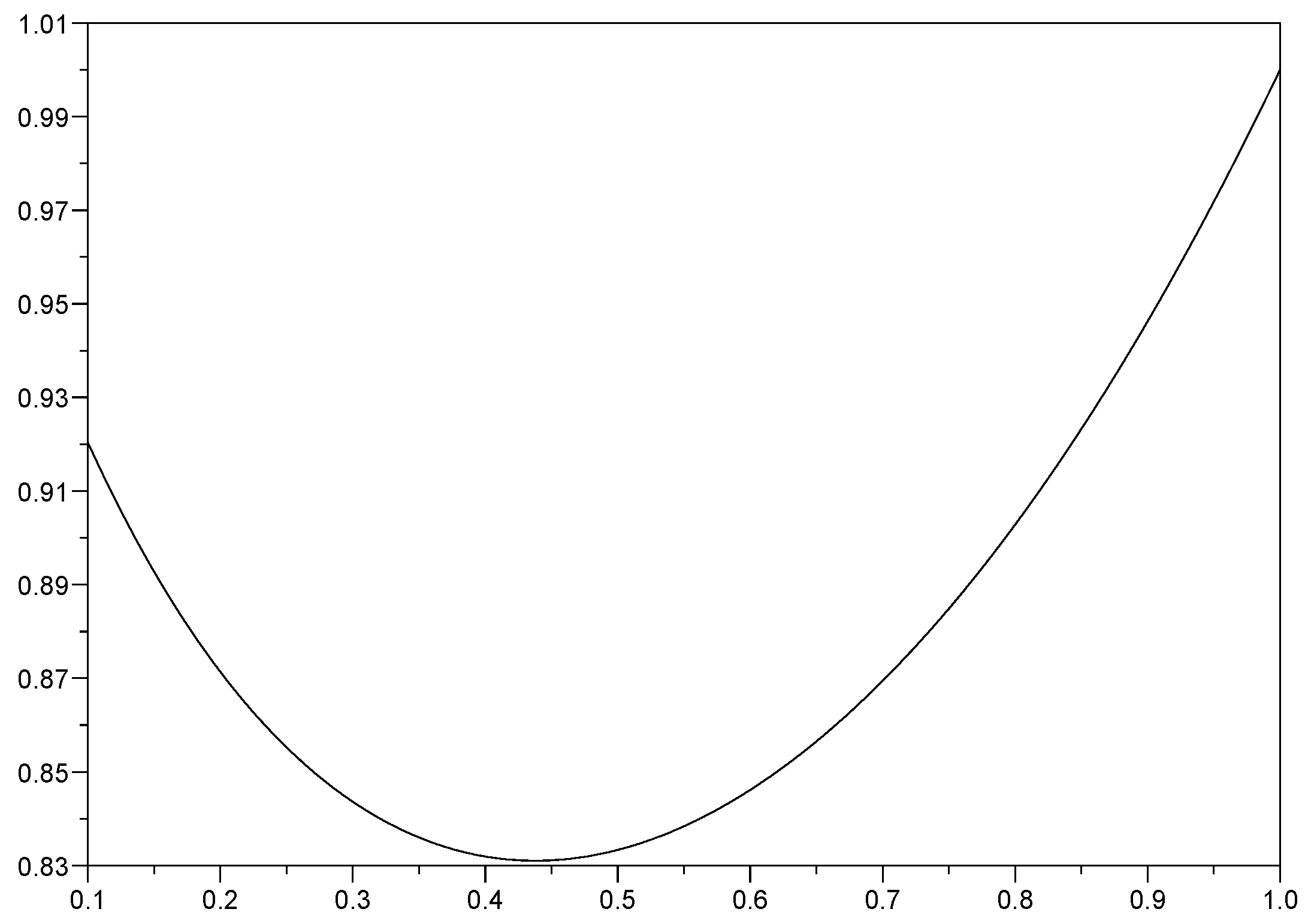
As we can see, for fixed u > 0 and H ( 0 , 1 ) , the covariance function c o v ( I H ( u ) , I H ( t ) ) of I H ( t ) = 0 t B H ( s ) d s is increasing as a function of t u , while, for fixed u and t , it first decreases as a function of H , then it increases, i.e., it admits a minimum.
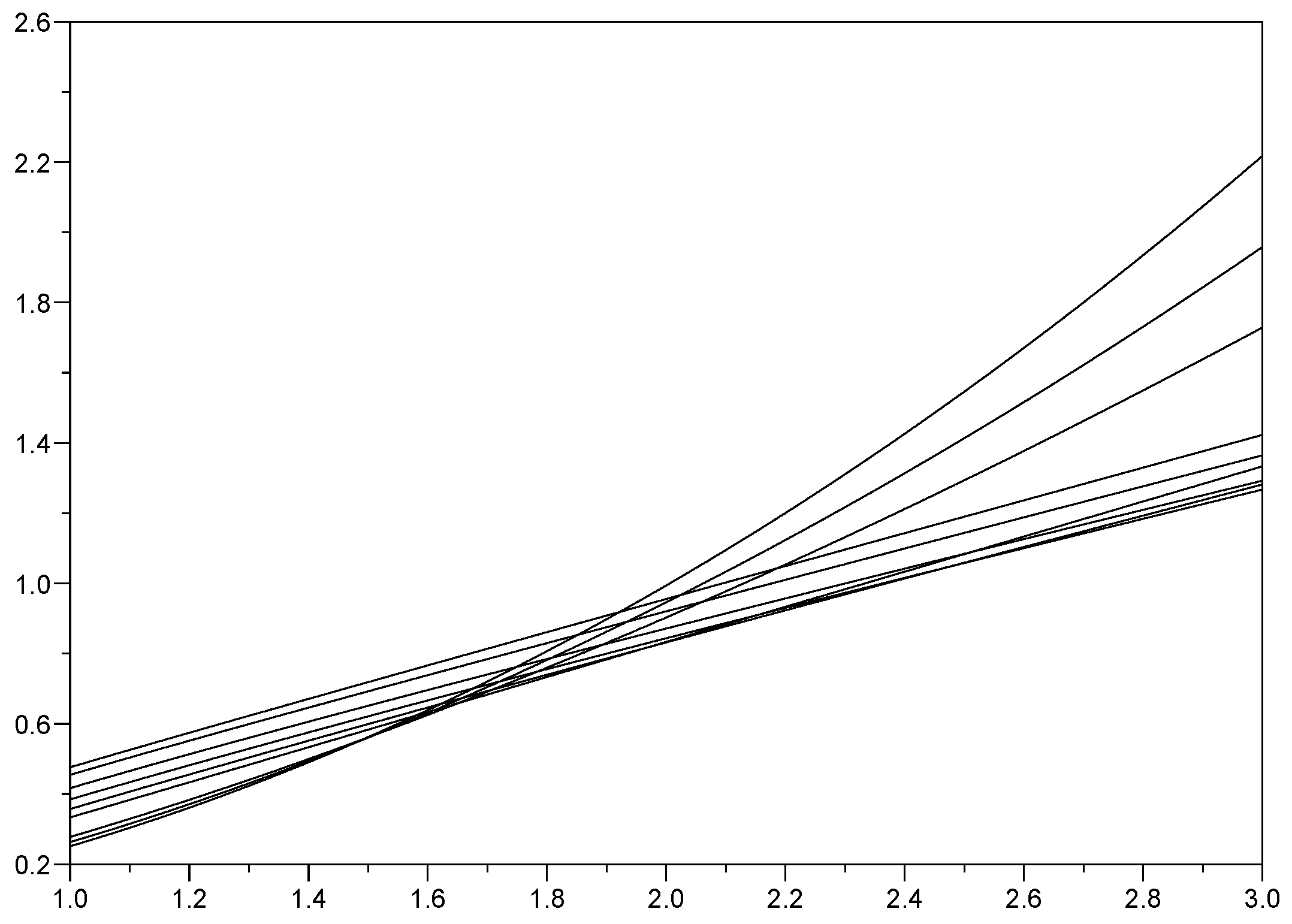
In Figure 2, we plot c o v ( I H ( u ) , I H ( t ) ) given by (20), as a function of t > u , for u = 1 fixed, and various values of H ( 0 , 1 ) . This figure presents some analogies with Figure 1 of [15], where the covariance function of the fractional Riemann–Liouville integral of BM of order α ( 0 , 1 ) is shown for various values of α .
In Figure 3, we plot the same covariance as a function of H ( 0 , 1 ) , for u = 1 and t = 2 .
Now, we consider the PFG process Y H ( t ) given by (8). The integral over time of Y H ( t ) is:
X H ( t ) = 0 t Y H ( s ) d s = 0 t ( m ( s ) + h 2 ( s ) B H ( r ( s ) ) ) d s ,
and it is again a Gaussian process (not necessarily self-similar); we call it an integrated pseudo-fractional Gaussian (IpFG) process. By proceeding as before for the integral of FBM I H ( t ) , we study the statistical parameters of IpFG process X H ( t ) . The mean of X H ( t ) is equal to 0 t m ( s ) d s , of course; for 0 u t , the covariance function is:
c H ( u , t ) : = c o v ( X H ( u ) , X H ( t ) ) = E 0 u h 2 ( s ) B H ( r ( s ) ) d s · 0 t h 2 ( v ) B H ( r ( v ) ) d v = 0 u d s 0 t d v h 2 ( s ) h 2 ( v ) E [ B H ( r ( s ) ) B H ( r ( v ) ) ] = 0 u d s 0 t d v h 2 ( s ) h 2 ( v ) · 1 2 r 2 H ( s ) + r 2 H ( v ) | r ( s ) r ( v ) | 2 H = 0 u d s 0 s d v h 2 ( s ) h 2 ( v ) · 1 2 r 2 H ( s ) + r 2 H ( v ) | r ( s ) r ( v ) | 2 H + 0 u d s s u d v h 2 ( s ) h 2 ( v ) · 1 2 r 2 H ( s ) + r 2 H ( v ) | r ( s ) r ( v ) | 2 H + 0 u d s u t d v h 2 ( s ) h 2 ( v ) · 1 2 r 2 H ( s ) + r 2 H ( v ) | r ( s ) r ( v ) | 2 H = 2 0 u d s 0 s d v h 2 ( s ) h 2 ( v ) · 1 2 r 2 H ( s ) + r 2 H ( v ) ( r ( s ) r ( v ) ) 2 H + 0 u d s u t d v h 2 ( s ) h 2 ( v ) · 1 2 r 2 H ( s ) + r 2 H ( v ) ( r ( v ) r ( s ) ) 2 H .
Taking u = t , one gets the variance:
v a r ( X H ( t ) ) = E 0 t h 2 ( s ) B H ( r ( s ) ) d s · 0 t h 2 ( u ) B H ( r ( u ) ) d u = 0 t d s 0 s d v h 2 ( s ) h 2 ( v ) r 2 H ( s ) + r 2 H ( v ) ( r ( s ) r ( v ) ) 2 H .
For H = 1 / 2 , one obtains covariance and variance of ordinary integral of a GM process (see [11]).
In conclusion, the covariance function and the variance of the IpFG process X H ( t ) , i.e., the integral of pFG process Y H ( t ) defined by (8), can be calculated substituting the function r ( t ) in (22) and (23), though formal calculations of the integrals involved are not easy, and sometimes it is more convenient to resort to numerical computation.
The knowledge of the covariance function of the IpFG process allows for studying the qualitative behavior of phenomena, especially in the framework of stochastic neuronal models, whose evolution is modeled by an IpFG process.

3. Comparisons with a Particular Fractional OU

We consider the process Z H ( t ) driven by Equation (15) with σ = 1 , already introduced by Kaarakka and Salminen ([24]), and called the fractional OU process of the first kind, with initial condition Z H ( 0 ) = z , where z is an assigned random variable. The solution process Z H ( t ) can be written as in (16), and using integration (pathwise) by parts in the Riemann–Stieltjes integral of (16), we can also write
Z H ( t ) = e μ t z + 0 t e μ s d B H ( s ) = e μ t z + B H ( t ) μ e μ t 0 t e μ s B H ( s ) d s .
The process Z H ( t ) is not a pFG process, but it involves the FBM and a particular weighted integral of FBM. It has mean:
E ( Z H ( t ) ) = e μ t E ( z ) .
Assuming E ( z ) = 0 , only for simplicity in writing, we show how its covariance can be written in terms of the covariance of FBM and IFBM; indeed, for s t , we have:
E ( Z H ( s ) Z H ( t ) ) = E e μ s z + B H ( s ) μ e μ s 0 s e μ w B H ( w ) d w e μ t z + B H ( t ) μ e μ t 0 t e μ v B H ( v ) d v = e μ s e μ t V a r ( z ) + E ( B H ( s ) B H ( t ) ) μ e μ t E B H ( s ) 0 t e μ v B H ( v ) d v μ e μ s E B H ( t ) 0 s e μ w B H ( w ) d w + μ 2 e μ s e μ t E 0 s e μ w B H ( w ) d w · 0 t e μ v B H ( v ) d v .
Finally, the covariance of Z H ( t ) as function of covariance E B H ( s ) B H ( t ) of FBM has the following expression:
E ( Z H ( s ) Z H ( t ) ) = e μ s e μ t V a r ( z ) + E B H ( s ) B H ( t ) μ e μ t 0 t e μ v E B H ( s ) B H ( v ) d v μ e μ s 0 s e μ w E B H ( t ) B H ( w ) d w + μ 2 e μ s e μ t 0 s e μ w 0 t e μ v E B H ( w ) B H ( v ) d w d v .
In addition, we can also make evident the relation of process Z H ( t ) with the IFBM I H ( t ) . Indeed, recalling that B H ( 0 ) = 0 , we can write
0 t e μ v B H ( v ) d v = e μ t I H ( t ) μ 0 t e μ v I H ( v ) d v
and, coming back to (25), we consider the term in the last parenthesis, and again we proceed by applying integration by parts in the following way:
E 0 s e μ w B H ( w ) d w · 0 t e μ v B H ( v ) d v = E e μ s I H ( s ) μ 0 s e μ w I H ( w ) d w e μ t I H ( t ) μ 0 t e μ v I H ( v ) d v = e μ ( s + t ) R H ( s , t ) μ e μ s 0 t e μ v R H ( s , v ) d v μ e μ t 0 s e μ w R H ( t , w ) d w + μ 2 0 s e μ w 0 t e μ v R H ( w , v ) d v d w ,
where we set R H ( s , t ) = C o v ( I H ( s ) I H ( t ) ) , i.e., (20). Finally, if we pose C H ( s , t ) = E ( B H ( s ) B H ( t ) ) , i.e., (1), taking into account (27), the following form of the covariance of Z H ( t ) holds:
E ( Z H ( s ) Z H ( t ) ) = e μ ( s + t ) V a r ( z ) + C H ( s , t ) μ e μ t 0 t e μ v C H ( s , v ) d v μ e μ s 0 s e μ w C H ( t , w ) d w + μ 2 R H ( s , t ) μ 3 e μ t 0 t e μ v R H ( s , v ) d v μ 3 e μ s 0 s e μ w R H ( t , w ) d w + μ 4 e μ ( s + t ) 0 s e μ w 0 t e μ v R H ( w , v ) d w d v .
Finally, re-ordering, we obtain the following representation:
E ( Z H ( s ) Z H ( t ) ) = e μ ( s + t ) V a r ( z ) + C H ( s , t ) + μ 2 R H ( s , t ) μ e μ t 0 t e μ v C H ( s , v ) + μ 2 R H ( s , v ) d v μ e μ s 0 s e μ w C H ( t , w ) + μ 2 R H ( t , w ) d w + μ 4 e μ ( s + t ) 0 s e μ w 0 t e μ v R H ( w , v ) d w d v .
Thus, the covariance of Z H ( t ) can be written in terms of the variance of the initial value z , the covariance, C H ( · , · ) , of FBM B H ( t ) , the covariance, R H ( · , · ) , of IFBM I H ( t ) , and some integrals involving functions of C H ( · , · ) and R H ( · , · ) .
As a final remark, we point out that the fractional OU process Z H ( t ) can also be represented by using FBM B H ( t ) , IFMB I H ( t ) , and the weighted integrated process of I H ( t ) , i.e.,
Z H ( t ) = e μ t z + B H ( t ) μ I H ( t ) + μ 2 e μ t 0 t e μ s I H ( s ) d s .
The last expression of Z H ( t ) can be used to design future neuronal models in which the stochastic evolution of the neuronal potential is described as a function of different dynamics modeled by the FBM and its integrals.

4. Conclusions and Final Remarks

In the present paper, we considered a new class of stochastic processes that we called a pseudo-fractional Gaussian process (pFG): they are obtained by the classical Doob representation of GM processes by replacing ordinary Brownian motion (BM) with fractional Brownian motion (FBM) with a Hurst index H ( 0 , 1 ) , We investigated the integral over time of such kind of pseudo-fractional Gaussian process; precisely, we studied the integral over time of the FBM and investigated its main statistical properties (mean and covariance). We defined the latter as the integrated FBM (IFBM).
Actually, GM processes and their time integrals have important applications in a variety of fields: in finance mathematics, in queueing theory, economy and other applied sciences, and mostly in computational neuroscience: especially in this context, there is the need to describe complex phenomena whose time evolution is affected by the history of their own behavior and by long range memory effects of different natures, which require to design more elaborate mathematical models relying on integrals over time of the involved stochastic processes. While in [15] the fractional RL integral of a GM process was studied, here we have dealt with its fractional counterpart concerning the noise: precisely, we have considered the ordinary Riemann integral, but involving pseudo-fractional GM processes instead of the classical GM ones. In other words, the fractional feature is shifted from the integral operator to the stochastic term that in the models is involved as the noise process. In fact, we have considered a pseudo-fractional Gauss process of the form Y H ( t ) = m ( t ) + h 2 ( t ) B H ( r ( t ) ) , where B H ( t ) is FBM with Hurst index H , and m ( t ) , h 2 ( t ) , r ( t ) are C 1 functions. Then, we have studied the main statistical properties of the integral over time of Y H ( t ) , namely the integrated pseudo-fractional Gauss (IpFG) process; we have found how varying the Hurst index H of the FBM affects its behavior, and we have put it into relation with the behavior of the fractional RL integral of the Gaussian Markov process Y 1 / 2 ( t ) , already studied in [15]. ( Y 1 / 2 ( t ) is obtained by replacing FBM with BM). Moreover, as an example of application, we have considered a particular fractional OU process Z H ( t ) , showing that its covariance function can be written in terms of the covariance functions of FBM, and IFBM; from this, it follows that the study of the IFBM provides useful information about the statistical properties of Z H ( t ) .
The wealth of behavior of the integral of the new kind of processes Y H ( t ) could be useful in the scope of neuronal stochastic models, which is a research field in which recently several fractional models have been proposed (see, e.g., [17,18] and references therein).

Author Contributions

Conceptualization, M.A. and E.P.; methodology, M.A. and E.P.; writing–original draft preparation, M.A. and E.P.; writing–review and editing, M.A. and E.P.

Funding

This research received no external funding.

Acknowledgments

We would like to express particular thanks to the anonymous referees for their constructive comments and suggestions leading to improvements of the paper. M.A. acknowledges the MIUR Excellence Department Project awarded to the Department of Mathematics, University of Rome Tor Vergata, CUP E83C18000100006; E.P. acknowledges the MIUR-PRIN 2017, project “Stochastic Models for Complex Systems”, No. 2017JFFHSH for a partial support to this work.

Conflicts of Interest

The authors declare no conflict of interest.

References

  1. Mura, A.; Taqqu, M.S.; Mainardi, F. Non-Markovian diffusion equations and processes: Analysis and simulations. Phys. A Stat. Mech. Its Appl. 2008, 387, 5033–5064. [Google Scholar] [CrossRef] [Green Version]
  2. Sokolov, I.M. Solutions of a class of non-Markovian Fokker–Planck equations. Phys. Rev. 2002, E66, 041101. [Google Scholar] [CrossRef] [PubMed]
  3. Baldovin, F.; Bovina, D.; Camana, F.; Stella, A.L. Modeling the Non-Markovian, Non-stationary Scaling Dynamics of Financial Markets. In Econophysics of Order-Driven Markets; Abergel, F., Chakrabarti, B.K., Chakraborti, A., Mitra, M., Eds.; New Economic Windows Springer: Milano, Italy, 2011. [Google Scholar]
  4. Barndorff-Nielsen, O.E.; Shephard, N. Integrated OU Processes and Non-Gaussian OU-based Stochastic Volatility Models. Scand. J. Stat. 2003, 30, 277–295. [Google Scholar] [CrossRef] [Green Version]
  5. Buonocore, A.; Caputo, L.; Pirozzi, E.; Carfora, M.F. Gauss-diffusion processes for modeling the dynamics of a couple of interacting neurons. Math. Biosci. Eng. 2014, 11, 189–201. [Google Scholar] [PubMed] [Green Version]
  6. Mura, I.; Prandi, D.; Priami, C.; Romanel, A. Exploiting non-Markovian Bio-Processes. Electron. Notes Theor. Comput. Sci. 2009, 253, 83–98. [Google Scholar] [CrossRef]
  7. Buonocore, A.; Caputo, L.; Pirozzi, E.; Carfora, M.F. A leaky integrate-and-fire model with adaptation for the generation of a spike train. Math. Biosci. Eng. 2016, 13, 483–493. [Google Scholar] [PubMed]
  8. D’Onofrio, G.; Pirozzi, E. Successive spike times pblackicted by a stochastic neuronal model with a variable input signal. Math. Biosci. Eng. 2016, 13, 495–507. [Google Scholar] [CrossRef] [PubMed]
  9. Pirozzi, E. Coloblack noise and a stochastic fractional model for correlated inputs and adaptation in neuronal firing. Biol. Cybern. 2018, 1–2, 25–39. [Google Scholar] [CrossRef] [PubMed]
  10. Abundo, M. On the representation of an integrated Gauss–Markov process. Sci. Math. Jpn. Online 2013, 77, 719–723. [Google Scholar]
  11. Abundo, M.; Pirozzi, E. Integrated stationary Ornstein–Uhlenbeck Process, and double integral processes. Phys. A Stat. Mech. Its Appl. 2018, 494, 265–275. [Google Scholar] [CrossRef]
  12. Abundo, M. On the first-passage time of an integrated Gauss–Markov process. Sci. Math. Jpn. Online 2015, 28, 1–14. [Google Scholar]
  13. Baleanu, D.; Diethelm, K.; Scalas, E.; Trujillo, J. Fractional Calculus: Models and Numerical Methods; World Scientific: Singapore, 2012; ISBN 978-981-4355-20-9. [Google Scholar] [CrossRef]
  14. Biagini, F.; Hu, Y.; Oksendal, B.; Zhang, T. Stochastic Calculus for Fractional Brownian Motion and Applications, Probability and Its Applications; Springer: Berlin/Heidelberg, Germany, 2010. [Google Scholar]
  15. Abundo, M.; Pirozzi, E. On the Fractional Riemann–Liouville Integral of Gauss–Markov processes and applications. arXiv 2019, arXiv:1905.08167. [Google Scholar]
  16. Mishura, Y. Stochastic Calculus for Fractional Brownian Motion and Related Processes; Lecture Notes in Mathematics; Springer: Berlin/Heidelberg, Germany, 1929. [Google Scholar]
  17. Abundo, M.; Ascione, G.; Carfora, M.F.; Pirozzi, E. A fractional PDE for first passage time of time-changed Brownian motion and its numerical solution. Appl. Numer. Math. 2019, in press. [Google Scholar] [CrossRef]
  18. Ascione, G.; Pirozzi, E. On a stochastic neuronal model integrating correlated inputs. Math. Biosci. Eng. 2019, 16, 5206–5225. [Google Scholar] [CrossRef] [PubMed]
  19. Kolmogorov, A.N. Wienersche Spiralen und einige andere interessante Kurven im Hilbertschen Raum. Acad. Sci. URSS (NS) 1940, 26, 115–118. [Google Scholar]
  20. Mandelbrot, B.B.; Van Ness, J.W. Fractional Brownian motion, fractional noise and applications. SIAM Rev. 1968, 10, 422–437. [Google Scholar] [CrossRef]
  21. Vardar, C. Results on the Supremum of Fractional Brownian Motion. arXiv 2012, arXiv:0910.5193v3. [Google Scholar]
  22. Ascione, G.; Mishura, Y.; Pirozzi, E. Fractional Ornstein–Uhlenbeck process with stochastic forcing, and its applications. 2019; submitted. [Google Scholar]
  23. Ascione, G.; Mishura, Y.; Pirozzi, E. Time-changed fractional Ornstein–Uhlenbeck process. arXiv 2019, arXiv:1907.04847. [Google Scholar]
  24. Kaarakka, T.; Salminen, P. On Fractional Ornstein–Uhlenbeck Processes. Commun. Stoch. Anal. 2011, 5, 121–133. [Google Scholar] [CrossRef]
  25. Cheridito, P.; Kowaguchi, H.; Maejima, M. Fractional Ornstein–Uhlenbeck processes. Electron. J. Probab. 2003, 8, 1–14. [Google Scholar] [CrossRef]
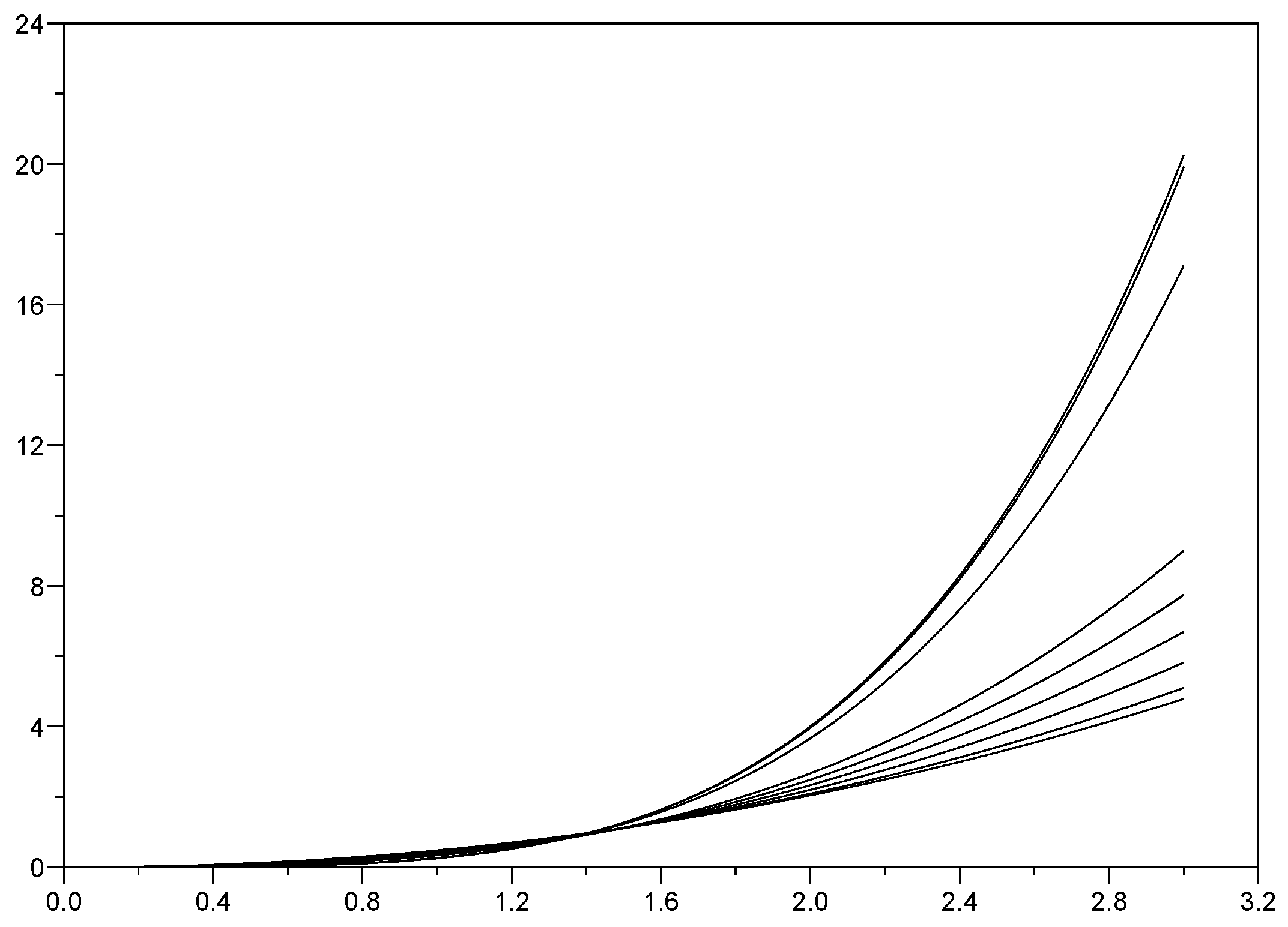
Figure 1. Plot of the variance of I H ( t ) = 0 t B H ( s ) d s , given by (19), as a function of t for various values of H ( 0 , 1 ) ; from bottom to top, with respect to the higher value at the right of t-axes, H = 0.05 , 0.1 , 0.2 , 0.3 , 0.4 , 0.5 , 0.8 , 0.9 , 0.99 .
Mathematics 07 00991 g001
Figure 2. Plot of the covariance function of I H ( t ) = 0 t B H ( s ) d s , given by (20), as a function of t > u , for u = 1 fixed, and various values of H ( 0 , 1 ) ; from bottom to top, with respect to the higher value at the right of t-axes, H = 0.05 , 0.1 , 0.2 , 0.3 , 0.4 , 0.5 , 0.8 , 0.9 , 0.99 .
Mathematics 07 00991 g002
Figure 3. Plot of the covariance function of I H ( t ) = 0 t B H ( s ) d s , given by (20), as a function of H ( 0 , 1 ) , for u = 1 and t = 2 .
Mathematics 07 00991 g003