A New Method for De-Noising of Well Test Pressure Data Base on Legendre Approximation

Abstract

In this paper, noise removing of the well test data is considered. We use the Legendre expansion to approximate well test data and a truncated strategy has been employed to reduce noise. The parameter of the truncation will be chosen by a discrepancy principle and a corresponding convergence result has been obtained. The theoretical analysis shows that a well numerical approximation can be obtained by the new method. Moreover, we can directly obtain the stable numerical derivatives of the pressure data in this method. Finally, we give some numerical tests to show the effectiveness of the method.

1. Introduction

Well test analysis is an important branch of reservoir engineering. In well test analysis, we can obtain some reservoir characteristics (reservoir permeability, wellbore storage coefficient, skin factor, drainage radius, etc.) by downhole pressure data which collected by permanent downhole gauges (PDG). Due to various reasons such as problems in gauges that occur by physical changes in reservoir, the original data from PDG usually contains large amounts of noise. Distorted data may cause high degree of uncertainty in well test interpretations and hence, PDG data have to be pre-processed before further analysis.

Noise removing is important in the process of analyzing well test data. The Butterworth digital filter method has been used by Osman and Stewart [1] to subtract noise in the data but it has poor performance in some cases such as have been shown by Kikani and He in Reference [2]. Instead, a wavelet analysis has been employed to remove noise. In Reference [3], Athichanagorn et al. proposed a seven-step procedure combining wavelet transform for the PDG data processing. Since then, numerous de-noising methods based on wavelet analysis have been present [4,5]. The main disadvantage of these methods is that their effect depend heavily on the selected wavelet types. In Reference [6], Nomura investigated a smoothing algorithm which utilized the derivative constraints to deal with PDG data. The data has been processed in log interval owing to the high degree of smoothness of the data in the log interval. He compared the constraint smoother and unconstrained regression splines and concluded that the former have better performance. But with the order of derivative constraints increases, the processing becomes more complex and the computational complexity increases greatly.

It is well known that using only pressure data for well test analysis may be insufficient and even may lead to misleading results. So the pressure derivative is useful in well test analysis. Up to now, all the existing methods need to redesign the calculation method of derivative on the basis of de-noising data. In recent years, numerical tools for inverse problems have been well developed [7,8] and we can obtain more stable approximation of derivatives. In this paper, we develop a method based on Legendre approximation for de-noising of well test pressure data which has been used to deal with the numerical differentiation problem [9]. The merit of the method is that we can directly obtain the approximation of derivatives. Because of its higher smoothness than the original interval, the data will be de-noised in logarithmic interval. We first obtain the Legendre approximation of the data and then the noise is eliminated by truncation. The parameter of the truncation will be chosen by a discrepancy principle. The method is implemented with Matlab and some numerical tests are utilized to verify the validity of the method.

2. The Theory of De-Nosing Based on Legendre Approximation

We first introduce some basic concepts and conclusions of Legendre approximation. Let $\Lambda =[-1,1]$ and denote by $L^2(\Lambda )$ and $H^r(\Lambda )$ the usual Lebesgue and Sobolev spaces and by $\parallel v\parallel$, ${\parallel v\parallel }_r$ their corresponding norms. The inner products of $L^2(\Lambda )$ and $H^m(\Lambda )$ are denoted by $\langle u,v\rangle$ and ${\langle u,v\rangle }_m$ respectively. Let N be any positive integer and ${\mathbb{P}}_N$ be the set of all algebraic polynomials of degree at most N in $\Lambda$. $P_N:L^2(\Lambda )\to {\left(P\right)}_N$ is the $L^2(\Lambda )-$orthogonal projection operator, that is,

$$\langle v-P_{N}v,\varphi \rangle =0,\forall \varphi \in {\mathbb{P}}_N.$$

(1)

Let $L_l\left(x\right)$ be the Legendre polynomial of degree l which can be defined by

$$L_l\left(x\right)=\frac{{(-1)}^l}{2^{l}l!}{\partial }_x^l{(1-x^2)}^l.$$

(2)

It well known that

$${\int }_{\Lambda }{L}_l\left(x\right)L_m\left(x\right)dx={\left(l+\frac{1}{2}\right)}^{-1}{\delta }_{l,m}.$$

(3)

So for any $f\in L^2(\Lambda )$, we may write

$$f\left(x\right)=\sum _{l=0}^{\infty }{\mathbf{f}}_l{L}_l\left(x\right)$$

(4)

with

$${\mathbf{f}}_l=\left(l+\frac{1}{2}\right){\int }_{\Lambda }f\left(x\right)L_l\left(x\right)dx.$$

(5)

Lemma 1.

[10] Let $r>0$, then for any $\varphi \in {\mathbb{P}}_N$,

$${\parallel \varphi \parallel }_r\le c{N}^{-2r}\parallel \varphi \parallel .$$

(6)

Lemma 2.

[10] For any $v\in H^r(\Lambda )$, $r>0$ and $\mu \le r$

$$\parallel v-P_N{v\parallel }_{\mu }\le c{N}^{\sigma (\mu ,r)}{\parallel v\parallel }_r,$$

(7)

where

$$\sigma (\mu ,r)=\left\{\begin{array}{cc}2\mu -r-\frac{1}{2},\hfill & \mu \ge 1,\hfill \\ \frac{3}{2}\mu -r,\hfill & 0\le \mu \le 1,\hfill \\ \mu -r,\hfill & \mu <0.\hfill \end{array}\right.$$

(8)

Let $x_0=-1,x_N=1$ and ${x_j}_{j=1}^{N-1}$ are the zeros of $L_N^{{}^{\prime }}\left(x\right)$ and

$${\omega }_j=\frac{2}{N(N+1){\left[L_N\left(x_j\right)\right]}^2},0\le j\le N.$$

(9)

${\Omega }_N$ is the set of all $x_j$. The discrete inner product in $C\left(\overline{\Omega }\right)$ and its associated norm can be defined by

$${\langle u,v\rangle }_{N,\omega }=\sum _{j=0}Nu\left(x_j\right)v\left(x_j\right){\omega }_j,{\parallel u\parallel }_{N,\omega }={\langle u,u\rangle }_{N,\omega }^{1/2}.$$

(10)

The Legendre interpolation $I_{N}v\left(x\right)\in {\mathcal{P}}_N$ of a function $v\in C\left(\overline{\Omega }\right)$ is defined by

$$I_{N}v\left(x_j\right)=v\left(x_j\right),\forall x_j\in {\Omega }_N.$$

(11)

Lemma 3.

[10] For any $v\in H^r(\Lambda )$, $0\le \mu \le 1$, $\mu <2r-1$,

$$\parallel v-I_N{v\parallel }_{\mu }\le c{N}^{\mu -r}{\parallel v\parallel }_r.$$

(12)

Now we present a noise removal algorithm base on Legendre expansion. Consider a signal $g\left(h_i\right),i=1,2,\dots ,n$ which is polluted by noise $e\left(h_i\right)$. That is to say, we only obtain its perturbed data:

$$g^{\delta }\left(h_i\right)=g\left(h_i\right)+e\left(h_i\right).$$

(13)

The process of de-noising involves obtaining approximate signal $\mathbf{g}\left(h_i\right)$ from noisy data $g^{\delta }\left(h_i\right)$. Our de-noising process is divided into the following steps:

• Transform the interval $[h_1,h_n]$ to the interval $[-1,1]$

  $${\widehat{h}}_i=\frac{2h_i-(h_1+h_n)}{h_n-h_1}$$

  (14)

  and an intermediate data ${\widehat{g}}^{\delta }$ is obtained by

  $${\widehat{g}}^{\delta }\left({\widehat{h}}_i\right)=g^{\delta }\left(h_i\right),i=1,2,\dots ,n.$$

  (15)
• Calculate the knots ${\Omega }_N$ and obtain the data ${\mathbf{g}}^{\delta }\left(x_j\right)$ by piecewise linear interpolation:

  $${\mathbf{g}}^{\delta }\left(x_0\right)={\widehat{g}}^{\delta }(-1),{\mathbf{g}}^{\delta }\left(x_N\right)={\widehat{g}}^{\delta }\left(1\right),{\mathbf{g}}^{\delta }\left(x_j\right)={\widehat{g}}^{\delta }\left({\widehat{h}}_{j0}\right)\frac{x_j-{\widehat{h}}_{j1}}{{\widehat{h}}_{j0}-{\widehat{h}}_{j1}}+{\widehat{g}}^{\delta }\left({\widehat{h}}_{j1}\right)\frac{x_j-{\widehat{h}}_{j0}}{{\widehat{h}}_{j1}-{\widehat{h}}_{j0}},$$

  (16)

  where ${\widehat{h}}_{j0}$ and ${\widehat{h}}_{j1}$ are the two nearest points of $x_j$ in ${\widehat{h}}_i,i=1,2,\dots ,n$.
• Obtain the Legendre interpolation function ${\widehat{\mathbf{g}}}_{\delta }$ by

  $${\widehat{\mathbf{g}}}_{\delta }=I_N{\mathbf{g}}^{\delta }.$$

  (17)
• Given the control parameter $\delta$(which can usually be estimated by the error distribution), the approximate signal ${\mathbf{g}}_{\delta }$ obtain by

  $${\mathbf{g}}_{\delta }=\left(P_m{I}_N{\mathbf{g}}^{\delta }\right),$$

  (18)

  where the parameter $m=m(\delta ,I_N{\mathbf{g}}^{\delta })$ is determined by the following discrepancy principle

  $$\parallel (I-P_m)I_N{\mathbf{g}}^{\delta }{)\parallel }_N\le \tau \delta \le \parallel (I-P_{m-1})I_N{\mathbf{g}}^{\delta }{)\parallel }_N$$

  (19)

  with $\tau >1$.

Now, we derive convergence result for above Legendre approximation.

Theorem 4.

Suppose that $g\in H^r(\Lambda )$ and the data ${\mathbf{g}}^{\delta }$ satisfy

$$\parallel {\mathbf{g}}^{\delta }{-g\parallel }_N\le \delta ,{\parallel {\mathbf{g}}^{\delta }\parallel }_N>\tau \delta$$

(20)

and $\mathbf{g}$ is defined by (18) and (19), then we have

$$\parallel D^k({\mathbf{g}}_{\delta }-g)\parallel =O({\delta }^{\frac{r-2k}{r}}+N^{2k-r}).$$

(21)

Proof. 

In terms of (19), (20) and the triangle inequality

$$\begin{array}{ccc}\parallel I_{N}g-P_{m-1}{I}_{N}g\parallel \hfill & =\hfill & \parallel (I-P_{m-1})I_N{g}^{\delta }-(I-P_{m-1})(I_N{\mathbf{g}}^{\delta }-I_{N}g)\parallel \hfill \\ \hfill & \ge \hfill & \parallel (I-P_{m-1})I_N{\mathbf{g}}^{\delta }\parallel -\parallel (I-P_{m-1})(I_N{\mathbf{g}}^{\delta }-I_{N}g)\parallel \hfill \\ \hfill & \ge \hfill & (\tau -1)\delta .\hfill \end{array}$$

(22)

On the other hand, from Lemma 2, 3 and note that $m\le N$

$$\begin{array}{ccc}\parallel I_{N}g-P_{m-1}{I}_{N}g\parallel \hfill & =\hfill & \parallel I_{N}g-g+g-P_{m-1}g+P_{m-1}g-P_{m-1}{I}_{N}g\parallel \hfill \\ \hfill & =\hfill & \parallel (I-P_{m-1})(I_{N}g-g)+(I-P_{m-1})g\parallel \hfill \\ \hfill & \le \hfill & \parallel (I-I_N)g\parallel +\parallel (I-P_{m-1})g\parallel \hfill \\ \hfill & \le \hfill & c{N}^{-r}{\parallel g\parallel }_r+c{(m-1)}^{-r}{\parallel g\parallel }_r\hfill \\ \hfill & \le \hfill & 2c{(m-1)}^{-r}{\parallel g\parallel }_r.\hfill \end{array}$$

(23)

Combining (22) with (23), we have

$$m\le {\left(\frac{{2c\parallel g\parallel }_r}{\tau -1}\right)}^{\frac{1}{r}}{\delta }^{-\frac{1}{r}}+1.$$

(24)

Moreover, by using the triangle inequality, Lemma 1, 2 and 3

$$\begin{array}{ccc}\parallel {\mathbf{g}}_{\delta }{-g\parallel }_{\frac{r}{2}}\hfill & =\hfill & \parallel P_m{I}_N{\mathbf{g}}^{\delta }-P_m{I}_{N}g+P_m{I}_{N}g-I_{N}g+I_N{g-g\parallel }_{\frac{r}{2}}\hfill \\ \hfill & \le \hfill & \parallel P_m(I_N{\mathbf{g}}^{\delta }-I_{N}g){\parallel }_{\frac{r}{2}}+\parallel (I-P_m)I_N{g\parallel }_{\frac{r}{2}}+{\parallel I_{N}g-g\parallel }_{\frac{r}{2}}\hfill \\ \hfill & \le \hfill & m^r\delta +m^{-\frac{1}{2}}\parallel I_N{g\parallel }_r+c{N}^{-\frac{r}{2}}{\parallel g\parallel }_r\hfill \end{array}$$

(25)

And from Lemma 3,

$$\parallel I_N{g\parallel }_r\le \parallel g-I_N{g\parallel }_r+{\parallel g\parallel }_r\le (c+1){\parallel g\parallel }_r.$$

(26)

By (24), (25) and (26), there exist a constant M such that

$$\parallel {\mathbf{g}}_{\delta }{-g\parallel }_{\frac{r}{2}}\le M.$$

(27)

Moreover,

$$\parallel {\mathbf{g}}_{\delta }-g\parallel \le \parallel P_m{I}_N{\mathbf{g}}^{\delta }-I_N{\mathbf{g}}^{\delta }\parallel +\parallel I_N{\mathbf{g}}^{\delta }-I_{N}g\parallel +\parallel I_{N}g-g\parallel \le (\tau +1)\delta +c{N}^{-r}{\parallel g\parallel }_r.$$

(28)

By interpolation inequality in [10]

$$\parallel D^k({\mathbf{g}}_{\delta }-g)\parallel \le \parallel {\mathbf{g}}_{\delta }{-g\parallel }_k\le \parallel {\mathbf{g}}_{\delta }{-g\parallel }_{\frac{r}{2}}^{\frac{2k}{r}}{\parallel {\mathbf{g}}_{\delta }-g\parallel }^{\frac{r-2k}{r}}.$$

(29)

From (27), (28) and (29), the approximation order (21) is proved. □

3. Numerical Tests

3.1. Preliminary Check for Approximation Capability of Legendre Expansion with Various Numbers of Knots

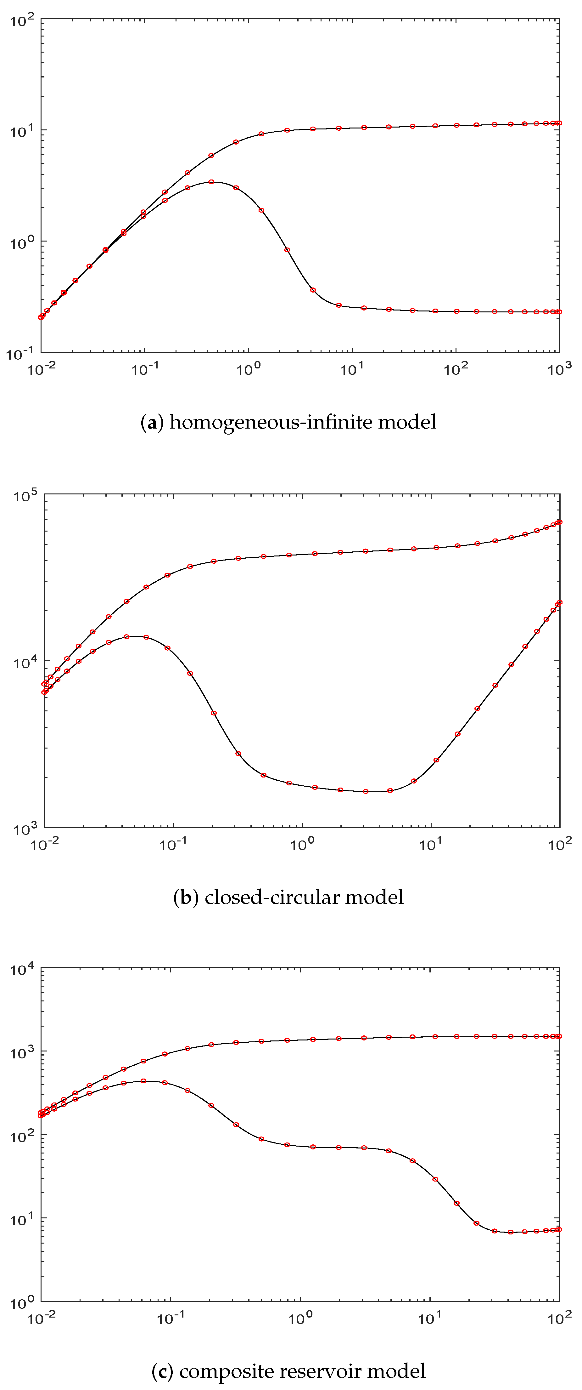
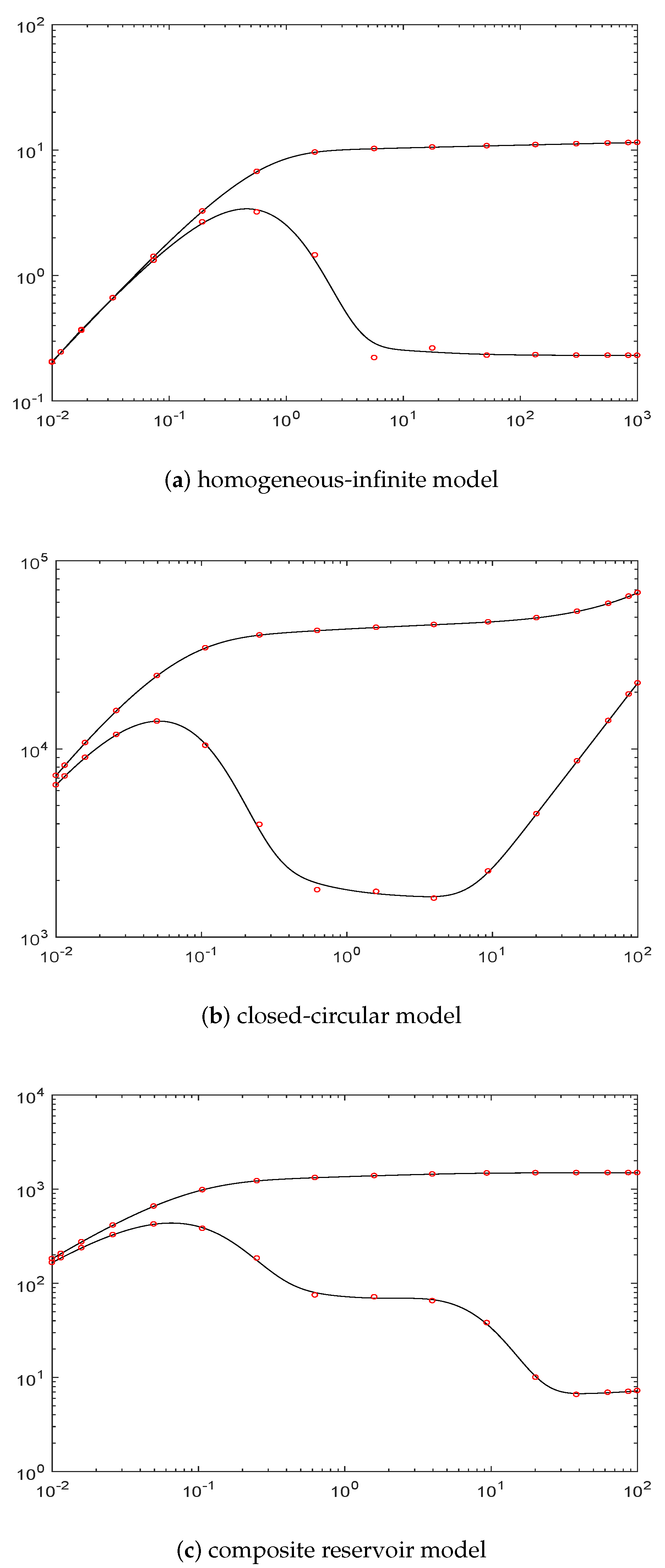
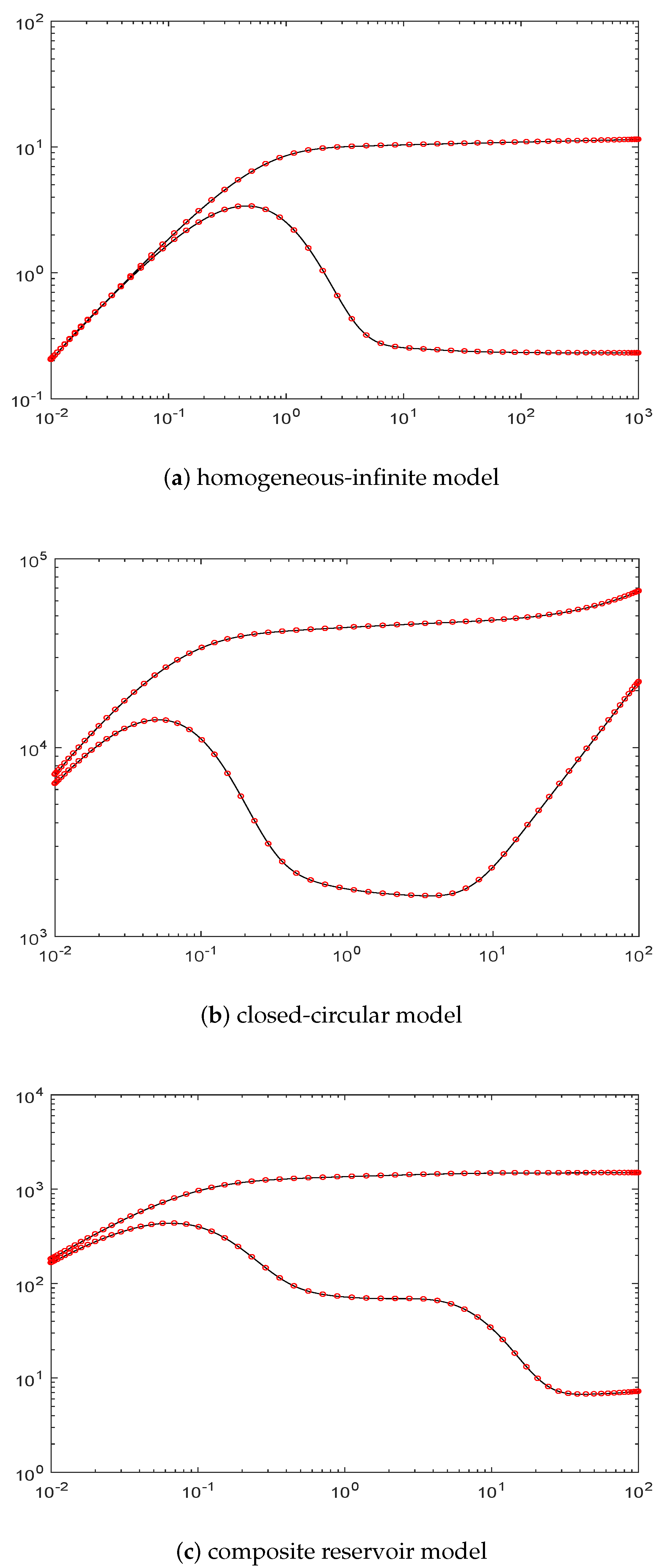
In general, more knots tends to give more approximation quality but this is unfavorable due to the increased model complexities and also for the computational burden. So we first check the effect of knots N number to approximate accurate data for three reservoir models [11]; the homogeneous-infinite model, the closed-circular model and the composite reservoir model. Their dimensionless well bore pressures in the Laplace space are respectively

• Homogeneous-infinite model:

  $${\overline{p}}_D=\frac{K_0\left(\sqrt{z}\right)+S\sqrt{z}{K}_1\left(\sqrt{z}\right)}{z\left[\sqrt{z}{K}_1\left(\sqrt{z}\right)+C_{D}z\left(K_0\left(\sqrt{z}\right)+S\sqrt{z}{K}_1\left(\sqrt{z}\right)\right)\right]},$$

  (30)

  where ${\overline{p}}_D$ is the dimensionless well-bore pressure in the Laplace space, z is the Laplace-transform parameter, $K_{\alpha }$ is the modified Bessel function of second-kind, of order $\alpha$, S is the skin factor, $C_D$ is the dimensionless wellbore storage coefficient.
• Closed-circular model:

  $${\overline{p}}_D=A{I}_0\left(r_D\sqrt{z}\right)+B{K}_0\left(r_D\sqrt{z}\right)-s\sqrt{z}(A{I}_1\left(\sqrt{z}\right)-B{K}_1\left(\sqrt{z}\right))$$

  (31)

  with

  $$A=\frac{K_1\left(r_{D_e}\sqrt{z}\right)}{z\left\{C_{D}z\left[K_1\left(r_{D_e}\sqrt{z}\right)I_0\left(r_D\sqrt{z}\right)+K_0\left(r_D\sqrt{z}\right)I_1\left(r_{D_e}\sqrt{z}\right)+s\sqrt{z}(-K_1\left(r_{D_e}\sqrt{z}\right)I_1\left(\sqrt{z}\right)+K_1\left(\sqrt{z}\right)I_1\left(r_{D_e}\sqrt{z}\right))\right]+\sqrt{z}(-K_1\left(r_{D_e}\sqrt{z}\right)I_1\left(\sqrt{z}\right)+K_1\left(\sqrt{z}\right)I_1\left(r_{D_e}\sqrt{z}\right))\right\}}$$

  (32)

  $$B=\frac{I_1\left(r_{D_e}\sqrt{z}\right)}{z\left\{C_{D}z\left[K_1\left(r_{D_e}\sqrt{z}\right)I_0\left(r_D\sqrt{z}\right)+K_0\left(r_D\sqrt{z}\right)I_1\left(r_{D_e}\sqrt{z}\right)+s\sqrt{z}(-K_1\left(r_{D_e}\sqrt{z}\right)I_1\left(\sqrt{z}\right)+K_1\left(\sqrt{z}\right)I_1\left(r_{D_e}\sqrt{z}\right))\right]+\sqrt{z}(-K_1\left(r_{D_e}\sqrt{z}\right)I_1\left(\sqrt{z}\right)+K_1\left(\sqrt{z}\right)I_1\left(r_{D_e}\sqrt{z}\right))\right\}}$$

  (33)

  where $r_{D_e}$ is the dimensionless outer radius and $I_{\alpha }$ is the modified Bessel function of the first-kind, of order $\alpha$.
• Composite reservoir model:

  $${\overline{p}}_D=A_1{I}_0\left(\sqrt{z}\right)+B_1{K}_0\left(\sqrt{z}\right)-S\left[A_1\sqrt{z}{I}_1\left(\sqrt{z}\right)-B_1\sqrt{z}{K}_1\left(\sqrt{z}\right)\right]$$

  (34)

  with

  $$A_1=\frac{dh-eg}{z\left[a\right(dh-eg)-b(ch-ef\left)\right]},$$

  (35)

  $$B_1=\frac{ef-ch}{z\left[a\right(dh-eg)-b(ch-ef\left)\right]},$$

  (36)

  and

  $$\begin{array}{ccc}a=C_{D}z{I}_0\left(\sqrt{z}\right)-(1+S{C}_{D}z)\sqrt{z}{I}_1\left(\sqrt{z}\right)\hfill & ,\hfill & b=C_{D}z{K}_0\left(\sqrt{z}\right)-(1+S{C}_{D}z)\sqrt{z}{K}_1\left(\sqrt{z}\right),\hfill \\ c=I_0\left(r_{\alpha }\sqrt{z}\right),d=K_0\left(r_{\alpha }\sqrt{z}\right)\hfill & ,\hfill & e=-K_0\left(r_{\alpha }\sqrt{\sigma z}\right),f=I_1\left(r_{\alpha }\sqrt{z}\right),\hfill \\ g=-K_1\left(r_{\alpha }\sqrt{z}\right),h=\lambda \sqrt{\sigma }{K}_1\left(r_{\alpha }\sqrt{\sigma z}\right).\hfill \end{array}$$

  (37)

  where $r_{\alpha }$ is the dimensionless radius inner zone, $\lambda$ is the Flow ratio and $\sigma$ is the storage capacity ratio.

The inversion form ${\overline{p}}_D$ to $p_D$ (the exact function g) is done using the Gaver-Stehfest algorithm [12]. We give the accurate data $g\left(h_i\right)$ at $h_i={10}^{-2+\frac{4i}{n}},i=0,1,2,\dots ,n$, $n=800$. Further, an interpolation function is given, similar to the one given in Formulas (15)–(18) ($\delta =0$). Figure 1, Figure 2 and Figure 3 show the fitting results of three models for $N=16,32,$ and 64. In the figures, the circles show the estimates at the knot locations. As shown here, more knots can give a better approximation quality and all the models are already fitted well to the true solution when $N=32$. So for the rest of examples, we always take $N=32$.

3.2. Tests for Validity of Method

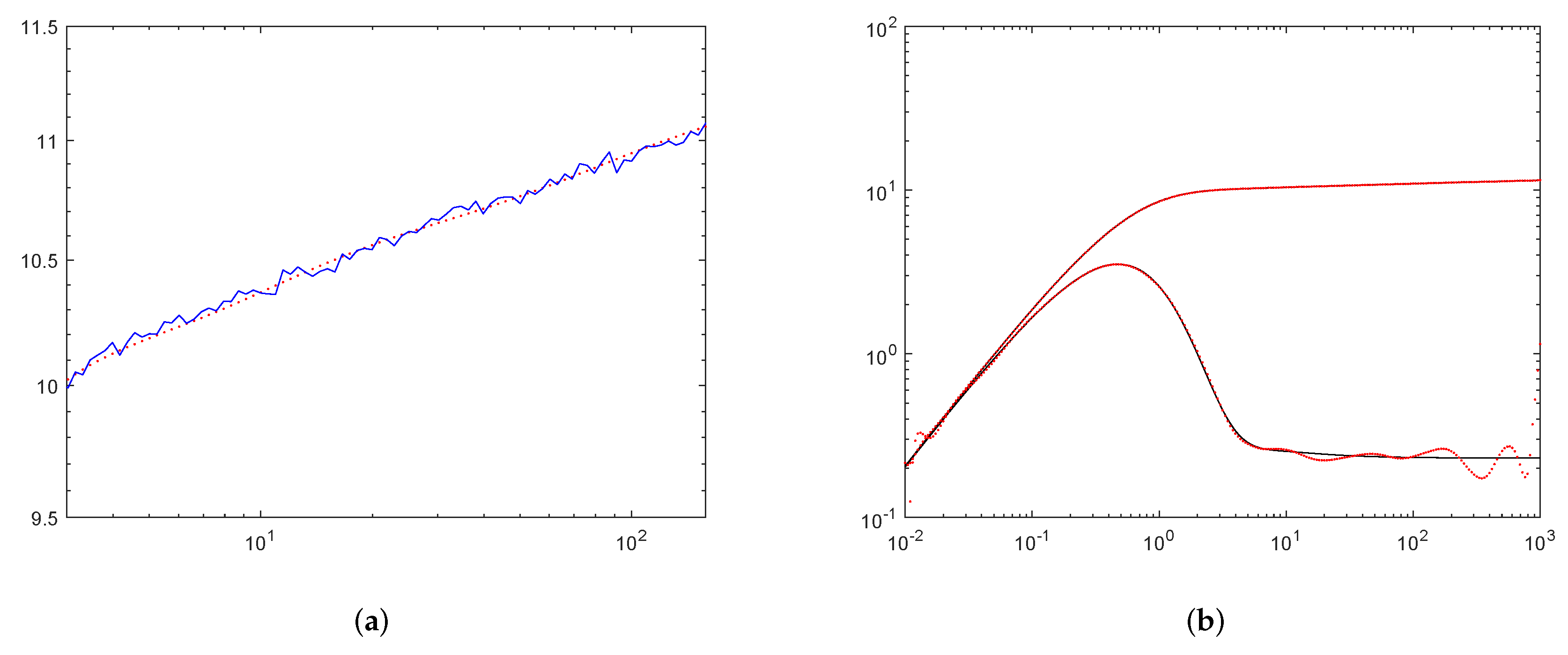
We added noise to the data as follows:

$$g^{\delta }\left(h_i\right)=g\left(h_i\right)+{ϵ}_i,i=0,1,\dots ,n,$$

(38)

where ${\left\{{ϵ}_i\right\}}_{j=0}^N$ are obtained by Matlab function $\mathrm{randn}(n+1,1)\times {\delta }_1$.

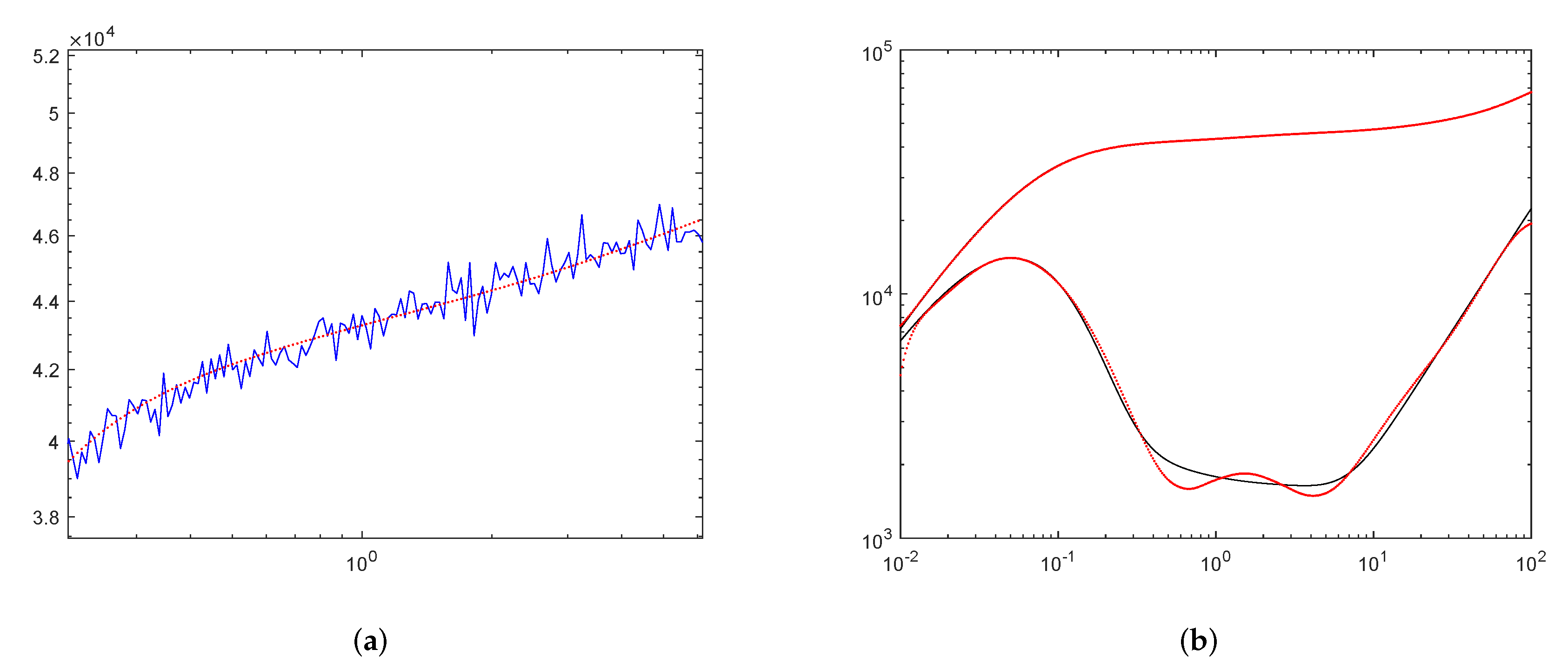
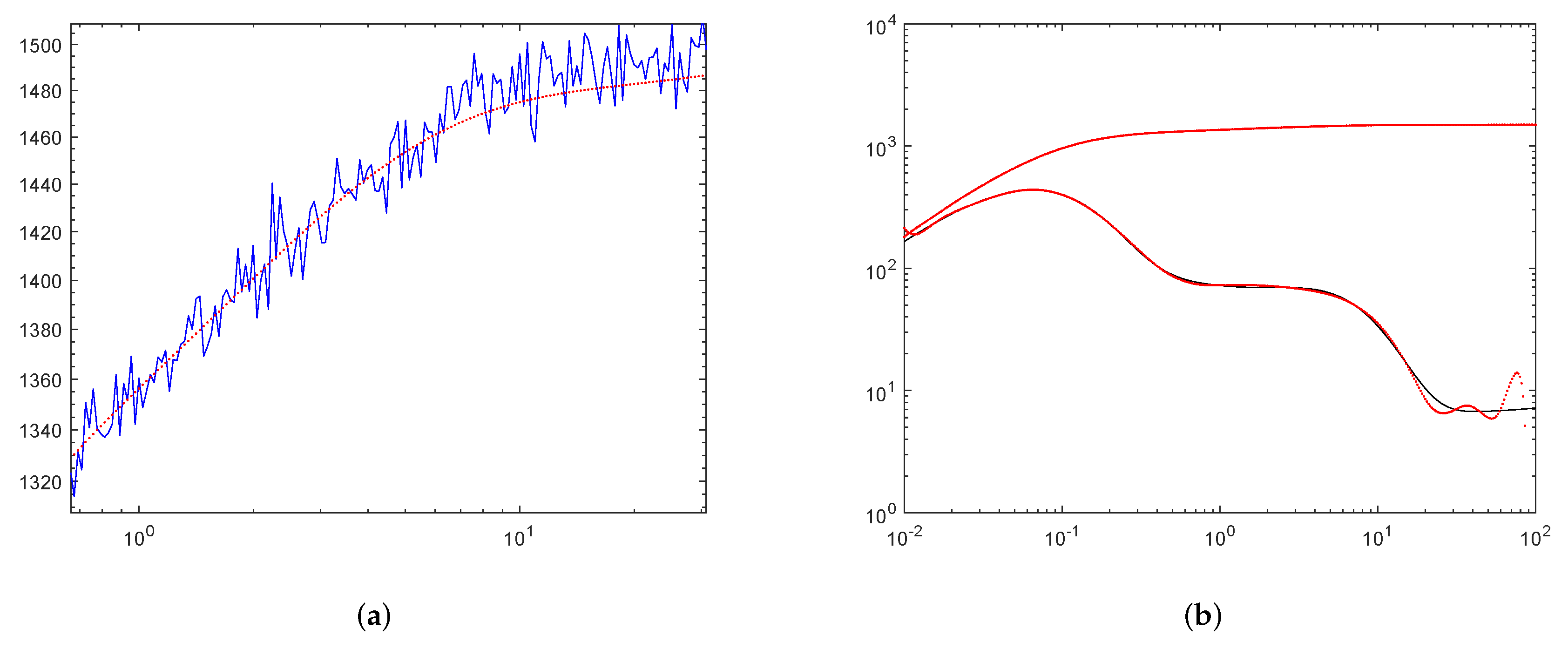
Figure 4, Figure 5 and Figure 6 show the fitting results of three models respectively. In each Figure, the first sub-figure gives a comparison between the noisy function and the de-noised one. The solid blue curves represents the noisy functions and the red dotted curves indicate the de-noised ones and we only took a partial of the curves to make the contrast more obvious. The second sub-figure shows that the comparisons of de-noised solution and its derivative with their corresponding accurate data. As can be seen, the performance of the method is satisfactory.

4. Conclusions

A new method to remove the noise of well test data based on the Legendre approximation is present in this paper. Benefit from the high accuracy of Legendre approximation, we can give a well approximation of well test data. The convergence result has been obtained and numerical tests have also verified the effectiveness of the method.

References

- Osman, M.S.; Stewart, G. Pressure data filtering and horizontalwell test analysis case study. In Proceedings of the Middle East Oil Show and Conference, Paper SPE 37802, Manama, Bahrain, 15–18 March 1997. [Google Scholar]
- Kikani, J.; He, M. Multi-resolution analysis of long-term pressure transient data using wavelet methods. In Proceedings of the SPE Annual Technical Conference and Exhibition, New Orleans, LA, USA, 27–30 September 1998. [Google Scholar]
- Athichanagorn, S.; Horne, R.N.; Kikani, J. Processing and interpretation of long-term data acquired from permanent pressure gauges. SPE Reserv. Eval. Eng. 2002, 5, 384–391. [Google Scholar] [CrossRef]
- Daubechies, I. The wavelet transform, time-frequency localization and signal analysis. IEEE Trans. Inf. Theory 1990, 36, 961–1005. [Google Scholar] [CrossRef]
- Olsen, S.; Nordtvedt, J. Automatic filtering and monitoring of real-time reservoir and production data. In Proceedings of the SPE Annual Technical Conference and Exhibition, Dallas, TX, USA, 9–12 October 2005. [Google Scholar]
- Nomura, M. Processing and Interpretation of Pressure Transient Data from Permanent Downhole Gauges. Ph.D. Thesis, Stanford University, Stanford, CA, USA, 2006. [Google Scholar]
- Hansen, C.P. Numerical tools for analysis and solution of Fredholm integral equations of the first kind. Inverse Probl. 1992, 8, 849–872. [Google Scholar] [CrossRef]
- Turco, E. Tools for the numerical solution of inverse problems in structural mechanics: Review and research perspectives. Eur. J. Environ. Civ. Eng. 2016, 21, 509–554. [Google Scholar] [CrossRef]
- Zhao, Z. A truncated legendre spectral method for solving numerical differentiation. Int. J. Comput. Math. 2010, 87, 3209–3217. [Google Scholar] [CrossRef]
- Guo, B.Y. Spectral Methods and their Applications; World Scientific: Singapore, 2010. [Google Scholar]
- Liu, Q. Modern Practical Method for Well Test Interpretation, 5th ed.; Petroleum Industry Press: Beijing, China, 2008. [Google Scholar]
- Gaver, G.P. Observing stochastic processes and approximate transform inversions. Oper. Res. 2003, 14, 444–459. [Google Scholar] [CrossRef]
© 2019 by the authors. Licensee MDPI, Basel, Switzerland. This article is an open access article distributed under the terms and conditions of the Creative Commons Attribution (CC BY) license (http://creativecommons.org/licenses/by/4.0/).