Fractional Order Unknown Inputs Fuzzy Observer for Takagi–Sugeno Systems with Unmeasurable Premise Variables

Abstract

This paper presents a new procedure for designing a fractional order unknown input observer (FOUIO) for nonlinear systems represented by a fractional-order Takagi–Sugeno (FOTS) model with unmeasurable premise variables (UPV). Most of the current research on fractional order systems considers models using measurable premise variables (MPV) and therefore cannot be utilized when premise variables are not measurable. The concept of the proposed is to model the FOTS with UPV into an uncertain FOTS model by presenting the estimated state in the model. First, the fractional-order extension of Lyapunov theory is used to investigate the convergence conditions of the FOUIO, and the linear matrix inequalities (LMIs) provide the stability condition. Secondly, performances of the proposed FOUIO are improved by the reduction of bounded external disturbances. Finally, an example is provided to clarify the proposed method. The obtained results show that a good convergence of the outputs and the state estimation errors were observed using the new proposed FOUIO.

1. Introduction

Recently, the interest in fractional derivatives and integral applications, as well as in theoretical and practical works, has grown immensely, see for example [1,2,3,4,5,6]. The main aspects, concept and several applications of fractional calculus are outlined, for example, in [7,8,9,10,11,12,13,14]. This is essentially due to the fact that various physical systems are well described by a fractional order state equation [15,16,17].

Growing applications have attracted interest in studying the state estimation of fractional differential equations in a linear case [18,19,20,21] and in a nonlinear case [22,23,24,25]. It is well known that the study of the problem of stabilization of the fractional order system is particularly important for the synthesis of the observer [26,27,28,29,30,31,32,33,34,35,36].

Takagi–Sugeno (TS) fuzzy models have also attracted attention in recent years. The main feature of this class of nonlinear models is to represent the local dynamics of each fuzzy implication (rule) by linear system models. It has been effectively employed in the implementation of nonlinear systems [37,38,39,40,41]. Takagi–Sugeno models have been broadly utilized to represent nonlinear integer-order systems. However, the fuzzy Takagi–Sugeno scheme remains very efficient for nonlinear fractional order systems (FOS) [42,43,44]. Therefore, the use of fractional-order Takagi–Sugeno (FOTS) models to represent nonlinear FOS will be introduced in this paper. Several approaches confirm that the validity functions of Takagi–Sugeno representation rely on measurable premise variables, whereas various applications, like diagnosis, consider that those variables rely on the input and state variables of the system that are usually immeasurable [45,46,47,48].

Takagi–Sugeno uses premise variables for computing weighting functions. Premise variables can be known (inputs or outputs of the system), or unknown variables taken as the state of the system to be estimated. State variables are usually unmeasurable, but they can be measured by the introduction of sensors, with an additional cost, but the right choice is to estimate the state variables in order to avoid the effects of sensor and shareholder faults that may have appeared on the inputs or outputs of the system considered. This justifies the research works on the state estimation of systems [48,49]. In order to use the state of the system as premise variables, then the states must be estimated, hence the need to synthesize an adequate observer able to estimate the state of the system despite the presence of unknown inputs and disturbances. Hence, it is motivating to deem the common state of unmeasurable variables such as system states. The problem appears especially in the structure of the state of the TS observer.

To implement a fuzzy observer for TS systems with unmeasurable premise variables (UPV), several methods have been evolved, comprising those which take account of analytical advances of an estimation error [50,51,52], and those which use the error description by a TS model with uncertainty or unorganized disruption [49]. The present work presents the Takagi–Sugeno unknown input fractional order observers design for FOTS models with UPV.

The main objective of the current paper is to found new stability and stabilization conditions using FOTS systems with UPV in the continuous case, to implement observers for nonlinear systems. The case where the weighting functions rely on premise variables depending on unmeasurable system states is considered. First, the representation of FOTS systems with UPV and their observers will be considered, which are given under the linear matrix inequalitie (LMI) formulation. Then, an analysis of the stability of the state estimation error studied by using the minimization of the $L_2$ norm of the transfer from bounded unknown exogenous disturbances to the state estimation error will be established. An application example is designed to demonstrate the performance of the suggested approach.

This paper is organized in the following way. The next section provides some background on the fractional calculus. The FOTS model is presented in Section 3. The main results of the paper, namely the synthesis of the fractional fuzzy observer based unmeasurable premise variables, are presented in Section 4. A new proposed method for unknown input estimation of the fractional order Takagi–Sugeno unknown input observer is given in Section 5. A numerical example is given in Section 6 to demonstrate the efficiency and validity of the proposed approach. Finally, the paper ends with concluding remarks and future perspectives in Section 7.

2. A Brief Introduction to Fractional Calculus

The fractional differo-integral operators are symbolized by ${}_a{D}_t^{\alpha }f\left(t\right)$, where a and t, are the bounds of the operation and $\alpha \in \mathbb{R}$ is a generalization of the standard integration and differentiation to an arbitrary order, which can be rational, irrational or even complex. The basic continuous differo-integral operator is given by the following:

$${}_a{D}_t^{\alpha }:=\left\{\begin{array}{ccc}\frac{d^{\alpha }}{d{t}^{\alpha }},& \mathrm{for}& \alpha >0,\\ 1,& \mathrm{for}& \alpha =0,\\ {\int }_a^t{\left(d\tau \right)}^{\alpha },& \mathrm{for}& \alpha <0.\end{array}\right.$$

(1)

In the literature, different definitions can be found concerning fractional order systems. The best most commonly used definitions of fractional order derivatives are:

The Riemann–Liouville (RL) definition [53]:

$${}_a{D}_t^{\alpha }f\left(t\right)=\frac{1}{\mathrm{\Gamma }(m-\alpha )}{\left(\frac{d}{dt}\right)}^m{\int }_a^t\frac{f\left(\tau \right)}{{(t-\tau )}^{1-(m-\alpha )}}d\tau .$$

(2)

The Grunwald–Letnikov (GL) definition [53]:

$${}_a{D}_t^{\alpha }f\left(t\right)=\underset{h\to 0}{lim}\frac{1}{h^{\alpha }}\sum _{k=0}^{(t-a)/h}{(-1)}^k\left(\begin{array}{c}\alpha \\ k\end{array}\right)f(t-kh).$$

(3)

The Caputo definition of the fractional differ-integral operator for the function $f\left(t\right)$ is adopted in this paper as the Caputo definition allows the initial values of classical integer-order derivatives with clear physical interpretation to be used as follows [51,53]:

$${}_a{D}_t^{\alpha }f\left(t\right)=\frac{1}{\mathrm{\Gamma }(m-\alpha )}{\int }_a^t\frac{f^m\left(\tau \right)}{{(t-\tau )}^{1-(m-\alpha )}}d\tau .$$

(4)

In these expressions $m-1<\alpha <m$, and $\mathrm{\Gamma }(.)$ is the well-known Eulers gamma function:

$$\mathrm{\Gamma }\left(x\right)={\int }_0^{\infty }{e}^{-t}{t}^{(x-1)}dt,x>0.$$

(5)

3. Fractional Order Takagi–Sugeno Model

Consider the following nonlinear system given by [54]:

$$\left\{\begin{array}{c}{}_a{D}_t^{\alpha }x\left(t\right)=f\left(x,u\right),\hfill \\ y\left(t\right)=g\left(x,u\right),\hfill \end{array}\right.$$

(6)

where $x\left(t\right)\in {\mathbb{R}}^n$ and $\alpha$ is the fractional order derivative. f and g are nonlinear functions.

Using the well-known transformation by nonlinear sector, the following TS fuzzy system is given [49]:

$$\left\{\begin{array}{c}{}_a{D}_t^{\alpha }x\left(t\right)={\displaystyle \sum _{i=0}^M}{h}_i\left(\xi \left(t\right)\right)\left[A_{i}x\left(t\right)+B_{i}u\left(t\right)\right],\hfill \\ y\left(t\right)={\displaystyle \sum _{i=0}^M}{h}_i\left(\xi \left(t\right)\right)\left[C_{i}x\left(t\right)+D_{i}u\left(t\right)\right],\hfill \end{array}\right.$$

(7)

where $u\left(t\right)\in {\mathbb{R}}^m$ is the input vector, $x\left(t\right)\in {\mathbb{R}}^n$ is the state vector, and $y\left(t\right)\in {\mathbb{R}}^p$ represents the output vector. $A_i\in {\mathbb{R}}^{n\times n}$, $B_i\in {\mathbb{R}}^{n\times n_u}$, $C_i\in {\mathbb{R}}^{n\times n_y}$ and $D_i\in {\mathbb{R}}^{n_y\times n_u}$ are known matrices. $h_i\left(\xi \left(t\right)\right)$ are the weighting functions relying on the premise variables $\xi \left(t\right)$ which can be measurable (input or output of the system) or unmeasurable variables (state of the system). It can also be an external signal. These functions confirm the following so-called convex sum property:

$$\left\{\begin{array}{c}{\displaystyle \sum _{i=0}^M}{h}_i\left(\xi \left(t\right)\right)=1,\hfill \\ 0\le h_i\left(\xi \left(t\right)\right)\le 1,\forall i\in \left\{1,2,\dots ,M\right\}.\hfill \end{array}\right.$$

(8)

In this paper, the target is to model a fractional order fuzzy TS observer with UPV. Thus, the work is dedicated to the problem of state estimation for nonlinear fractional order systems characterized by continuous time TS models, with unknown input $\overline{u}\left(t\right)$.

Under the hypothesis $C_1=C_2=\cdots =C$ and $D_i=0$, the FOTS model in the presence of unknown inputs and a measurable premise variable can be defined as follows:

$$\left\{\begin{array}{c}{}_a{D}_t^{\alpha }x\left(t\right)={\displaystyle \sum _{i=0}^M}{h}_i\left(x\left(t\right)\right)\left[A_{i}x\left(t\right)+B_{i}u\left(t\right)+E_i\overline{u}\left(t\right)\right],\hfill \\ y\left(t\right)=Cx\left(t\right)+E\overline{u}\left(t\right),\hfill \end{array}\right.$$

(9)

where $\overline{u}\left(t\right)\in {\mathbb{R}}^q$$(q<p)$ is the input vector, and $E_i\in {\mathbb{R}}^{n\times n_{\overline{u}}}$ and $E\in {\mathbb{R}}^{n_y\times n_{\overline{u}}}$ are known matrices. This can be rewritten as:

$$\left\{\begin{array}{c}{}_a{D}_t^{\alpha }x\left(t\right)={\displaystyle \sum _{i=0}^M}{h}_i\left(\widehat{x}\left(t\right)\right)\left[A_{i}x\left(t\right)+B_{i}u\left(t\right)+E_i\overline{u}\left(t\right)+\left(h_i\left(x\left(t\right)\right)-h_i\left(\widehat{x}\left(t\right)\right)\right)\left(A_{i}x\left(t\right)+B_{i}u\left(t\right)+E_i\overline{u}\left(t\right)\right)\right]\hfill \\ y\left(t\right)=Cx\left(t\right)+E\overline{u}\left(t\right).\hfill \end{array}\right.$$

(10)

After rewriting the model (9), we obtain:

$$\left\{\begin{array}{c}{}_a{D}_t^{\alpha }x\left(t\right)={\displaystyle \sum _{i=0}^M}{h}_i\left(\widehat{x}\left(t\right)\right)\left[A_{i}x\left(t\right)+B_{i}u\left(t\right)+E_i\overline{u}\left(t\right)+\omega \left(t\right)\right],\hfill \\ y\left(t\right)=Cx\left(t\right)+E\overline{u}\left(t\right).\hfill \end{array}\right.$$

(11)

This form corresponds to a perturbed FOTS model with measurable premise variables (estimated state of the system), where:

$$\omega \left(t\right)=\sum _{i=1}^M\left(h_i\left(x\left(t\right)-\widehat{x}\left(t\right)\right)\right)\left[A_{i}x\left(t\right)+B_{i}u\left(t\right)+E_i\overline{u}\left(t\right)\right].$$

(12)

This term is considered a global bounded and asymptotically vanishing perturbation.

4. Fractional Order Takagi–Sugeno Unknown Input Observer

The proposed fractional order Takagi–Sugeno fuzzy unknown input observer is given by the following equations:

$$\left\{\begin{array}{c}{}_a{D}_t^{\alpha }x\left(t\right)={\displaystyle \sum _{i=0}^M}{h}_i\left(\widehat{x}\left(t\right)\right)\left[N_{i}z\left(t\right)+G_{i}u\left(t\right)+L_{i}y\left(t\right)\right],\hfill \\ \widehat{x}\left(t\right)=z\left(t\right)+Hy\left(t\right).\hfill \end{array}\right.$$

(13)

The state and the output estimation can be defined as:

$$\begin{array}{c}\tilde{x}\left(t\right)=x\left(t\right)-\widehat{x}\left(t\right),\hfill \\ =x\left(t\right)-z\left(t\right)+HCx\left(t\right)+HE\overline{u}\left(t\right),\hfill \\ =Px\left(t\right)-z\left(t\right)+HE\overline{u}\left(t\right),\hfill \end{array}$$

(14)

where

$$P=I+HC.$$

(15)

Hence, the dynamics of the state estimation error is

$$\begin{array}{c}{}_{t_0}{D}_t^{\alpha }\widehat{x}\left(t\right)=P_{t_0}{D}_t^{\alpha }x\left(t\right){-}_{t_0}{D}_t^{\alpha }z\left(t\right)+H{E}_{t_0}{D}_t^{\alpha }\overline{u}\left(t\right)\hfill \\ ={\displaystyle \sum _{i=0}^M}{h}_i\left(\widehat{x}\left(t\right)\right)\left[P{A}_{i}x\left(t\right)+P{B}_{i}u\left(t\right)+P{E}_i\overline{u}\left(t\right)\right.\hfill \\ \left.+P\omega \left(t\right)-N_{i}z\left(t\right)-G_{i}u\left(t\right)-L_{i}y\left(t\right)\right]+H{E}_{t_0}{D}_t^{\alpha }\overline{u}\left(t\right),\hfill \end{array}$$

(16)

replacing $y\left(t\right)$ and $z\left(t\right)$ by their respective expressions given by (11) and (13), the state error is given as follows:

$$\begin{array}{c}{}_{t_0}{D}_t^{\alpha }\tilde{x}\left(t\right)={\displaystyle \sum _{i=0}^M}{h}_i\left(\widehat{x}\left(t\right)\right)\left[\left(P{A}_i-N_i-K_{i}C\right)x\left(t\right)+\left(P{B}_i-G_i\right)u\left(t\right)+\left(P{E}_i-K_{i}E\right)\overline{u}\left(t\right)+P\omega \left(t\right)\right.\hfill \\ \left.+N_{i}e\left(t\right)\right]+H{E}_{t_0}{D}_t^{\alpha }\overline{u}\left(t\right),\hfill \end{array}$$

(17)

with $K_i=N_{i}H+L_i$.

If the next conditions are satisfied:

$$HE=0,$$

(18)

$$N_i=P{A}_i-K_{i}C,$$

(19)

$$P{B}_i=G_i,$$

(20)

$$P{E}_i=K_{i}E$$

(21)

and

$$L_i=K_i-N_{i}H.$$

(22)

Then, the dynamics of the state estimation error become:

$${}_{t_0}{D}_t^{\alpha }\tilde{x}\left(t\right)=\sum _{i=1}^M{h}_i\left(\widehat{x}\left(t\right)\right)\left[N_i\tilde{x}\left(t\right)+P\omega \left(t\right)\right],$$

(23)

thus showing that the dynamics of the state estimation error is disturbed by $\omega \left(t\right)$.

To synthesize the matrices of the observer (13), two techniques are proposed.

4.1. First Approach

It is assumed that the term $\omega \left(t\right)$ defined in (12) satisfies the following Lipschitz condition:

$$\left|\omega \left(t\right)\right|\le \delta \left|\tilde{x}\left(t\right)\right|,$$

(24)

where $\delta$ is a positive constant.

Lemma 1

(see [55]). Let M and N be matrices of the appropriate sizes, then the following property holds:

$$M^{T}N+N^{T}M\le \eta M^{T}M+{\eta }^{-1}{N}^{T}N,\eta >0.$$

(25)

Theorem 1.

A fractional order unknown input observer (13) for system (11) exists if there exists a positive definite matrix X, matrices $M_i$, S, positive scalars η and δ satisfying the following conditions for all $i=1,\cdots ,M$:

$$\left[\begin{array}{cc}{\mathrm{\Theta }}_i& \left(X+SC\right)\\ {\left(X+SC\right)}^T& -\lambda I\end{array}\right]<0,$$

(26)

$$SE=0,$$

(27)

$$\left(X+SC\right)E_i=M_{i}E,$$

(28)

where

$${\mathrm{\Theta }}_i=A_i^T\left(X+C^{T}S\right)+\left(X+SC\right)A_i-C^T{M}_i^T-M_{i}C+\eta {\delta }^{2}I.$$

(29)

Then, the fractional order observer (13) is completely defined by:

$$H=X^{-1}S,$$

(30)

$$K_i=X^{-1}{M}_i,$$

(31)

$$N_i=\left(I+HC\right)A_i-K_{i}C,$$

(32)

$$L_i=K_i-N_{i}H,$$

(33)

and

$$G_i=\left(I+HC\right)B_i.$$

(34)

Proof of Theorem 1. 

In order to found the existence conditions of the fractional order observer in Theorem 1, Lemma 1 can be introduced:

Considering the following quadratic Lyapunov function:

$$V\left(t\right)=\tilde{x}{\left(t\right)}^{T}X\tilde{x}\left(t\right),X=X^T>0,$$

(35)

its derivative with regard to time is given by:

$${}_{t_0}{D}_t^{\alpha }V\left(t\right){\le }_{t_0}{D}_t^{\alpha }\tilde{x}{\left(t\right)}^{T}X\tilde{x}\left(t\right)\left(t\right)+\tilde{x}{\left(t\right)}^T{X}_{t_0}{D}_t^{\alpha }\tilde{x}\left(t\right).$$

(36)

By substituting (24), the dynamic of the quadratic Lyapunov function becomes:

$${}_{t_0}{D}_t^{\alpha }V\left(t\right)\le \sum _{i=1}^M{\mu }_i\left(\widehat{x}\left(t\right)\right)\left[\tilde{x}{\left(t\right)}^T\left(N_i^{T}X+X{N}_i\right)\tilde{x}\left(t\right)+\tilde{x}{\left(t\right)}^{T}XP\omega \left(t\right)+\omega {\left(t\right)}^T{P}^{T}X\tilde{x}\left(t\right)\right],$$

(37)

and when using Lemma 1 and (25), this allows for the following:

$$\begin{array}{c}{\tilde{x}}^{T}XP\omega +{\omega }^T{P}^{T}X\tilde{x}\le \eta {\omega }^T\omega +{\eta }^{-1}{\tilde{x}}^{T}XP{P}^{T}X\tilde{x}\hfill \\ \le \eta {\gamma }^2{\tilde{x}}^T\tilde{x}+{\eta }^{-1}{\tilde{x}}^{T}XP{P}^{T}X\tilde{x}.\hfill \end{array}$$

(38)

Substituting (38) in the fractional derivative of the Lyapunov function (36) yields:

$${}_{t_0}{D}_t^{\alpha }V=\sum _{i=1}^M{\mu }_i\left(\widehat{x}\right){\tilde{x}}^T\left(N_i^{T}X+X{N}_i+\eta {\gamma }^{2}I+{\eta }^{-1}XP{P}^{T}X\right)\tilde{x}.$$

(39)

Since the activation functions satisfy condition (8), the fractional derivative of the Lyapunov function is negative if:

$$N_i^{T}X+X{N}_i+\eta {\gamma }^{2}I+{\eta }^{-1}XP{P}^{T}X<0.$$

(40)

According to (19), Equation (40) becomes:

$${\left(P{A}_i-K_{i}C\right)}^{T}X+X\left(P{A}_i-K_{i}C\right)+\eta {\delta }^{2}I+{\eta }^{-1}XP{P}^{T}X<0.$$

(41)

It is noted unfortunately that the matrix inequality (41) gives a disadvantage since it is nonlinear with respect to the variables $K_i$, X and $\eta$ (more precisely bilinear). A numerical procedure of resolution by linearization is obtained in the following section.

In order to convert these conditions into an LMI formulation, the following change of variables is considered:

$$M_i=X{K}_i$$

(42)

and by using the Schur complement [16], the linear matrix inequality is obtained:

$$\left[\begin{array}{cc}{A}_i^T{P}^{T}X+XP{A_i-C}^T{M}_i^T+\eta {\delta }^{2}I& XP\\ P^{T}X& -\eta I\end{array}\right]<0.$$

(43)

To satisfy condition (18), the equality can be solved:

$$XHE=0.$$

(44)

Using the change of variable $S=XH$, linear matrix equality is obtained:

$$SE=0.$$

(45)

The conditions (21) must be satisfied simultaneously, and using the change of variable (42) gives:

$$\left(X+SC\right)E_i=M_{i}E.$$

(46)

Since $P=I+HC$, replacing P in (43), the matrix inequality of Theorem 1 can be obtained.

The conditions (26)–(28) of Theorem 1 are thus demonstrated. □

4.2. Second Approach

In the case where hypothesis (24) is not satisfied, meaning that the information on its bounded $\delta$ is not available, the method established in the previous section cannot be applied.

In this section, another method based on the use of the $L_2$ approach is proposed.

Theorem 2.

A fractional order unknown input observer (13) for system (11) exists if there exists a positive definite matrix X, matrices $M_i$, S and positive scalars $\overline{\delta }$ satisfying the following conditions for all $i=1,\cdots ,M$:

$$\left[\begin{array}{cc}{\mathrm{\Theta }}_i& X+SC\\ {\left(X+SC\right)}^T& -\overline{\gamma }I\end{array}\right]<0,$$

(47)

$$SE=0$$

(48)

and

$$\left(X+SC\right)E_i=M_{i}E,$$

(49)

where

$${\mathrm{\Theta }}_i=A_i^T\left(X+C^{T}S\right)+\left(X+SC\right)A_i-C^T{M}_i^T-M_{i}C+I.$$

(50)

Then, the fractional order UI observer (13) is completely defined by (30)–(34).

Proof of Theorem 2. 

To prove Theorem 2, the real bounded Lemma 1 [56] is used.

The dynamics of the fractional state estimation error are given by:

$${}_{t_0}{D}_t^{\alpha }\tilde{x}\left(t\right)=\sum _{i=1}^M{h}_i\left(\widehat{x}\left(t\right)\right)\left[N_i\tilde{x}\left(t\right)+P\omega \left(t\right)\right].$$

(51)

Consider the following Lyapunov quadratic function:

$$V\left(t\right)=\tilde{x}{\left(t\right)}^{T}X\tilde{x}\left(t\right),X=X^T>0.$$

(52)

Its derivative with regard to time is specified by:

$${}_{t_0}{D}_t^{\alpha }V\left(t\right){\le }_{t_0}{D}_t^{\alpha }\tilde{x}{\left(t\right)}^{T}X\tilde{x}\left(t\right)+\tilde{x}{\left(t\right)}^T{X}_{t_0}{D}_t^{\alpha }\tilde{x}\left(t\right).$$

(53)

By substituting (23), the dynamic of the quadratic Lyapunov function is obtained:

$${}_{t_0}{D}_t^{\alpha }V\left(t\right)\le \sum _{i=1}^M{\mu }_i\left(\widehat{x}\left(t\right)\right)\left[\tilde{x}{\left(t\right)}^T\left(N_i^{T}X+X{N}_i\right)\tilde{x}\left(t\right)+\tilde{x}{\left(t\right)}^{T}XP\omega \left(t\right)+\omega {\left(t\right)}^T{P}^{T}X\tilde{x}\left(t\right)\right].$$

(54)

In order to mitigate the impact of $\omega \left(t\right)$ on the state estimation error, the $L_2$ [52] will be used. It can guarantee:

$$\frac{{∥\tilde{x}\left(t\right)∥}_2}{{∥\omega \left(t\right)∥}_2}<\delta ,\delta >0.$$

(55)

The system of the state estimation error is stable and the gain $L_2$ noted $\delta$ of the transfer from $\omega \left(t\right)$ to $\tilde{x}\left(t\right)$ is bounded, if:

$${}_{t_0}{D}_t^{\alpha }V\left(\tilde{x}\left(t\right)\right)+\tilde{x}{\left(t\right)}^T\tilde{x}\left(t\right)-{\delta }^2\omega {\left(t\right)}^T\omega \left(t\right)<0.$$

(56)

By substituting ${}_{t_0}{D}_t^{\alpha }V\left(\tilde{x}\left(t\right)\right)$, the inequality (56) becomes:

$$\begin{array}{c}{\displaystyle \sum _{i=0}^M}{\mu }_i\left(\widehat{x}\left(t\right)\right)\left[\tilde{x}{\left(t\right)}^T\left(N_i^{T}X+X{N}_i\right)\tilde{x}\left(t\right)\right.+\tilde{x}{\left(t\right)}^{T}XP\omega \left(t\right)+\omega {\left(t\right)}^T{P}^{T}X\tilde{x}\left(t\right)\hfill \\ \left.+\tilde{x}{\left(t\right)}^T\tilde{x}\left(t\right)-{\delta }^2\omega {\left(t\right)}^T\omega \left(t\right)\right].\hfill \end{array}$$

(57)

The estimation error converges to zero and the gain $L_2$ of the transfer from $\omega \left(t\right)$ to $\tilde{x}\left(t\right)$ is bounded by $\delta$ if the following inequality is verified:

$$\sum _{i=1}^M{\mu }_i\left(\widehat{x}\left(t\right)\right)\left[\begin{array}{cc}{N}_i^{T}X+X{N}_i+I& XP\\ P^{T}X& -{\delta }^{2}I\end{array}\right]<0.$$

(58)

The convex sum property of the activation functions makes it possible to write the following sufficient condition:

$$\left[\begin{array}{cc}{N}_i^{T}X+X{N}_i+I& XP\\ P^{T}X& -{\delta }^{2}I\end{array}\right]<0.$$

(59)

Using the expression (19) of $N_i$ and the changes of variables $M_i=X{K}_i$ and $\overline{\delta }={\delta }^2$ (48) becomes:

$$\left[\begin{array}{cc}{\mathrm{\Theta }}_i& XP\\ P^{T}X& -\overline{\delta }I\end{array}\right]<0,\forall i=1,\dots ,M$$

(60)

where

$${\mathrm{\Theta }}_i=A_i^T{P}^{T}X+XP{A}_i-C^T{M}_i^T-M_{i}C+I.$$

To satisfy condition (18), the equality can be solved:

$$XHE=0.$$

(61)

Using the change of variable $S=XH$, the linear matrix equality is obtained:

$$SE=0.$$

(62)

The conditions (21) must be satisfied simultaneously, and by using the change of variable (42) gives:

$$\left(X+SC\right)E_i=M_{i}E.$$

(63)

Since $P=I+HC$, replacing P in (60), the matrix inequality of Theorem 2 is obtained.

The conditions (47)–(49) of Theorem 2 are thus demonstrated. □

5. Unknown Inputs Estimation

In system (11), the unknown input $\overline{u}\left(t\right)$ appears with the influence matrix:

$$\mathrm{\Phi }\left(t\right)=\left[\begin{array}{c}{\displaystyle \sum _{i=0}^M}{h_i\left(\widehat{x}\left(t\right)\right)E}_i\\ E\end{array}\right].$$

(64)

For the estimation of the unknown input, it is necessary that the rank of the matrix $\mathrm{\Phi }\left(t\right)$ is verified at each time t for the following condition:

$$\mathrm{rank}\left(\mathrm{\Phi }\left(t\right)\right)=q,$$

(65)

where q is the dimension of $\overline{u}\left(t\right)$. If this condition is satisfied, $\mathrm{\Phi }\left(t\right)$ is full-rank column and its pseudo-inverse left ${\mathrm{\Phi }}^{-1}\left(t\right)$ exists:

$${\mathrm{\Phi }}^{-}\left(t\right)={\left({\mathrm{\Phi }}^T\left(t\right)\mathrm{\Phi }\left(t\right)\right)}^{-1}{\mathrm{\Phi }}^T\left(t\right).$$

(66)

The unknown input can then be calculated according to the state estimated as follows:

$$\widehat{\overline{u}}\left(t\right)={\mathrm{\Phi }}^{-}\left[\begin{array}{c}{}_{t_0}{D}_t^{\alpha }\widehat{x}\left(t\right)-{\displaystyle \sum _{i=0}^M}{h}_i\left(\widehat{x}\left(t\right)\right)\left[A_i\widehat{x}\left(t\right)+B_{i}u\left(t\right)\right]\\ y\left(t\right)-C\widehat{x}\left(t\right)\end{array}\right],$$

(67)

under condition (65) the asymptotic convergence from $\widehat{x}\left(t\right)$ to $x\left(t\right)$ results in the asymptotic convergence of $\widehat{\overline{u}}\left(t\right)$ to $\overline{u}\left(t\right)$.

6. Example and Comparisons

To validate the advantages of the proposed fractional order unknown input observer, the system (68) represented by the FOTS model with UPV is considered with $\alpha =0.8$. The state estimation is carried out by means of two fuzzy unknown input observers, the first with integer order and the second one with fractional order. The unknown inputs considered may be noise, faults or modeling uncertainties.

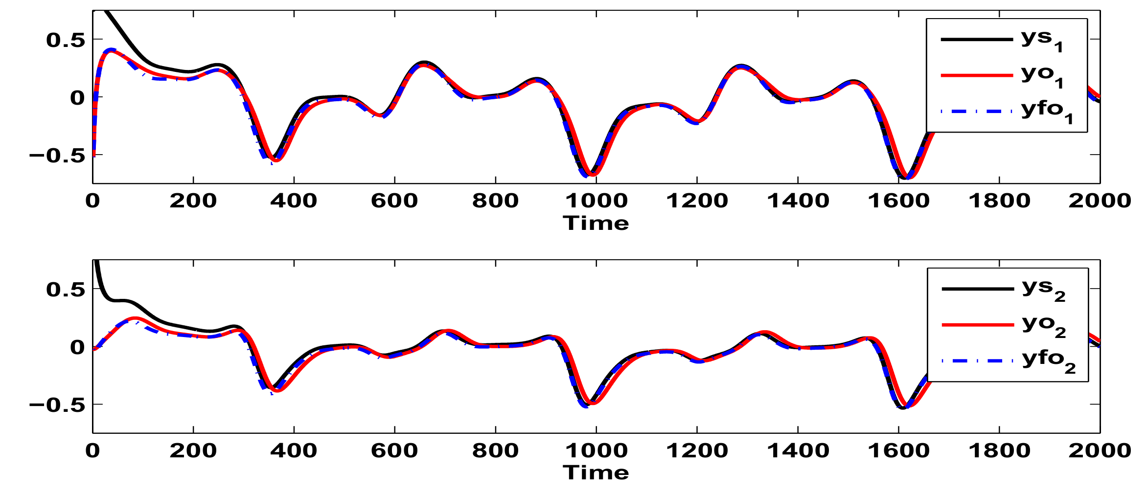
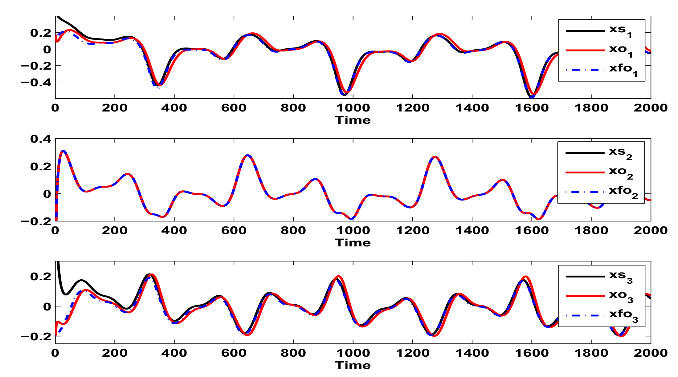
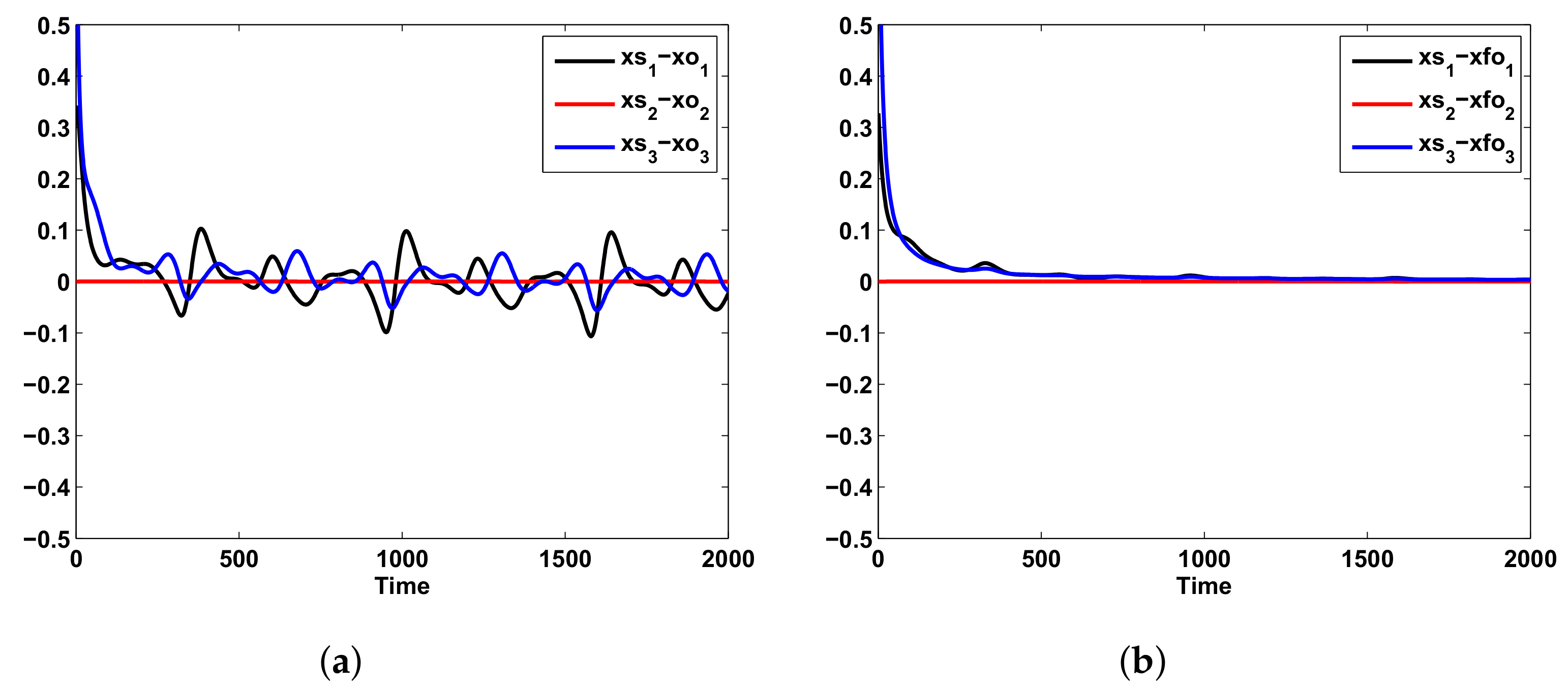
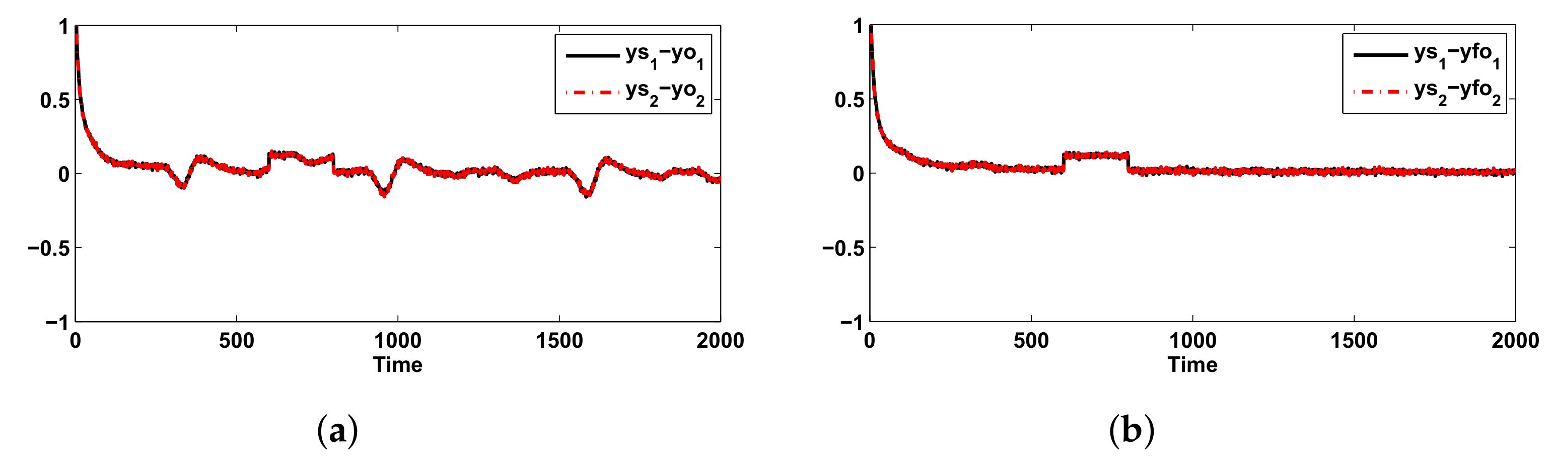
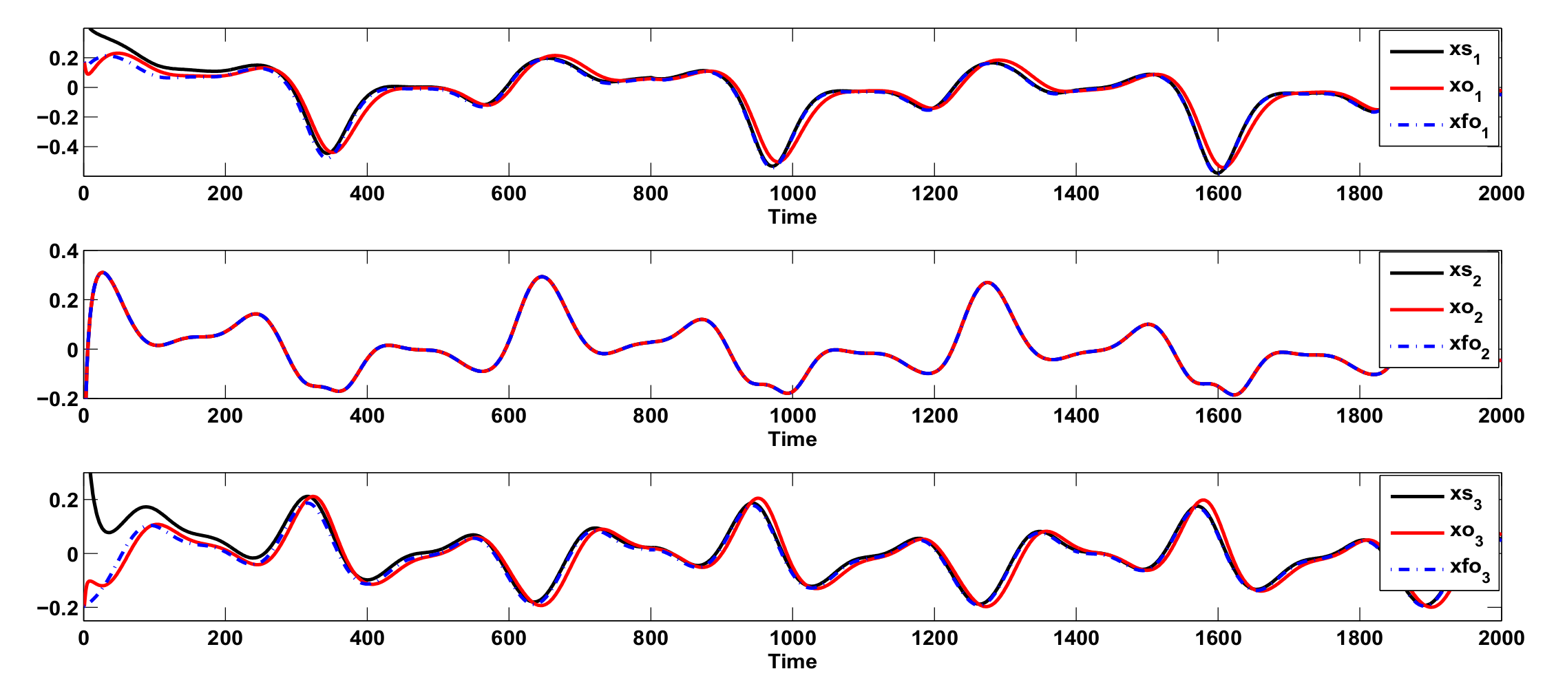
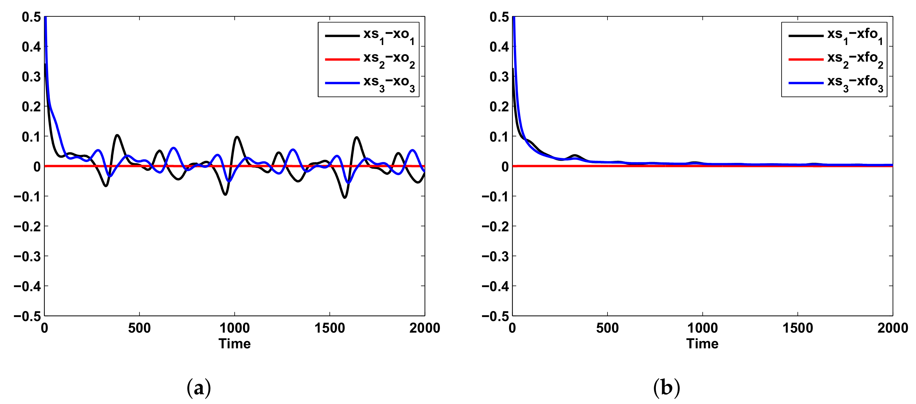
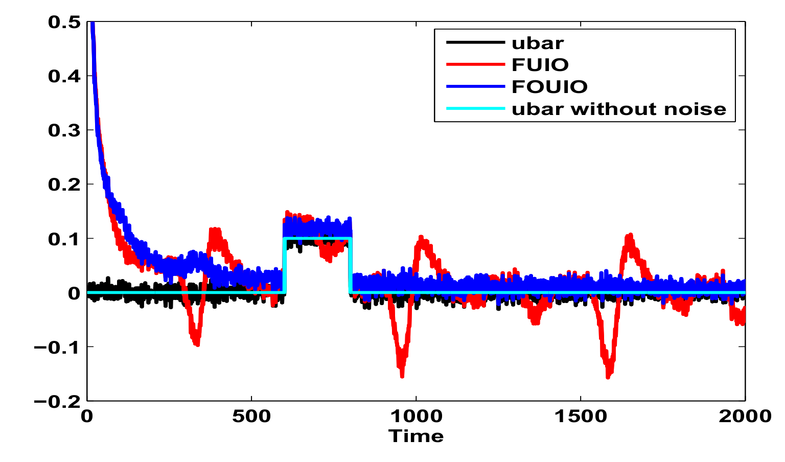
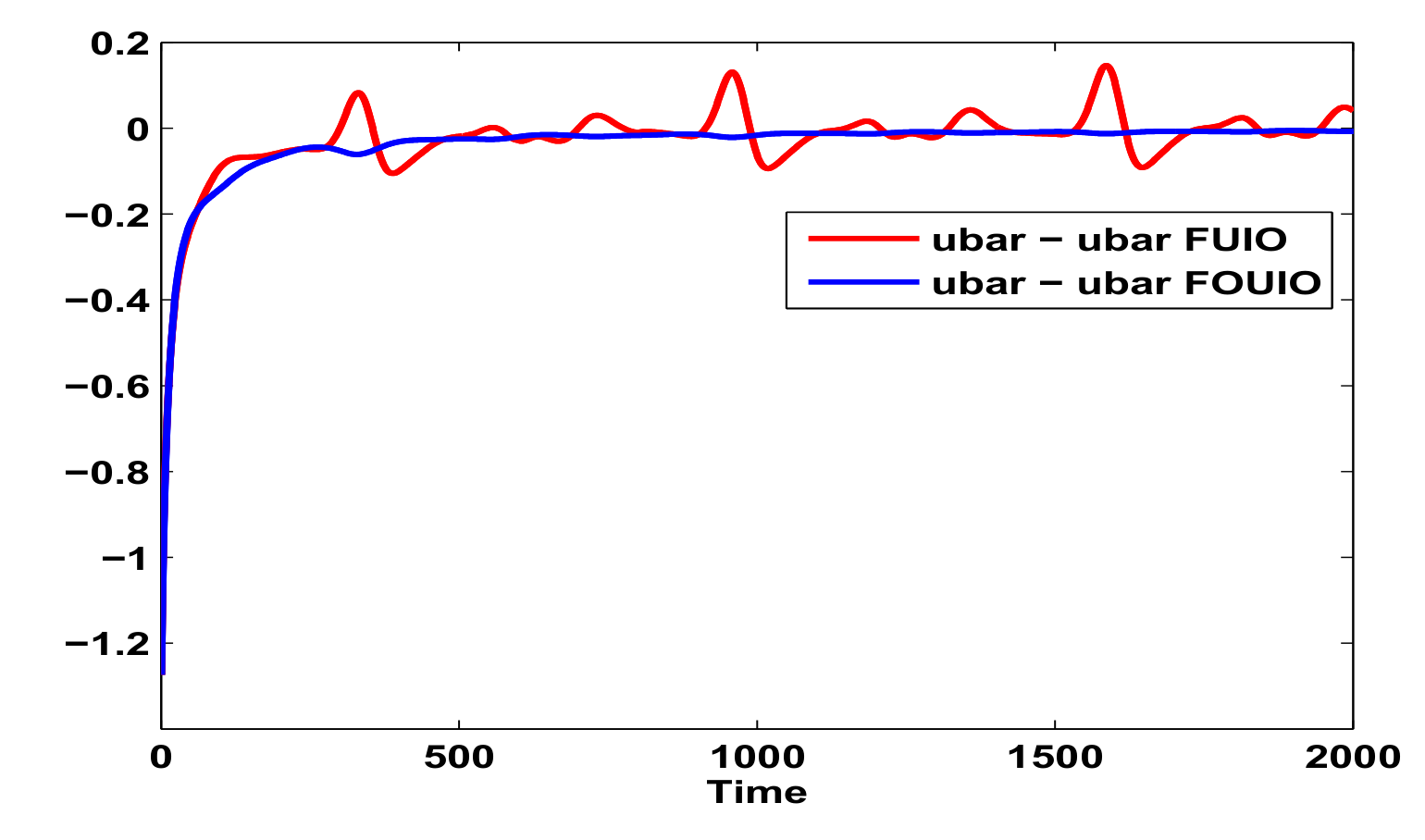
Example and Simulation Results

Consider the FOTS model (8), which is defined as follows:

$$\left\{\begin{array}{c}{}_{t_0}{D}_t^{\alpha }\widehat{x}\left(t\right)={\displaystyle \sum _{i=0}^M}{h}_i\left(x\left(t\right)\right)\left[A_{i}x\left(t\right)+B_{i}u\left(t\right)+F_i\overline{u}\left(t\right)\right],\hfill \\ y\left(t\right)=Cx\left(t\right)+G\overline{u}\left(t\right),\hfill \end{array}\right.$$

(68)

where: $A_1=\left[\begin{array}{ccc}-2& 1& 1\\ 1& -3& 0\\ 2& 1& -4\end{array}\right]$, $A_2=\left[\begin{array}{ccc}-3& 2& -2\\ 5& -3& 0\\ 0.5& 0.5& -4\end{array}\right]$, $B_1=\left[\begin{array}{c}1\\ 0.3\\ 0.5\end{array}\right]$, $B_2=\left[\begin{array}{c}0.5\\ 1\\ 0.25\end{array}\right]$, $C=\left[\begin{array}{ccc}1& 1& 1\\ 1& 0& 1\end{array}\right]$, $F_1=\left[\begin{array}{c}0.5\\ -1\\ 0.25\end{array}\right]$, $F_2=\left[\begin{array}{c}-1\\ 0.52\\ 1\end{array}\right]$, $G=\left[\begin{array}{c}0.9\\ 0.9\end{array}\right].$

The activation functions are chosen in the form:

$$\left\{\begin{array}{c}{h}_1\left(x\right)=\frac{1-tanh\left(x_1\right)}{2},\hfill \\ h_2\left(x\right)=1-h_1\left(x\right)=\frac{1+tanh\left(x_1\right)}{2}.\hfill \end{array}\right.$$

(69)

Two cases are considered for simulation, the first one in the absence of unknown inputs (unknown inputs are null), and the second one in the presence of unknown inputs. The unknown input considered is accompanied by an additive noise. To have a treatment close to reality, the initial values of the system are chosen non-null, but the initial values of the two unknown input observers are chosen equal to zero.

The outputs and the states of the FOTS system with their estimations given by the fuzzy integer and fractional order unknown input observers, and the unknown inputs and their estimates will be compared and analyzed.

Case 1: Absence of unknown input.

At first, the case of the absence of unknown inputs (unknown inputs are null) will be evaluated. Figure 1 shows the two outputs of the considered FOTS system $(y{s}_1,y{s}_2)$, the outputs estimated by the FOUIO $(y{o}_1,y{o}_2)$ and the fractional order unknown input observer (FOUIO) $(yf{o}_1,yf{o}_2)$ in the absence of unknown inputs. Figure 2 shows the outputs estimation error (a and b) in the absence of unknown inputs $(y{s}_1-y{o}_1,y{s}_2-y{o}_2)$ and $(y{s}_1-yf{o}_1,y{s}_2-yf{o}_2)$. The two Figure 1 and Figure 2 show that the FOUIO gives better output estimation for the considered system. The decreased quality of the output estimation at the moment $t=0$ is because of the choice of the initial values.

Figure 3 presents the states of the FOTS system $(x{s}_1,x{s}_2,x{s}_3)$ and their estimations given by the FUIO $(x{o}_1,x{o}_2,x{o}_3)$ and the FOUIO $(xf{o}_1,xf{o}_2,xf{o}_3)$ in the absence of unknown inputs. Figure 4 shows the state estimation errors (a and b) in the absence of unknown inputs $(x{s}_1-x{o}_1,x{s}_2-x{o}_2,x{s}_3-x{o}_3)$ and $(x{s}_1-xf{o}_1,x{s}_2-xf{o}_2,x{s}_3-xf{o}_3)$. The two Figure 3 and Figure 4 show that the fuzzy observer with unknown inputs gives a better state estimation of the FOTS system. The decreased quality of the state estimation at the moment $t=0$ is because of the choice of the initial values.

Now, the case of the presence of unknown inputs will be evaluated.

Case 2: Presence of unknown input and measurement noise simultaneously.

Figure 5 shows the outputs of the FOTS system $(y{s}_1,y{s}_2)$, and their estimations given by the FUIO $(y{o}_1,y{o}_2)$ and the fuzzy FOUIO $(yf{o}_1,yf{o}_2)$ in the presence of unknown inputs. Figure 6 shows the outputs estimation error (a and b) in the presence of unknown inputs $(y{s}_1-y{o}_1,y{s}_2-y{o}_2)$ and $(y{s}_1-yf{o}_1,y{s}_2-yf{o}_2)$. The two Figure 5 and Figure 6 show that the FOUIO gives a better output estimation for the FOTS system. The decreased quality of the outputs estimation at the moment $t=0$ is because of the choice of the initial values.

Figure 7 presents the states of the FOTS system $(x{s}_1,x{s}_2,x{s}_3)$ and their estimations given by the FUIO $(x{o}_1,x{o}_2,x{o}_3)$ and the FOUIO $(xf{o}_1,xf{o}_2,xf{o}_3)$ in the presence of unknown inputs. Figure 8 shows the state estimation errors (a and b) in the presence of unknown inputs $(x{s}_1-x{o}_1,$$x{s}_2-x{o}_2,$$x{s}_3-x{o}_3)$ and $(x{s}_1-xf{o}_1,$$x{s}_2-xf{o}_2,$$x{s}_3-xf{o}_3)$. The two Figure 7 and Figure 8 show that the FOUIO gives a better state estimation for the FOTS system. The decreased quality of the state estimation at the moment $t=0$ is because of the choice of the initial values.

Analyzing the convergence conditions of the proposed FOUIO, if the condition (23) on the term $\omega \left(t\right)$ is not satisfied or the value of the constant $\delta$ is very important (impossibility of finding a solution with Theorem 1, Theorem 2) offers the possibility of designing the observer with unknown input.

Figure 9 shows the considered unknown input with normal noise (ubar), their estimations given by the FUIO (ubar FUIO), FOUIO (ubar FOUIO) and the unknown input without noise (ubar without noise).

Figure 10 shows the unknown input estimation errors (ubar-ubar FUIO, ubar-ubar FOUIO).

The two Figure 9 and Figure 10 show that the FOUIO gives a better unknown input estimation of the FOTS system, but it cannot be decoupled from the noise. The decreased quality of the unknown input estimation at the moment $t=0$ is because of the choice of the initial values.

In the presence of adding random measurement noises bounded by 0.01, the unknown input estimated based on the proposed observer is noisy. Indeed, the presence of measurement noise, at high frequency, decreases the quality of reconstruction of the unknown input.

7. Conclusions

In this paper, a new approach is proposed for designing a fractional order Takagi–Sugeno unknown input observer for a nonlinear system described by FOTS models with UPV. The first step is to rewrite the FOTS system in the form of a disturbed equivalent FOTS and with measurable premise variables. After that, two cases are considered; the first one uses the hypothesis that the perturbation, which appears after rewriting the FOTS model, verifies a Lipschitz condition, while the second one does not use this hypothesis. In this second case, another method is developed and based on an $L_2$ approach. The convergence conditions of the proposed observers are given in the form of linear matrix inequalities (LMI) that can be easily solved with conventional digital tools.

The obtained results show that a good convergence of the outputs and the state estimation errors is observed using the new proposed FOUIO. The state of the system can be estimated even in the presence of an unknown input varying rapidly since it is totally decoupled from the state. An improvement in the dynamics of the proposed observer is possible by placing the poles.

In future work, it would be interesting to study the decoupling of the noise and the estimation of the unknown inputs using the augmented systems.

References

1. Machado, J.T.; Kiryakova, V.; Mainardi, F. Recent history of fractional calculus. Commun. Nonlinear Sci. Numer. Simul. 2011, 16, 1140–1153. [Google Scholar] [CrossRef] [Green Version]
2. Oldham, K.B.; Spanier, J. The Fractional Calculus, Theory and Applications of Differentiation and Integration of Arbitrary Order; Academic Press: New York, NY, USA, 1974. [Google Scholar]
3. Miller, K.S.; Ross, B. The Fractional Calculus, an Introduction to the Fractional Calculus and Fractional Deferential Equations; John Wiley & Sons Inc.: New York, NY, USA, 1993. [Google Scholar]
4. George, A.; Argyros, I.K. Intelligent Numerical Methods: Applications to Fractional Calculus; Springer International Publishing: Cham, Switzerland, 2016; Volume 624. [Google Scholar]
5. Li, W.; Zhao, H.M. Rational function approximation for fractional order differential and integral operators. Acta Autom. Sin. 2011, 37, 999–1005. [Google Scholar]
6. Xe, D.Y.; Zhao, C.N.; Chen, Y.Q. Robust control for fractional order four-wing hyperchaotic system using LMI. In Proceedings of the IEEE Conference on Mechatronics and Automation, Luoyang, China, 25–28 June 2006; pp. 1043–1048. [Google Scholar]
7. Li, C.L.; Su, K.L.; Zhang, J.; Wei, D.Q. Rational function approximation for fractional order differential and integral operators. Opt. Int. J. Light Electron Opt. 2013, 124, 5807–5810. [Google Scholar] [CrossRef]
8. Yuan, J.; Shi, B.; Ji, W.Q. Adaptive sliding mode control of a novel class of fractional chaotic systems. Adv. Math. Phys. 2013, 2013, 6709. [Google Scholar] [CrossRef]
9. Li, W.; Peng, C.; Wang, Y. Frequency domain subspace identification of commensurate fractional order input time delay systems. Int. J. Control. Autom. Syst. 2011, 9, 310–316. [Google Scholar]
10. Vinagre, B.M.; Podlubny, I.; Dorcak, L.; Feliu, V. On fractional PID controllers: A frequency domain approach. In Proceedings of the IFAC Workshop on Digital Control: Past, Present and Future of PID Control, Terrasa, Spain, 5–7 April 2000; pp. 53–58. [Google Scholar]
11. Aldair, A.A.; Wang, W.J. Design of fractional order controller based on evolutionary algorithm for a full vehicle nonlinear active suspension systems. Int. J. Control. Autom. 2010, 3, 33–46. [Google Scholar]
12. Ostalczyk, P. Discrete Fractional Calculus: Applications in Control and Image Processing. In Series in Computer Vision; World Scientific Publishing Co.: Singapore, 2016; Volume 4. [Google Scholar]
13. Mozyrska, D.; Wyrwas, M. The Z-transform method and delta type fractional difference operators. Discret. Dyn. Nat. Soc. 2015, 2–3, 1–12. [Google Scholar] [CrossRef]
14. Das, S. Functional Fractional Calculus for System Identification and Controls; Springer: Berlin/Heidelberg, Germany, 2008. [Google Scholar]
15. Ibrir, S. Robust state estimation with q-integral observers. In Proceedings of the American Control Conference, Boston, MA, USA, 30 June–2 July 2004; pp. 3466–3471. [Google Scholar]
16. Farges, C.; Moze, M.; Sabatier, J. Pseudo-state feedback stabilization of commensurate fractional order systems. Automatica 2010, 46, 1730–1734. [Google Scholar] [CrossRef]
17. Stanisławski, R.; Rydel, M.; Latawiec, K.J. Modeling of discrete-time fractional-order state space systems using the balanced truncation method. J. Frankl. Inst. 2017, 354, 3008–3020. [Google Scholar] [CrossRef]
18. Doye, I.; Darouach, M.; Voos, H.; Zasadzinsk, M. Design of unknown input fractional-order observer for fractional-order systems. Int. J. Appl. Math. Comput. Sci. 2013, 23, 491–500. [Google Scholar] [CrossRef]
19. Wei, Y.H.; Sun, Z.Y.; Hu, Y.S.; Wang, Y. On fractional order adaptive observer. Int. J. Autom. Comput. 2015, 12, 664–670. [Google Scholar] [CrossRef] [Green Version]
20. Sabatier, J.; Farges, C.; Merveillaut, M.; Feneteau, L. On Observability and Pseudo State Estimation of Fractional Order Systems. Eur. J. Control. 2012, 18, 260–271. [Google Scholar] [CrossRef]
21. Safarinejadian, B.; Asad, M.; Sha Sadeghi, M. Simultaneous state estimation and parameter identification in linear fractional order systems using colored measurement noise. Int. J. Control. 2016, 89, 2277–2296. [Google Scholar] [CrossRef]
22. Li, F.; Wu, R.; Liang, S. Observer-based state estimation for non-linear fractional systems. Int. J. Dyn. Syst. Differ. Equ. 2015, 5, 322–335. [Google Scholar] [CrossRef]
23. Fuli, Z.; Hui, L.; Shouming, Z. State estimation based on fractional order sliding mode observer method for a class of uncertain fractional-order nonlinear systems. Signal Process. 2016, 127, 168–184. [Google Scholar]
24. Kong, S.; Saif, M.; Liu, B. Observer design for a class of nonlinear fractional-order systems with unknown input. J. Frankl. Inst. 2017, 354, 5503–5518. [Google Scholar] [CrossRef]
25. Djeghali, N.; Djennoune, S.; Bettayeb, M.; Ghanes, M.; Barbot, J.P. Observation and sliding mode observer for nonlinear fractional-order system with unknown input. ISA Trans. 2016, 63, 1–10. [Google Scholar] [CrossRef]
26. Ding, B.; Sun, H.; Yang, P. Further studies on LMI based relaxed stabilization conditions for nonlinear systems in Takagi–Sugeno’s form. Automatica 2006, 42, 503–508. [Google Scholar] [CrossRef]
27. Kruszewski, A.; Wang, R.; Guerra, T.M. Nonquadratic stabilization conditions for a class of uncertain nonlinear discrete time TS fuzzy models: A new approach. IEEE Trans. Autom. Control. 2008, 53, 606–611. [Google Scholar] [CrossRef]
28. N’Doye, I.; Darouach, M.; Zasadzinski, M.; Radhy, N.E. Robust stabilization of uncertain descriptor fractional-order systems. Automatica 2013, 49, 1907–1913. [Google Scholar] [CrossRef]
29. Lu, J.G.; Chen, Y.Q. Robust stability and stabilization of fractional-order interval systems with the fractional order α: The case 0 < α < 1. IEEE Trans. Autom. Control. 2010, 55, 152–158. [Google Scholar]
30. Trigeassou, J.; Maamri, N.; Sabatier, J.; Oustaloup, A. A Lyapunov approach to the stability of fractional differential equations. Signal Process. 2011, 91, 437–445. [Google Scholar] [CrossRef]
31. Yu, W.; Li, Y.; Wen, G.; Yu, X.; Cao, J. Observer design for tracking consensus in second-order multi-agent systems: Fractional order less than two. IEEE Trans. Autom. Control. 2017, 62, 894–900. [Google Scholar] [CrossRef]
32. Park, J.H.; Park, T.S.; Kim, S.H. Approximation-Free Output-Feedback Non-Backstepping Controller for Uncertain SISO Nonautonomous Nonlinear Pure-Feedback Systems. Mathematics 2019, 7, 456. [Google Scholar] [CrossRef]
33. Faieghi, M.; Mashhadi, S.K.M.; Baleanu, D. Sampled-data nonlinear observer design for chaos synchronization: A Lyapunov-based approach. Commun. Nonlinear Sci. Numer. Simul. 2014, 19, 2444–2453. [Google Scholar] [CrossRef]
34. Zhang, X.; Ding, F.; Xu, L.; Alsaedi, A.; Tasawar, H. A Hierarchical Approach for Joint Parameter and State Estimation of a Bilinear System with Autoregressive Noise. Mathematics 2019, 7, 356. [Google Scholar] [CrossRef]
35. Ibrir, S.; Bettayeb, M. New sufficient conditions for observer-based control of fractional-order uncertain systems. Automatica 2015, 59, 216–223. [Google Scholar] [CrossRef]
36. Song, C.; Fei, S.; Cao, J.; Huang, C. Robust Synchronization of Fractional-Order Uncertain Chaotic Systems Based on Output Feedback Sliding Mode Control. Mathematics 2019, 7, 599. [Google Scholar] [CrossRef]
37. Liu, S.; Dong, X.; Zhang, Y. A New State of Charge Estimation Method for Lithium-Ion Battery Based on the Fractional Order Model. IEEE Access 2019, 7, 122949–122954. [Google Scholar] [CrossRef]
38. Shi, S.L.; Li, J.X.; Fang, Y.M. Fractional-disturbance-observer-based Sliding Mode Control for Fractional Order System with Matched and Mismatched Disturbances. Int. J. Control. Autom. Syst. 2019, 17, 1184–1190. [Google Scholar] [CrossRef]
39. Trinh, H.; Huong, D.C.; Nahavandi, S. Observer design for positive fractional-order interconnected time-delay systems. Trans. Inst. Meas. Control. Publ. 2018, 41, 378–391. [Google Scholar] [CrossRef]
40. Dabiri, A.; Butcher, E. Optimal observer-based feedback control for linear fractional-order systems with periodic coefficients. J. Vib. Control. 2019, 25, 1379–1392. [Google Scholar] [CrossRef]
41. Kong, S.; Saif, M.; Cui, G. Estimation and Fault Diagnosis of Lithium-Ion Batteries: A Fractional-Order System Approach. Math. Probl. Eng. 2018, 8705363, 1–12. [Google Scholar] [CrossRef]
42. Yang, B.; Yu, T.; Shu, H.; Zhu, D.; Sang, Y.; Jiang, L. Passivity-based fractional-order sliding-mode control design and implementation of grid-connected photovoltaic systems. J. Renew. Sustain. Energy 2018, 10, 43701. [Google Scholar] [CrossRef]
43. Chadli, M.; Karimi, H.R. Robust observer design for unknown inputs Takagi–Sugeno models. IEEE Trans. Fuzzy Syst. 2013, 21, 158–164. [Google Scholar] [CrossRef]
44. Liu, S.; Li, X.; Wang, H.; Yan, J. Adaptive fault estimation for T-S fuzzy systems with unmeasurable premise variables. Adv. Differ. Equ. 2018, 105. [Google Scholar] [CrossRef]
45. Takagi, T.; Sugeno, M. Fuzzy identification of systems and its applications to modeling and control. IEEE Trans. Syst. Man Cybern. Part B Cybern. 1985, SMC-15, 116–132. [Google Scholar] [CrossRef]
46. Krokavec, D.; Filasova, A. On observer design methods for a class of Takagi Sugeno fuzzy systems. In Proceedings of the Third International Conference on Advanced Information Technologies & Applications, Dubai, UAE, 7–8 November 2014; pp. 279–290. [Google Scholar]
47. Djeddi, A.; Harkat, M.F.; Soufi, Y. A New Approach for State Estimation of Uncertain Multiple model with Unknown Inputs. Application to Sensor Fault Diagnosis. Mediterr. J. Meas. Control. 2016, 12, 537–545. [Google Scholar]
48. Chadli, M.; Guerra, T.M. LMI solution for robust static output feedback control of Takagi–Sugeno fuzzy models. IEEE Trans. Fuzzy Syst. 2012, 20, 1060–1065. [Google Scholar] [CrossRef]
49. Oukacine, S.; Djamah, T.; Djennoune, S.; Mansouri, R.; Bettayeb, M. Multi-model identification of a fractional nonlinear system. IFAC Proc. 2013, 46, 48–53. [Google Scholar] [CrossRef]
50. Junmin, L.; Yuting, L. Robust Stability and Stabilization of Fractional Order Systems Based on Uncertain Takagi–Sugeno Fuzzy Model With the Fractional Order 1 ≤ ν < 2. ASME J. Comput. Nonlinear Dyn. 2013, 8, 41005. [Google Scholar]
51. Gao, Z.; Liao, X. Observer-based fuzzy control for nonlinear fractional-order systems via fuzzy T-S models: The 1 < α < 2 case. In Proceedings of the 19th World Congress, The International Federation of Automatic Control, Cape Town, South Africa, 24–29 August 2014. [Google Scholar]
52. Ichalal, D.; Marx, B.; Mammar, S.; Maquin, D.; Ragot, J. How to cope with unmeasurable premise variables in Takagi–Sugeno observer design: Dynamic extension approach. Eng. Appl. Artif. Intell. 2018, 67, 430–435. [Google Scholar] [CrossRef]
53. Shantanu, D. Functional Fractional Calculus, 2nd ed.; Springer: Berlin/Heidelberg, Germany, 2011. [Google Scholar]
54. Petras, I. Fractional-Order Nonlinear Systems Modeling, Analysis and Simulation; Higher Education Press: Beijing, China; Springer: Berlin/Heidelberg, Germany, 2011. [Google Scholar]
55. Akhenak, A.; Chadli, M.; Ragot, J.; Maquin, D. Estimation of state and unknown inputs of a nonlinear system represented by a multiple model. IFAC Proc. Vol. 2004, 37, 385–390. [Google Scholar] [CrossRef]
56. Boyd, S.; El Ghaoui, L.; Feron, E.; Balakrishnan, V. Linear Matrix Inequalities in System and Control Theory; SIAM: Philadelphia, PA, USA, 1994. [Google Scholar]
Figure 1. Outputs of the fractional-order Takagi–Sugeno (FOTS) system and its estimation by FOUIO and fractional order unknown input observer (FOUIO) in a free of fault case.
Mathematics 07 00984 g001
Figure 2. Output estimation Error in a free of fault case. (a) Error output estimation of the FOTS system by FUIO in a free of fault case. (b) Error output estimation of the FOTS system by FOUIO in a free of fault case.
Mathematics 07 00984 g002
Figure 3. State of the FOTS system and its estimation by FUIO and FOUIO in a free of fault case.
Mathematics 07 00984 g003
Figure 4. State estimation error in free of fault case. (a) State estimation error between the FOTS system and FUIO in a free of fault case. (b) State estimation error between the FOTS system and FOUIO in a free of fault case.
Mathematics 07 00984 g004
Figure 5. Outputs for the FOTS system and its estimation by FUIO and FOUIO in a faulty case.
Mathematics 07 00984 g005
Figure 6. Output for error estimation faulty case. (a) Outputs for error estimation between the FOTS system and FUIO in a faulty case. (b) Outputs error estimation between the FOTS system and FOUIO in a faulty case.
Mathematics 07 00984 g006
Figure 7. State estimation for the FOTS system and its estimations by FUIO and FOUIO in a faulty case.
Mathematics 07 00984 g007
Figure 8. Output estimation error in faulty case. (a) State estimation error between the FOTS system and FUIO in a faulty case. (b) State estimation error between the FOTS system and FOUIO in a faulty case.
Mathematics 07 00984 g008
Figure 9. Unknown input and their estimations.
Mathematics 07 00984 g009
Figure 10. Unknown input errors estimation.
Mathematics 07 00984 g010