Optimal Control of a PDE Model of an Invasive Species in a River

Abstract

Managing invasive species in rivers can be assisted by appropriate adjustment of flow rates. Using a partial differential equation (PDE) model representing an invasive population in a river, we investigate controlling the water discharge rate as a management strategy. Our goal is to see how controlling the water discharge rate will affect the invasive population, and more specifically how water discharges may force the invasive population downstream. We complete the analysis of a flow control problem, which seeks to minimize the invasive population upstream while minimizing the cost of this management. Using an optimality system, consisting of our population PDE, an adjoint PDE, and corresponding optimal control characterization, we illustrate some numerical simulations in which parameters are varied to determine how far upstream the invasive population reaches. We also change the river’s cross-sectional area to investigate its impact on the optimal control.

1. Introduction

The need to develop methods for managing invasive species in rivers is growing [1,2,3], and modelling can give insight into management strategies. Jacobsen et al. [4], Jin and Lewis [5,6], and Gagnon et al. [7] used integrodifference models to represent such populations in rivers. With a more realistic model, Jacobsen et al. concluded that longer stream length and lower flow rates increase the chance of a species persisting while higher flow streams must be even longer to maintain persistence [4]. They also showed that flow velocity variability can produce persistence similar to the mean velocity [4]. Jin and Lewis [5,6] also conducted a theoretical analysis using integrodifference equations assuming periodicity with respect to time. In 2011, they first explored how the critical domain size would affect the species persistence and determined that a periodic dispersal kernel and a weighted time-averaged dispersal kernel have the same effect. However, this only holds for the estimation of the critical domain size [5]. In 2012, Jin and Lewis [6] studied spreading speeds for the same integrodifference equations in [5]. Jin and Lewis again found that the periodic dispersal kernel and the weighted time-averaged dispersal kernel both yield the same spreading speeds. Once again, this only applied for the spreading speeds, and there is no proof that the dynamics of the systems are the same [6]. In [7], Gagnon et al. took an applied approach having a specific species, Codium fragile. Gagnon et al. focused on wind-driven spread of floating fragments of this algae. They found that prevalent winds were vital in determining the spreading speeds as well as the fragmentation into non-buoyant and buoyant pieces was the most important feature in determining spread [7].

In a recent paper, Jin et al. built a reaction–diffusion partial differential equation (PDE) model to better represent a population in a river by using not just the population growth, but how the river itself changes over time [8]. The idea was that this new model would better represent a population trying to move up a river. Clifford et al. [9] discussed how water flow affects the ecology of the river and the shift from focusing purely on river flow dynamics to how these flow dynamics create various habitats [9]. Huang et al. [10] used a PDE system to examine how a species that usually lives in the benthic layer of a river may move in the stream using drift. They used three values to measure the persistence of a species in the river and found that the net reproductive rate determined if a population could persist in the river or not [10]. In a later paper in 2017, Jin et al. [11] explored how the cross-sectional area of a river would affect whether the population persisted. Assuming the meandering rivers are periodic, the cross-sectional area changes over time [11]. They found that increasing growth rates increases the chance of persistence by the population and allows for spreading both up and downstream while increasing flow spread decreases the chance of persistence and upstream spread but increases downstream spread.

Jin et al. [8] explored simpler forms of the models by setting the cross-sectional area and water discharge to constant values to see how a population would move in the stream. They began with traveling waves in constant environments and temporally or spatially heterogeneous environments. To see the effect on the population’s movement upstream, Jin et al. then varied the water discharge and cross-sectional area between two time periods to illustrate a seasonal period of summer versus winter. The water discharge and cross-sectional area in the summer are two values, and in the winter are other values. To investigate time varying flows and corresponding management, we use optimal control theory on the water flow discharge to control the movement of an invasive species upstream.

We are interested in modeling an invasive species (like carp) which moves upstream. To manage an invasive species in a downstream position in a river, one needs an action to keep that species from moving upstream. Current methods to prevent further expansion include electric fences or nets in the river [1]. In addition, adjusting the flow rate via dams or water release mechanisms may be a reasonable containment mechanism. Poff and Zimmerman [12] mention that extreme changes in river flow can affect a populations survival success in a habitat. They discuss flows changing due to climate and controlling runoff by catchment [12]. Using the Jin et al. [8] model in our work, we choose the water discharge “flow” function to affect the invasive species movement upstream. Taking the advection coefficient as a time varying control function, we will be utilizing optimal control theory to analyze this model and this management mechanism to contain the species downstream.

In the following sections, we first formulate the problem and describe the terms of the PDE model. We define the weak solution and the solution space. We then describe the control set and the objective functional to be minimized. Using a priori bounds on the state in the weak solution space, we prove the existence of the optimal control. Then, we prove differentiability of the control-to-state solution map while giving the sensitivity system leading to the adjoint system. We differentiate the objective functional and derive an optimal control characterization using the sensitivity and adjoint systems. Finally, we present some numerical simulations to show the effects of our optimal control on the movement of the population. Specifically, we illustrate how the population moves upstream with and without control.

2. Optimal Control Problem Formulation

We use the model adapted from Jin et al. [8]. To formulate our state PDE and corresponding optimal control problem for the weak solutions, our solution spaces are $V=L^2(0,T;H_{\left\{0\right\}}^1(0,L))$ and $V^{*}=L^2(0,T;{(H_{\left\{0\right\}}^1(0,L))}^{*})$, where the subscript $\left\{0\right\}$ indicates that the functions vanish at $x=0$.

Definition 1.

A function $N\in V\cap L^{\infty }((0,T)\times (0,L))$ with $N_t\in V^{*}$ is a weak solution of the state PDE:

$$\begin{array}{cc}\hfill & N_t=-A_t(x,t)\frac{N}{A(x,t)}+\frac{1}{A(x,t)}{\left(D(x,t)A(x,t)N_x\right)}_x-\frac{Q\left(t\right)}{A(x,t)}{N}_x+rN\left(1-\frac{N}{K}\right)\hfill \\ \hfill & N(0,t)=0on(0,T),x=0,\hfill \\ \hfill & N_x(L,t)=0on(0,T),x=L,\hfill \\ \hfill & N(x,0)=N_0\left(x\right)on(0,L),t=0\hfill \end{array}$$

(1)

in $\mathsf{\Lambda }=(0,L)\times (0,T)$, if

$${\int }_0^T\langle N_t,\varphi \rangle dt+{\int }_0^T{\int }_0^L\left(A_t\frac{N\varphi }{A}+DA{N}_x{\left(\frac{\varphi }{A}\right)}_x+\frac{Q}{A}{N}_x\varphi -rN\varphi \left(1-\frac{N}{K}\right)\right)dxdt=0$$

for all $\varphi \in V$, where $\langle ,\rangle$ in the integrand denotes the duality $H_{\left\{0\right\}}^1\left(0,L\right),H_{\left\{0\right\}}^1{\left(0,L\right)}^{*}$.

The state $N(x,t)$ represents the population density in the river, $A(x,t)$ is the cross-sectional area of the river at location x at time t, $D(x,t)$ is the diffusion coefficient, r is the population intrinsic growth rate, and K is the carrying capacity. The control function $Q\left(t\right)$ represents the water discharge rate. An important note is that the location $x=0$ is upstream while $x=L$ is downstream. For our boundary conditions, at upstream where $x=0$, we assume no population is initially there, as they are invading by moving from downstream to upstream. Likewise, at downstream, $x=L$, we assume no flux, meaning the population is not increased from an outside source. To simplify the calculations, the model uses a one-dimensional, spatial domain corresponding to the length of the river with the assumption of homogeneous mixing in any cross-sectional area.

Our goal is to control the water discharge rate $Q\left(t\right)$ to prevent an invasive species from moving upstream. Our control set for $0<m\le M$ is

$$U=\{Q\in L^{\infty }(0,T)|m\le Q\left(t\right)\le M\}.$$

Because of the damming of rivers, $Q\left(t\right)$ is bounded above by some value M and bounded below by m positive since water discharge by definition must be positive. We assume we can fully control the water discharge rate by controlling how much water moves through a dam. Note that $Q\left(t\right)$ is not a function of space, but just time. The idea explored in Jin et al. is that the water discharge rate being higher during certain seasons and lower in others affects the population level at various locations [8].

Our objective functional which we intend to minimize is:

$$J\left(Q\right)={\int }_0^T{\int }_0^{L}W\left(x\right)N(x,t)dxdt+{\int }_0^TϵQ^2\left(t\right)dt,$$

where $ϵ>0$ is small. The coefficient $W\left(x\right)$ is a weight function that is large at $x=0$ and small at $x=L$ since our goal is to keep the population downstream (at $x=L$). The first integration term seeks to minimize the size of the invasive species with an emphasis on keeping the invader downstream (due to the weight function) by decreasing N near $x=L$. The $Q^2\left(t\right)$ term seeks to minimize the cost of effort needed to stop the species from moving upstream with an $ϵ$ coefficient to keep it small. Thus, the term with $W\left(x\right)N(x,t)$ should dominate the objective functional. We seek $Q^{*}\in U$ such that

$$J\left(Q^{*}\right)=\underset{Q\in U}{inf}J\left(Q\right).$$

Assuming A is a $C^1$ function and D is a continuous function on our domain, we make the following additional assumptions:

$$r>0,K>0,$$

$$0<m\le Q\left(t\right)\le M,$$

$$0<{ϵ}_A\le A(x,t)\le M_A,$$

$$|A_x(x,t)|\le M_B,\left|A_t(x,t)\right|\le M_C,$$

$$0<{ϵ}_D\le D(x,t)\le M_D,$$

$$0\le N_0(x,t)\le M_1.$$

To solve the optimal control problem for a given $Q\in U$, we need the existence of a unique weak state solution to (1), and this solution must be non-negative and bounded above. The corresponding two theorems follow from results as in [13,14].

Theorem 1 (Positivity and Existence of State Solution).

Given $N_0$ non-negative, $L^{\infty }\left(0,L\right)$ bounded and in $H_{\left\{0\right\}}^1\left(0,L\right)$, then, for each $Q\in U$, there is a unique non-negative weak solution $N=N\left(Q\right)$ of tjhe state PDE (1) with $0\le N(x,t)\le C$, where C holds for all $Q\in U$.

Theorem 2 (A priori estimates).

There exists positive constants ${\alpha }_1$ and ${\alpha }_2$ such that, for any $Q\in U,$ and $N\in V\cap L^{\infty }\left(\mathsf{\Lambda }\right)$ where $N_t\in L^2(0,T;{(H_{\left\{0\right\}}^1(0,L))}^{*})$, the weak solution of the PDE corresponding to Q with $N\ge 0$ a.e. satisfies

$$\left({\int \int }_{\mathsf{\Lambda }}{N}_x^{2}dxdt+{\int \int }_{\mathsf{\Lambda }}{N}^{2}dxdt\right)\le {\alpha }_1$$

(2)

and ${∥N_t∥}_{V^{*}}\le {\alpha }_2.$

We denote the weak solution of the state PDE (1) corresponding to control Q as $N\left(Q\right)$.

Theorem 3 (Existence of Optimal Control).

There exists an optimal control, $Q^{*}\in U,$ satisfying

$$J\left(Q^{*}\right)=\underset{Q\in U}{inf}J\left(Q\right).$$

Proof. 

We choose a minimizing sequence $\left\{Q^n\right\}\subset U$ with $n=1,2,3,\dots$ such that

$$\underset{n\to \infty }{lim}J\left(Q^n\right)=\underset{Q\in U}{inf}J\left(Q\right)$$

and $N^n=N\left(Q^n\right)$ the corresponding solution to tje state PDE (1). By the a priori estimates in Theorem 2, there exists $N^{*}\in V\bigcap L^{\infty }\left(\left(0,T\right)\times \left(0,L\right)\right)$, with $N_t^{*}\in V^{*}$, and $Q^{*}\in U$ such that, on a subsequence, these weak convergences hold:

$$\begin{array}{cc}\hfill N^n& \rightharpoonup N^{*}\mathrm{in}V,\hfill \\ \hfill N_t^n& \rightharpoonup N_t^{*}\mathrm{in}{V}^{*},\hfill \\ \hfill Q^n& \rightharpoonup Q^{*}\mathrm{in}{L}^2\left(\left(0,T\right)\times \left(0,L\right)\right).\hfill \end{array}$$

(3)

We must show that $N^{*}=N\left(Q^{*}\right)$, where $N^{*}$ is the population solution associated with $Q^{*}$. Using the compactness result in [15] coupled with the convergences in (3), we obtain this strong $L^2$ convergence,

$$N^n\to N^{*}\mathrm{in}{L}^2\left(\left(0,T\right)\times \left(0,L\right)\right).$$

Now, we must show that $Q^{*}$ is an optimal control and that $N^{*}=N\left(Q^{*}\right)$. Using the convergences in (3) and the $L^{\infty }$ bounds on Q, the convergences above give limits for these terms:

$$\begin{array}{cc}\hfill & {\int }_0^T\langle N_t^n,\varphi \rangle dt\rightharpoonup {\int }_0^T\langle N^{*},\varphi \rangle dt\hfill \\ \hfill & {\int }_0^T{\int }_0^L\frac{A_t}{A}{N}^n\varphi dxdt\to {\int }_0^T{\int }_0^L\frac{A_t}{A}{N}^{*}\varphi dxdt\hfill \\ \hfill & {\int }_0^T{\int }_0^{L}DA{N}_x^n{\left(\frac{\varphi }{A}\right)}_{x}dxdt\rightharpoonup {\int }_0^T{\int }_0^{L}DA{N}_x^{*}{\left(\frac{\varphi }{A}\right)}_{x}dxdt\hfill \\ \hfill & {\int }_0^T{\int }_0^L-r{N}^n\varphi dxdt\to {\int }_0^T{\int }_0^L-r{N}^{*}\varphi dxdt\hfill \\ \hfill & {\int }_0^T{\int }_0^L\frac{r\varphi }{K}{\left(N^n\right)}^{2}dxdt\to {\int }_0^T{\int }_0^L\frac{r\varphi }{K}{\left(N^{*}\right)}^{2}dxdt.\hfill \end{array}$$

To handle a term with $Q^n$ and $N_x^n$, integrating by parts and rearranging gives

$$\begin{array}{cc}\hfill {\int }_0^T{\int }_0^L\frac{1}{A}& \left(Q^n{N}_x^n-Q^{*}{N}_x^{*}\right)\varphi dxdt\hfill \\ \hfill & =-{\int }_0^T{\int }_0^L{Q}^n{\left(\frac{\varphi }{A}\right)}_x\left(N^n-N^{*}\right)dxdt-{\int }_0^T{\int }_0^L{N}^{*}{\left(\frac{\varphi }{A}\right)}_x\left(Q^n-Q^{*}\right)dxdt\hfill \\ \hfill & +{\int }_0^T\frac{Q^n\varphi }{A}\left(N^n-N^{*}\right)\left(L,t\right)dt+{\int }_0^T\frac{N^{*}\varphi }{A}\left(Q^n-Q^{*}\right)\left(L,t\right)dt.\hfill \end{array}$$

(4)

By the Cauchy–Schwartz inequality, the strong convergence of $\left\{N^n\right\}$, $\varphi$ being in $L^2$ and the $L^{\infty }$ bounds on $\left\{Q^n\right\}$, the first and third terms of Equation (4) give

$$\begin{array}{cc}\hfill \underset{n\to \infty }{lim}& \left|-{\int }_0^T{\int }_0^L{Q}^n{\left(\frac{\varphi }{A}\right)}_x\left(N^n-N^{*}\right)dxdt+{\int }_0^T\frac{Q^n\varphi }{A}\left(N^n-N^{*}\right)\left(L,t\right)dt\right|\hfill \\ \hfill & \le \underset{n\to \infty }{lim}M\left[{\left({\int }_0^T{\int }_0^L{\left|N^n-N^{*}\right|}^{2}dxdt\right)}^{1/2}{\left({\int }_0^T{\int }_0^L{\left|\frac{\varphi }{A}\right|}_x^{2}dxdt\right)}^{1/2}\right.\hfill \\ \hfill & \left.+{\left({\int }_0^T{\left|\frac{\varphi }{A}(L,t)\right|}^{2}dt\right)}^{1/2}{\left({\int }_0^T{\left|N^n-N^{*}\right|}^2\left(L,t\right)dt\right)}^{1/2}\right]\hfill \\ \hfill & =0\hfill \end{array}$$

using the bounds in (2) and the convergences in (3) and a result from [16] for

$$N^n\to N^{*}\mathrm{in}{L}^2\left(\left\{L\right\}\times \left(0,T\right)\right).$$

By the weak convergence of $\left\{Q^n\right\}$, $\varphi$ being fixed in $L^2$ and $N^{*}$ being fixed with $L^{\infty }$ bounds, the second and fourth terms of Equation (4) converge, which gives

$$\underset{n\to \infty }{lim}{\int }_0^T{\int }_0^L\frac{1}{A}\left(N_x^n{Q}^n-N_x^{*}{Q}^{*}\right)\varphi dxdt=0.$$

Hence, as $n\to \infty$, $N^{*}$ satisfies the state PDE with the control $Q^{*}$ in (1), i.e., $N^{*}=N\left(Q^{*}\right)$. Again using the weak convergences (3) in the objective functional on the minimizing sequence $\left\{Q^n\right\}$ with $L^{\infty }$ bounds and with lower semicontinuity with respect to $L^2$ weak convergence [17],

$${\int }_0^T{\left(Q^{*}\right)}^{2}dt\le \underset{n}{\underline{lim}}{\int }_0^T{\left(Q^n\right)}^{2}dt,$$

we obtain ${inf}_{Q\in U}J\left(Q\right)\ge J\left(Q^{*}\right)$ and then $Q^{*}$ is an optimal control. □

We now differentiate the control-to-state map $Q\to N\left(Q\right)$ as a directional derivative to find the sensitivity function.

Theorem 4 (Differentiability of solution map).

The solution map

$$Q\in U\to N=N\left(Q\right)\in V$$

is differentiable in the following sense: There exists $\psi \in V$, such that

$$\frac{N(Q+ϵl)-N\left(Q\right)}{ϵ}\rightharpoonup \psi$$

as $ϵ\to 0$, where $Q+ϵl\in U$ and $l\in L^{\infty }(0,T)$. Moreover, $\psi =\psi (Q,l)$ with ${\psi }_t\in V^{*}$ satisfies

${\psi }_t=\frac{-A_t}{A}\psi +\frac{1}{A}{\left(DA{\psi }_x\right)}_x-\frac{Q}{A}{\psi }_x-\frac{l}{A}{N}_x+r\psi -\frac{2r}{K}\psi N$	in	$\mathsf{\Lambda }=(0,L)\times (0,T),$
$\psi (0,t)=0$	on	$(0,T),x=0,$
${\psi }_x(L,t)=0$	on	$(0,T),x=L,$
$\psi (x,0)=0$	on	$(0,T),t=0$.

Proof. 

To justify the convergence of the quotients, we use a priori estimates. Thus, we change the variables such that $w(x,t)=N(x,t)e^{-\alpha t}$ and $w^{ϵ}(x,t)=N^{ϵ}(x,t)e^{-\alpha t}$, where $N=N\left(Q\right)$ and $N^{ϵ}=N(Q+ϵl)$. With some standard PDE estimates, we obtain the desired estimate for $\alpha$ large

$$\begin{array}{cc}\hfill \frac{1}{2}& {\int }_0^L{\left(\frac{w^{ϵ}-w}{ϵ}\right)}^2(T,x)dx+\left(\alpha -C_1\right){\int \int }_{\mathsf{\Lambda }}{\left(\frac{w^{ϵ}-w}{ϵ}\right)}^{2}dxdt+\frac{{ϵ}_D}{2}{\int \int }_{\mathsf{\Lambda }}{\left(\frac{w^{ϵ}-w}{ϵ}\right)}_x^{2}dxdt\le C_0.\hfill \end{array}$$

The bounds on $\frac{w^{ϵ}-w}{ϵ}$ give corresponding bounds on $\frac{N^{ϵ}-N}{ϵ}$. From its PDE, we obtain a uniform estimate on $\frac{N_t^{ϵ}-N_t}{ϵ}$ in $V^{*}$. Thus, there exists $\psi \in V$ and ${\psi }_t\in V^{*}$ such that $\frac{N(Q+ϵl)-N\left(Q\right)}{ϵ}\rightharpoonup \psi$ in V and $\frac{N_t(Q+ϵl)-N_t\left(Q\right)}{ϵ}\rightharpoonup {\psi }_t$ in $V^{*}$ as $ϵ\to 0$.

Using weak convergence of the quotients, $\psi$ satisfies the sensitivity PDE, by passing to the limit in

$$\begin{array}{cc}\hfill {\left(\frac{N^{ϵ}-N}{ϵ}\right)}_t=& \frac{-A_t}{A}\left(\frac{N^{ϵ}-N}{ϵ}\right)+\frac{1}{A}{\left(DA{\left(\frac{N^{ϵ}-N}{ϵ}\right)}_x\right)}_x\hfill \\ \hfill & -\frac{Q}{A}{\left(\frac{N^{ϵ}-N}{ϵ}\right)}_x-\frac{ϵl}{Aϵ}{N}_x^{ϵ}+r\left(\frac{N^{ϵ}-N}{ϵ}\right)-\frac{r}{K}\left(\frac{N^{ϵ}-N}{ϵ}(N^{ϵ}+N)\right).\hfill \end{array}$$

Since $N(Q+ϵl)\to N\left(Q\right)$ strongly in V, we obtain

$${\psi }_t=\frac{-A_t}{A}\psi +\frac{1}{A}{\left(DA{\psi }_x\right)}_x-\frac{Q}{A}{\psi }_x-\frac{l}{A}{N}_x+r\psi -\frac{2r}{K}\psi N.$$

Our initial and boundary conditions become $\psi (0,t)=0,{\psi }_x(L,t)=0,$ and $\psi (x,0)=0$. □

Next, we build our adjoint PDE using the sensitivity PDE. We arrange the sensitivity equation corresponding to an optimal state $N^{*}=N\left(Q^{*}\right)$ with direction l above as

$${\psi }_t+\frac{A_t}{A}\psi -\frac{1}{A}{\left(DA{\psi }_x\right)}_x+\frac{Q^{*}}{A}{\psi }_x-r\psi +\frac{2r}{K}\psi N^{*}=-\frac{l}{A}{N}_x^{*}$$

to obtain the linear operator on $\psi$,

$$L\psi ={\psi }_t+\frac{A_t}{A}\psi -\frac{1}{A}{\left(DA{\psi }_x\right)}_x+\frac{Q^{*}}{A}{\psi }_x-r\psi +\frac{2r}{K}\psi N^{*},$$

and thus the sensitivity PDE can be written as $L\psi =-\frac{l}{A}{N}_x^{*}.$

For our adjoint function, we wish to find an operator $L^{*}$ such that $\langle \lambda ,L\psi \rangle =\langle L^{*}\lambda ,\psi \rangle$ in V, $V^{*}$ duality. Starting with the weak form of the LHS of $\psi$ PDE and test function $\lambda$ with $\lambda \left(0,t\right)=0$ and using integration by parts, to obtain $\langle \lambda ,L\psi \rangle =\langle L^{*}\lambda ,\psi \rangle$, our adjoint boundary condition for $x=L$ becomes

$$D(L,t)A(L,t){\left(\frac{\lambda (L,t)}{A(L,t)}\right)}_x+Q\left(t\right)\frac{\lambda (L,t)}{A(L,t)}=0.$$

Thus, we found that

$$\begin{array}{ccc}\hfill \begin{array}{c}{L}^{*}\lambda =-{\lambda }_t-{\left(DA{\left(\frac{\lambda }{A}\right)}_x\right)}_x-Q{\left(\frac{\lambda }{A}\right)}_x+\frac{A_t\lambda }{A}-r\lambda +2\frac{r\lambda }{K}{N}^{*}\hfill \end{array}& \mathrm{in}\hfill & \mathsf{\Lambda },\hfill \\ L^{*}\lambda =W\left(x\right)\hfill & \mathrm{in}\hfill & \mathsf{\Lambda },\hfill \\ \lambda (x,T)=0\hfill & \mathrm{on}\hfill & (0,L),t=T,\hfill \\ \lambda (0,t)=0\hfill & \mathrm{on}\hfill & (0,T),x=0,\hfill \\ D(L,t)A(L,t){\left(\frac{\lambda (L,t)}{A(L,t)}\right)}_x+Q\left(t\right)\frac{\lambda (L,t)}{A(L,t)}=0\hfill & \mathrm{on}\hfill & (0,T),x=L.\hfill \end{array}$$

(5)

We choose the RHS of the adjoint PDE such that $L^{*}\lambda =W\left(x\right)$, where $W\left(x\right)$ is the derivative of the integrand of the objective functional with respect to $N(x,t)$. We use the sensitivity and adjoint PDEs in the differentiation of map $Q\to J\left(Q\right)$ to obtain our optimal control characterization.

Theorem 5.

Given an optimal control $Q^{*}$ in U, there exists a solution λ in $V\cap L^{\infty }\left(\mathsf{\Lambda }\right)$ with ${\lambda }_t\in V^{*}$ to the adjoint problem (5). Moreover, we obtain a characterization of our optimal control:

$$\begin{array}{c}\hfill Q^{*}\left(t\right)=min\left(M,max\left(\frac{1}{2ϵ}{\int }_0^L\frac{\lambda }{A}{N}_x^{*}(x,t)dx,m\right)\right),\end{array}$$

(6)

where $ϵ>0$.

Proof. 

Given the existence of an optimal control, the corresponding solution of the adjoint problem exists since the adjoint problem is linear in the adjoint function [18].

Suppose $Q^{*}\left(t\right)$ is an optimal control. Let $l\left(t\right)\in L^{\infty }(0,T)$ such that $Q+\delta l\in U$ for $\delta >0$. We denote $N(Q+\delta l)$ by $N^{\delta }$. The derivative of $J\left(Q\right)$ with respect to Q at $Q^{*}$ in the direction l satisfies

$$\begin{array}{cc}\hfill 0& \le \underset{\delta \to 0}{lim}\frac{J(Q^{*}+\delta l)-J\left(Q^{*}\right)}{\delta }\hfill \\ \hfill & =\underset{\delta \to 0}{lim}\frac{1}{\delta }\left[{\int }_0^T{\int }_0^{L}W\left(x\right)N^{\delta }(x,t)dxdt+{\int }_0^Tϵ{\left(Q^{*}+\delta l\right)}^2\left(t\right)dt\right.\hfill \\ \hfill & \left.-\left({\int }_0^T{\int }_0^{L}W\left(x\right)N^{*}(x,t)dxdt+{\int }_0^Tϵ{\left(Q^{*}\right)}^2\left(t\right)dt\right)\right]\hfill \\ \hfill & ={\int }_0^T{\int }_0^{L}W\left(x\right)\psi dxdt+{\int }_0^{T}2lϵQ^{*}dt\hfill \\ \hfill & ={\int }_0^T{\int }_0^L\left(-{\lambda }_t\psi -\left(DA{\left(\frac{\lambda }{A}\right)}_x{\psi }_x\right)-Q\psi {\left(\frac{\lambda }{A}\right)}_x+\frac{A_t}{A}\lambda \psi -r\lambda \psi +2\frac{r}{K}{N}^{*}\lambda \psi \right)dxdt\hfill \\ \hfill & +{\int }_0^{T}2lϵQ^{*}dt\hfill \\ \hfill & ={\int }_0^T{\int }_0^L\left({\psi }_t\lambda +\frac{A_t}{A}\lambda \psi -\left(DA{\left(\frac{\lambda }{A}\right)}_x{\psi }_x\right)+\frac{Q}{A}{\psi }_x\lambda -r\psi \lambda +\frac{2r}{K}\psi \lambda N^{*}\right)dxdt\hfill \\ \hfill & +{\int }_0^{T}2lϵQ^{*}dt\hfill \\ \hfill & ={\int }_0^{T}l\left(2ϵQ^{*}-{\int }_0^L\frac{\lambda }{A}{N}_x^{*}dx\right)dt.\hfill \end{array}$$

Choosing appropriate variations for l gives the desired characterization of our optimal control. □

The optimality system consists of the state and adjoint systems (1), (5), and the optimal control characterization (6). The uniqueness of the optimal control follows from the uniqueness of the solutions to the optimality system. Techniques that were used in [13,19] and this extra estimate ${\int }_0^L{\overline{p}}_x^{2}dx\le K_5{e}^{2\alpha T}$ [20] gives the desired uniqueness result.

Theorem 6 (Uniqueness of Optimal Control).

For sufficiently small T, the solution to the optimality system (1), (5), and (6) is unique.

If one has a valid generalization of this model to two of three spatial dimensions, these theoretical results for the optimal control analysis and the corresponding optimality system could be generalized, with appropriate a priori estimates. The assumptions on the diffusion coefficient and the cross-sectional area can be generalized as long as the needed a priori estimates and corresponding compactness results can be obtained. For some background on such optimal control problems, see the book by Li and Yong [21].

3. Numerical Results

In the previous sections, we have that a unique optimal control exists for our optimality system. Now, we illustrate numerical solutions for the optimality system for several scenarios. To solve for an optimal control numerically, we must solve the optimality system consisting of the state and adjoint PDEs with the optimal control characterization. For this, we use the Forward-Backward Sweep method [22,23]. We make an initial guess for the control, Q. Then, using the initial condition, we solve the state PDE, N, forward in time. Next, we solve the adjoint PDE, $\lambda$, backward in time. The PDEs are solved using finite differences as discussed below. We update Q using our calculated N and $\lambda$ values in the optimal control characterization, and, finally, we check convergence of control values at successive iterations. A discussion about convergence and stability of this method can be found in [22]. In the numerical approximations, we use an upwind or downwind difference as appropriate. For an example, in our state PDE for the advection term, $N_x$, we use a downwind difference [24] since its coefficient, $-\frac{Q\left(t\right)}{A(x,t)}$, is negative. This difference goes backwards in space. Similarly, we use a downwind difference for the $A_t$ term as well. We use an upwind difference in the adjoint advection term since $Q\left(t\right)>0$, which goes forward in space [24].

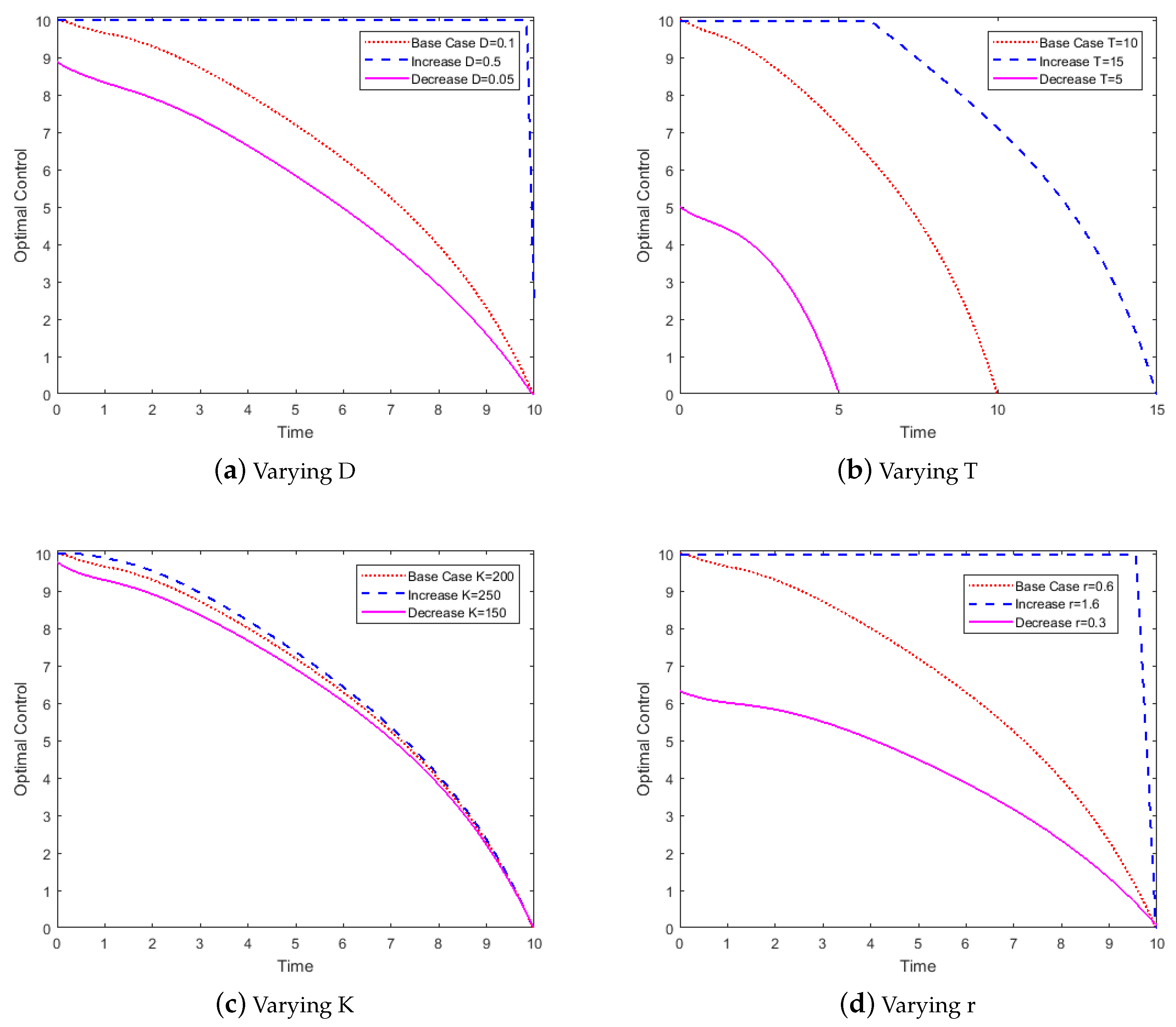
3.1. Cross-Sectional Area Is Constant

We begin these numerical simulations assuming our cross-sectional area, A, is constant. Later, we will vary it with respect to space and time. To illustrate the spread of a population in a river with control, we use the following Base Case parameters:

$$\begin{array}{cc}\hfill & T=10(\mathrm{final}\mathrm{time}),L=10(\mathrm{length}\mathrm{of}\mathrm{river}),\hfill \\ \hfill & r=0.6,K=200,D=0.1,A=20,ϵ=0.05,0\le Q\left(t\right)\le 10.\hfill \end{array}$$

(7)

Note that the downstream is represented by $x=L$. Figure 1 shows the initial condition and the weight function used in our simulations. In Figure 1a, we place the initial population downstream to see their movement upstream. In Figure 1b, we use a weight function that has values 100 upstream (at $x=0$) and nearly 0 upstream (at $x=10$). Recall that we are minimizing the objective functional, so this weight function helps push the population downstream.

We first illustrate how far the population moves upstream with no control, constant control, and optimal control in Figure 2. To generate this graph, we use a lower bound of 0.5 for the population, so, for each time, we find the lowest location x (more upstream) with $N(x,t)>0.5$ and record that river location. The constant control has the value of the upper bound of the optimal control. The population with no control moves further upstream than the population with constant control, which is to be expected. The population with no control moves from 8 to about $2.8$, which is about two-thirds upstream. The population with constant control starts at 8 and ends about $7.1$. Having a constant control at the upper bound ($Q=10$) resulted in the least movement upstream. With the optimal control, the population moves further upstream than the constant control case. Note that the optimal control is not at its upper bound for the whole time period due to costs in J. The objective functional balances keeping the population downstream with costs. The population in the optimal control case starts at 8 and ends around $5.5$.

Figure 3 shows the population plots for no control (Figure 3a) and for optimal control (Figure 3b). The population in the no control case spreads farther upstream than in the optimal control case. The population also grows larger in the no control case. In Figure 3c, the populations at the final time are plotted for the length of the river. The no control population is further upstream and is approaching the carrying capacity while the optimal control population only reached a value of about 140 at any given river location. The population size was decreased, and the population was kept more downstream in the optimal control case. Our objective functional value for the no control case is 239.57, while, for the optimal control case, is 40.12, which is an 83% improvement.

We varied parameters for the no control, constant control, and optimal control cases and show the changes in our objective functional J values. Starting with our Base Case parameter values in (7), we changed the values of D, T, r and K and investigated the resulting changes in J.

Table 1. Objective functional outputs for the cases tested where we changed the parameter values for D and T (given below). The base values are from the list (7). Constant control was run with $Q=10$.

	Base Case	$\mathit{D}=0.05$	$\mathit{D}=0.5$	$\mathit{T}=5$	$\mathit{T}=15$
No Control	239.52	111.96	5485.3	17.13	2373
Constant Control	56.63	53.72	316.89	28.39	84.87
Optimal Control	40.12	29.40	316.56	12.31	68.17

shows the J values for the Base Case along with cases with changes of D and T while

Table 2. Objective functional outputs for the cases tested where we changed parameter values for K and r (given below). The base values are from the list (7). Constant control was run with $Q=10$.

	Base Case	$\mathit{K}=150$	$\mathit{K}=250$	$\mathit{r}=0.3$	$\mathit{r}=1.6$
No Control	239.52	204.28	269.14	55.18	3837.3
Constant Control	56.63	56.16	56.97	52.44	176.67
Optimal Control	40.12	37.96	41.13	20.29	176.55

shows the variation of K and r. In all cases, the objective functional from the optimal control was smaller than the objective functional for the constant control and the no control cases, which is expected. In Figure 4, we plot the optimal controls for each of the parameters varied. Before changing any parameters for the Base Case, the optimal control is a 29% decrease in the objective functional from the constant control. This indicates that a time varying control can be significantly effective.

In Table 1, for the decrease in diffusion coefficient D, we see a 45% decrease in the objective functional from the constant control to the optimal control and a 74% decrease from the no control to optimal control. When we increase diffusion, there is almost no change in the J values for the constant control and optimal control. There is a 94% decrease from the objective functional value from the no control to the optimal control J value. Figure 4a shows the different optimal controls. When we increase the diffusion coefficient, the optimal control is at the upper bound for most of the time, which explains why the objective functional value was similar to the constant control one. Decreasing the diffusion creates a similar curve to the Base Case, but the optimal control values are slightly smaller. Returning to Table 1, decreasing the final time yields a 57% decrease in the objective functional from the constant control population to the optimal control population, and a 28% decrease from the no control to the optimal control. Meanwhile, increasing the final time gives a 20% decrease again from the constant control population to the optimal control population and a 97% decrease from no control to optimal control. In Figure 4b, increasing T causes the optimal control to be at the upper bound for about half the time, and to then steadily decrease to 0 at the final time. If we decrease T, the optimal control starts midway between the upper and lower bound and decreases down to 0 at the final time. The Base Case falls directly between these two cases.

Table 2 shows a 32% decrease in the objective functional from the constant control to the optimal control when we decrease the carrying capacity, K. Between the no control population and the optimal control population, there is a 81% decrease in the optimal control objective functional value. Increasing K yields a 28% decrease of J from the constant control to the optimal control, while a 85% decrease in J is seen from the no control case to the optimal control case. Figure 4c illustrates that increasing and decreasing K has little change in the optimal control values.

For decreasing the growth rate, r, there is a 61% reduction in the objective functional from the constant control population to the optimal control population. A decrease of 63% occurs in the objective functional values from the no control case to the optimal control case. When we increased r, there is virtually no change in the objective functional values between the constant control and the optimal control, but there was a 95% reduction in the J value from the no control population to the optimal control population. Figure 4d shows the optimal control at the upper bound for most of the time when we increase r. Decreasing r gives the optimal control initially at 6 and steadily decreases to 0 at the final time.

Since our objective functional is meant to represent minimizing the population at upstream and the cost of removing the invasive species, in most cases, using an optimal control would give at least a 20% decrease in $J\left(Q^{*}\right)$ from the constant control. In addition, the optimal control would give a smaller objective functional values $J\left(Q^{*}\right)$ than applying no control at all.

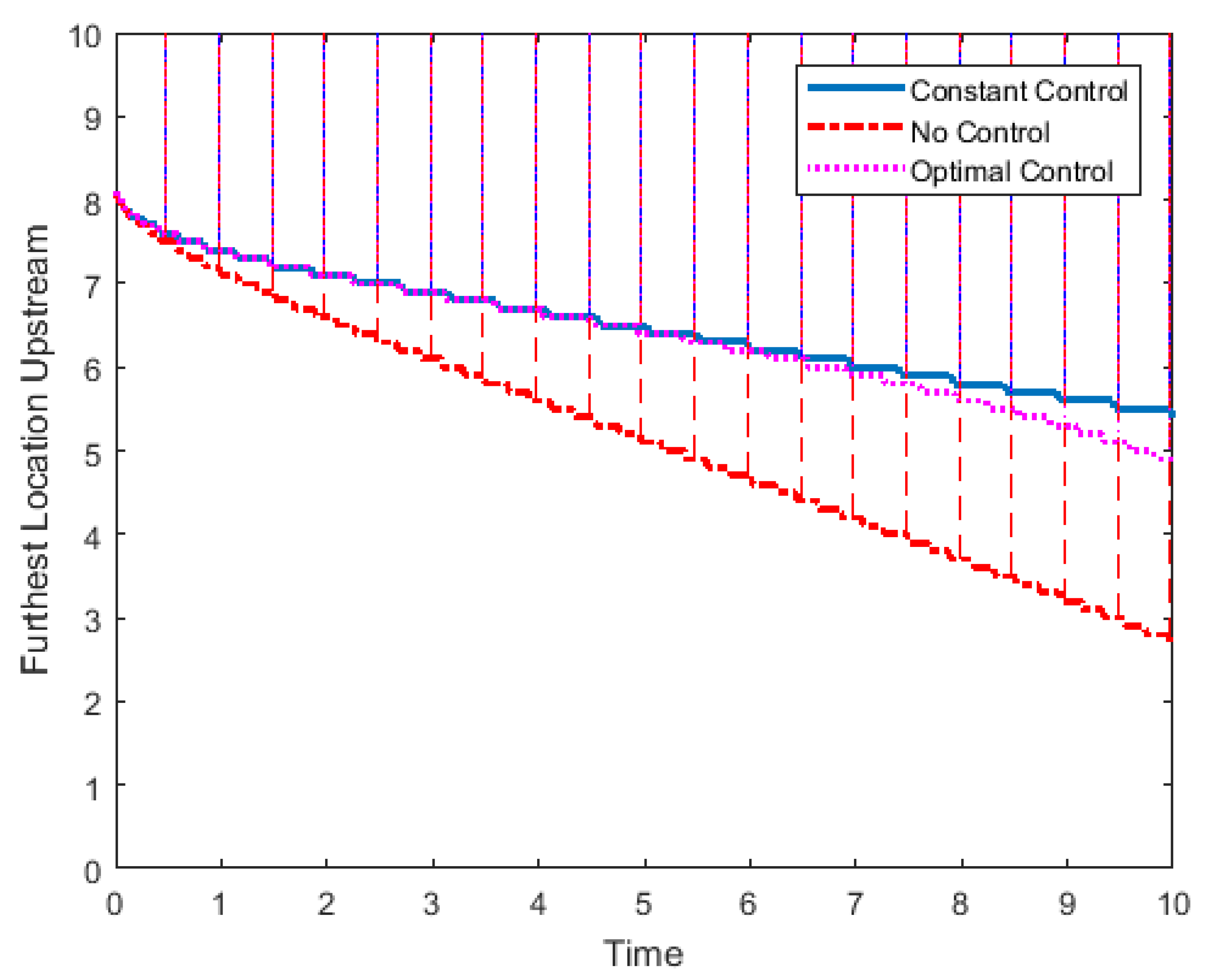
3.2. Cross-Sectional Area Is Not Constant

We now have the cross-sectional area dependent on space with a linear function,

$$A\left(x\right)=0.5x+25,$$

and ran all the same cases (varying D, T, K, and r) as for a constant cross-sectional area. The parameters are the same as before in the Base Case list (7). We do not show the specific graphs for this case, but we will compare the various location results later.

Finally, we let the cross-sectional area vary with time and space where

$$A(x,t)=\left(0.5x+25\right)+\left(0.2t\left(10-t\right)\right).$$

We chose a function so that the river was higher in the middle of the year. Again, the parameters are all the same as in the Base Case list (7). In Figure 5, the no control population starts at 8 and moves to 2.8 with an objective functional value of 238.66. The population with constant control moves from 8 to 5.5 with an objective functional value of 74.70. The population with the optimal control starts at 8 and ends at 4.9. The objective functional value for the optimal control is 66.55, which is again a 10.9% decrease from the constant control and a 72.1% decrease from the no control case. Figure 6 shows the population plots for the no control and optimal control cases, and, as expected, the population in the no control case is larger.

We compare the optimal control results for the three different cross-sectional area functions. We have that $25\le A\left(x\right)\le 35$ and $25\le A(x,t)\le 35$, while the constant $A=20$. In Figure 7, in the constant cross-sectional area case, the population moved upstream the least, at 5.5 at the furthest point. In addition, notice that $A\left(x\right)$ and $A(x,t)$ caused similar movement upstream. When the cross-sectional area is not constant, the species is able to move further upstream, possibly due to larger cross-sectional area. The objective functional values are 40.12 for constant A, 60.55 for $A\left(x\right)$, and 66.55 for $A(x,t)$. The J values increase as our cross-sectional areas become larger and more complex. This makes sense as the effort to keep the population downstream would become more difficult with the varying larger areas.

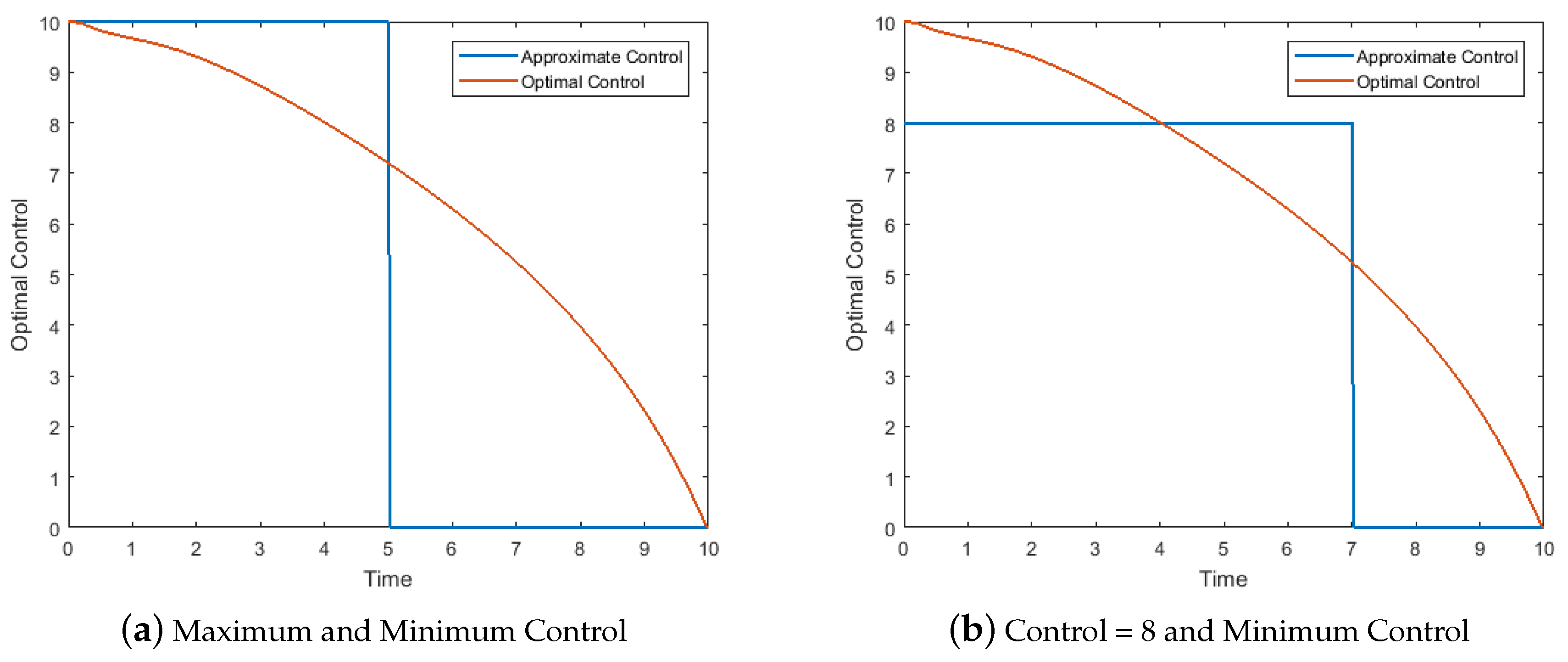
3.3. Approximate Controls

Optimal controls may change at every time step. However, changing river flow at every time step may be difficult, so we may use an optimal control to design an approximate control that is easier to implement. For example, using the optimal control as a guide, we design an approximate control where we set the control at a high value at the beginning time and a low value towards the end of our time period. In Figure 8a, we set the control, Q, to 10 for $t\le 5$ and then $Q=0$ for $t>5$, and plot this approximate control with the optimal control. For the approximate control, our objective functional value is 48.01, which is an increase from the 40.12 from the optimal control. In Figure 8b, another approximate control has $Q=8$ for $t\le 7$ and $Q=0$ for $t>7$. Here, our objective value is 42.49, which is again an increase compared to the Base Case value from the optimal control. This approximate control in Figure 8b is a good approximation since its corresponding J value is only 6% different from the optimal J.

We also changed the weight W in the objective function to be linear function and obtained quantitatively similar results. Changing the initial condition to be somewhat larger gives a larger objective functional values but with a similar optimal control.

4. Conclusions

To investigate how an invasive population moves upstream, we began with a PDE describing the movement of a species upstream, and then completed the needed analysis results for optimal control of this PDE using the flow rate as the control. We proved the differentiability of the control-to-state map as a directional derivative, which satisfies a linear sensitivity PDE. From the sensitivity PDE, we constructed our adjoint PDE that we used to characterize our optimal control. The control was chosen to keep the population downstream while minimizing the implementation cost.

To run numerical simulations to solve our optimality system, we used a finite difference method together with the forward-backward sweep method. In our simulations, we explored how changing the parameter values would affect the population’s location in the river and the J values for cases with no control, constant control, and optimal control while leaving our initial conditions the same for all cases and parameter changes. We first did this for a constant cross-sectional area of the river. As expected, we saw the optimal control populations were always an improvement in J on the no control populations and the constant control populations. The time varying control allowed for an immediate response to the changing population size. We also observed that varying the final time greatly changed the population’s location and size.

Changing the cross-sectional area to be dependent on space, and later on space and time, increased the J values from the constant cross-sectional area case with $A(x,t)$ being the largest. The non-constant A allowed the populations with constant and optimal controls to move further upstream than before (as seen in Figure 2, Figure 5, and Figure 7). The population probably moved farther upstream since there is more room for the species to move in the river for the $A\left(x\right)$ and $A(x,t)$ cases due to larger sizes of the cross-sections.

We investigated how our objective functional values changed if we implemented approximate controls that are easily implemented. We constructed an approximate control that gave a J value close to the optimal value.

Using optimal control theory can give strategies for controlling a flow rate to successfully manage a population in a river. Our future work will be to obtain some data for a particular invasive river species and apply these techniques. After approximating parameters and choosing appropriate cross-sectional area for a particular species in a river, we would explore how our optimal control strategy would affect the movements of the invasive population. We would also want to investigate more realistic cross-sectional area functions to better represent a river. Considering only allowing seasonal changes in controls would also be important for some situations.

References

1. Kolar, C.S.; Chapman, D.C.; Courtenay, W.R.; Housel, C.M.; Williams, J.D.; Jennings, D.P. Bigheaded Carps: A Biological Synopsis and Environmental Risk Assessment; American Fisheries Society: Bethesda, MD, USA, 2007. [Google Scholar]
2. Simberloff, D. Invasive Species: What Everyone Needs to Know; Oxford University Press: New York, NY, USA, 2013. [Google Scholar]
3. Lockwood, J.L.; Hoopes, M.F.; Marchetti, M.P. Invasion Ecology; Blackwell Publishing: Malden, MA, USA, 2007. [Google Scholar]
4. Jacobsen, J.; Jin, Y.; Lewis, M.A. Integrodifference models for persistence in temporally varying river environments. J. Math. Biol. 2015, 70, 549–590. [Google Scholar] [CrossRef] [PubMed]
5. Jin, Y.; Lewis, M.A. Seasonal influences on population spread and persistence in streams: critical domain size. SIAM J. Appl. Math. 2011, 71, 1241–1262. [Google Scholar] [CrossRef]
6. Jin, Y.; Lewis, M.A. Seasonal influences on population spread and persistence in streams: Spreading speeds. J. Math. Biol. 2012, 65, 403–439. [Google Scholar] [CrossRef]
7. Gagnon, K.; Peacock, S.J.; Jin, Y.; Lewis, M.A. Modelling the spread of the invasive alga Codium fragile driven by long-distance dispersal of buoyant propagules. Ecol. Model. 2015, 316, 111–121. [Google Scholar] [CrossRef]
8. Jin, Y.; Hilker, F.M.; Steffler, P.M.; Lewis, M.A. Seasonal Invasion Dynamics in a Spatially Heterogeneous River with Fluctuating Flows. Bull. Math. Biol. 2014, 76, 1522–1565. [Google Scholar] [CrossRef] [PubMed]
9. Clifford, N.J.; Harmar, O.P.; Harvey, G.; Petts, G.E. Physical habitat, eco-hydraulics and river design: A review and re-evaluation of some popular concepts and methods. Aquat. Conserv. Mar. Freshw. Ecosyst. 2006, 16, 389–408. [Google Scholar] [CrossRef]
10. Huang, Q.; Jin, Y.; Lewis, M.A. R0 analysis of a benthic-drift model for a stream population. SIAM J. Appl. Dyn. Syst. 2016, 15, 287–321. [Google Scholar] [CrossRef]
11. Jin, Y.; Lutscher, F.; Pei, Y. Meandering rivers: How important is lateral variability for species persistence? Bull. Math. Biol. 2017, 79, 2954–2985. [Google Scholar] [CrossRef] [PubMed]
12. Poff, N.L.; Zimmerman, J.K. Ecological responses to altered flow regimes: A literature review to inform the science and management of environmental flows. Freshw. Biol. 2010, 55, 194–205. [Google Scholar] [CrossRef]
13. De Silva, K.R.; Phan, T.V.; Lenhart, S. Advection control in parabolic PDE systems for competitive populations. Discret. Contin. Dyn. Syst. Ser. B 2017, 22, 1049–1072. [Google Scholar] [CrossRef] [Green Version]
14. Kelly, M.; Xing, Y.; Lenhart, S. Optimal fish harvesting for a population modeled by a nonlinear parabolic partial differential equation. Nat. Resour. Model. J. 2016, 29, 36–70. [Google Scholar] [CrossRef]
15. Simon, J. Compact sets in the Lp(0,t:b). Ann. Mat. Pura Appl. 1987, 146, 65–96. [Google Scholar] [CrossRef]
16. Lions, J.L. Equations Différentielles Opérationnelles et Problèmes aux Limites; Springer: Berlin, Germany, 1961. [Google Scholar]
17. Friedman, A. Foundations of Modern Analysis; Dover Publications: New York, NY, USA, 1970. [Google Scholar]
18. Evans, L. Partial Differential Equations; American Mathematical Society: Providence, RI, USA, 2010. [Google Scholar]
19. Lenhart, S. Optimal Control of a Convective Diffusive Fluid Problem. Math. Models Methods Appl. Sci. 1995, 5, 225–237. [Google Scholar] [CrossRef]
20. Ladyzenskaja, O.A.; Solonnikov, V.A.; Ural’ceva, N.N. Linear and Quasi-Linear Equations of Parabolic Type; American Mathematical Society: Providence, RI, USA, 1968. [Google Scholar]
21. Li, X.; Yong, J. Optimal Control for Infinite Dimensional Systems; Birkhauser: Boston, MA, USA, 1995. [Google Scholar]
22. Hackbush, W. A numerical method for solving parabolic equations with opposite orientations. Computing 1978, 20, 229–240. [Google Scholar] [CrossRef]
23. Lenhart, S.; Workman, J.T. Optimal Control Applied to Biological Models; Chapman and Hall/CRC: Boca Raton, FL, USA, 2007. [Google Scholar]
24. Iserles, A. A First, Course in the Numerical Analysis of Differential Equations; Cambridge University Press: New York, NY, USA, 2008. [Google Scholar]
Figure 1. (a) The initial condition for the population; (b) the weight function in the objective functional.
Mathematics 07 00975 g001
Figure 2. Location of the population in the river for the no control case (red), for the constant control case with Q = 10 (blue), and the optimal control case (magenta) over the time, with parameter values fromtje Base Case list (7).
Mathematics 07 00975 g002
Figure 3. Population plots for (a) no control case and (b) optimal control case; (c) population plots in x at the final time for both cases. The parameter values are from the Base Case list (7).
Mathematics 07 00975 g003
Figure 4. The optimal control plots for varying of the parameters D, T, K, and r. The base parameter values are from the list (7).
Mathematics 07 00975 g004
Figure 5. Location of the population in the river for the no control case (red), for the constant control case with Q = 10 (blue), and the optimal control case (magenta) over the time with the cross-sectional area is dependent on space and time, A ( x , t ) = 0.5 x + 25 + 0.2 t 10 t . The parameter values are T = 10 , L = 10 , r = 0.6 , K = 200 , D = 0.1 , and 0 Q ( t ) 10 .
Mathematics 07 00975 g005
Figure 6. The population plots for the (a) no control case and (b) the optimal control case with the cross-sectional area is dependent on space and time, A ( x , t ) = 0.5 x + 25 + 0.2 t 10 t . The parameter values are from the Base Case list (7).
Mathematics 07 00975 g006
Figure 7. Location of the population in the river for the optimal control where the different cross-sectional area values are: constant A = 20 (blue), A ( x ) = 0.5 x + 25 (magenta), and A ( x , t ) = 0.5 x + 25 + 0.2 t 10 t (red). The parameter values are from the Base Case list (7).
Mathematics 07 00975 g007
Figure 8. Control plots for both the optimal control case and two constant case. (a) the two constant control case where Q = 10 for t 5 and Q = 0 for t > 5 , and (b) the two constant control case where Q = 8 for t 7 and Q = 0 for t > 7 . The parameter values are from the Base Case list (7).
Mathematics 07 00975 g008