Article

Approximate Solutions of Time Fractional Diffusion Wave Models

1
Institute of Numerical Sciences, Kohat University of Science and Technology, Kohat 26000, KP, Pakistan
2
Faculty of Engineering Sciences, GIK Institute, Topi 23640, KP, Pakistan
3
Theoretical and Computational Science (TaCS) Center Department of Mathematics, Faculty of Science, King Mongkuts University of Technology Thonburi (KMUTT), 126 Pracha Uthit Rd., Bang Mod, Thung Khru, Bangkok 10140, Thailand
4
KMUTT-Fixed Point Research Laboratory, Room SCL 802 Fixed Point Laboratory, Science Laboratory Building, Department of Mathematics, Faculty of Science, King Mongkut’s University of Technology Thonburi (KMUTT), 126 Pracha-Uthit Road, Bang Mod, Thrung Khru, Bangkok 10140, Thailand
5
Department of Medical Research, China Medical University Hospital, China Medical University, Taichung 40402, Taiwan
*
Author to whom correspondence should be addressed.
Mathematics 2019, 7(10), 923; https://doi.org/10.3390/math7100923
Submission received: 11 July 2019 / Revised: 14 August 2019 / Accepted: 27 August 2019 / Published: 3 October 2019

Abstract

:
In this paper, a wavelet based collocation method is formulated for an approximate solution of (1 + 1)- and (1 + 2)-dimensional time fractional diffusion wave equations. The main objective of this study is to combine the finite difference method with Haar wavelets. One and two dimensional Haar wavelets are used for the discretization of a spatial operator while time fractional derivative is approximated using second order finite difference and quadrature rule. The scheme has an excellent feature that converts a time fractional partial differential equation to a system of algebraic equations which can be solved easily. The suggested technique is applied to solve some test problems. The obtained results have been compared with existing results in the literature. Also, the accuracy of the scheme has been checked by computing L 2 and L error norms. Computations validate that the proposed method produces good results, which are comparable with exact solutions and those presented before.

1. Introduction

The theory of fractional calculus is an ancient topic that has many applications. However, practical work in this direction has been recently started (see References [1,2,3]). Most of the physical phenomena in chemistry, physics, engineering and other fields of science can be modeled using parameters of fractional calculus [4,5], means fractional derivative and integral operators. Amongst these are electrolyte polarization [6], viscoelastic systems [7], dielectric polarization [8] and so forth. Fractional models in different circumstances lead towards more accurate behaviour than those of integer order models.
The time fractional diffusion wave equation (TFDWE) is such an important model which has extensive uses. The TFDWE is actually a wave equation [9] with a fractional time derivative which describes universal acoustic, electromagnetic and mechanical responses [10,11] with an enhanced method. Over the past few decades, extensive attention has been paid to the closed form solution of time fractional diffusion wave equations (TFDWEs) and is still an open area of research. The closed form solution of such problems is not an easy job and needs herculean efforts. Owing to the fact several authors proposed numerical methods for the solution of fractional models, Tadjeran et al. [12] used second order accurate approximation for fractional diffusion equations. Zhuang et al. [13] applied an implicit numerical method for the anomalous sub-diffusion equation. Yuste and Acedo [14] studied fractional diffusion equations via an explicit finite difference method. Chen et al. [15] proposed the Fourier method for fractional diffusion equations. Hosseini et al. [16] solved the fractional telegraph equation with the help of radial basis functions. Zhou and Xu [17] applied the Chebyshev wavelets collocation method for the solution of time fractional diffusion wave equations. Bhrawya [18] used the spectral Tau algorithm based on the Jacobi operational matrix for the numerical solution of time fractional diffusion-wave equations. Yaseen et al. [19] solved fractional diffusion wave equations with reaction terms using finite differences and a trigonometric B-splines technique. Khader [20] and his co-author applied the finite difference method coupled with the Hermite formula for solutions of fractional diffusion wave equations. Kanwal et al. [21] implemented two-dimensional Genocchi Polynomials combined with the Ritz-Galerkin Method for solutions of fractional diffusion wave and Klein-Gordon equations. Datsko et al. [22] studied time-fractional diffusion-wave equation with mass absorption in a sphere under harmonic impact.
Recently, numerical methods using wavelets have been given more emphasis because of their simple applicability. These methods also have some other interesting properties such as the ability to detect singularities and express the function in different resolution levels, which improves the accuracy. Amongst different classes of wavelets, Haar wavelets deserve special consideration. Haar wavelets consist of piece wise constant functions. The integration of these wavelets in different times is one of the best features. Also, Haar wavelets have orthogonality and normalization properties with compact support. For more discussion on Haar wavelets one can see References [23,24].
In the present study, we propose a hybrid numerical scheme, based on Haar wavelets and finite differences, to solve (1 + 1)- and (1 + 2)-dimensional TFDWEs. The stability of the proposed method is discussed with the matrix method which is an essential part of the manuscript. The models which will be under consideration are characterized in the following types:
  • (1 + 1)-Dimensional Equation:
    c D t δ w ( x , t ) = w t ( x , t ) + w x x ( x , t ) + A ( x , t ) , x Ω , t [ 0 , T ] , 1 < δ 2 ,
    w ( x , 0 ) = f ( x ) , w t ( x , 0 ) = g ( x ) x Ω ˜ = Ω Ω , w ( x , t ) = α ( t ) , x Ω t [ 0 , T ] .
  • (1 + 2)-Dimensional Equation:
    c D t δ w ( x , y , t ) = Δ w ( x , y , t ) + B ( x , y , t ) , ( x , y ) Φ , t [ 0 , T ] , 1 < δ 2 ,
    w ( x , y , 0 ) = χ ( x , y ) , w t ( x , y , 0 ) = κ ( x , y ) , ( x , y ) Φ ˜ = Φ Φ , w ( x , y , t ) = χ 1 ( x , y , t ) , ( x , y ) Φ , t [ 0 , T ] .
In Equations (1)–(4), Δ is two-dimensional Laplacian; A , B , f , g , α , χ , κ , χ 1 are known functions and w is unknown function. Equations (2) and (4) are the corresponding initial and boundary conditions. The symbols, Ω and Ω , Φ and Φ represent the domain and boundary of the domain respectively for (1 + 1)- and (1 + 2)-dimensional problems. Also c D t δ w denotes the time fractional derivative of w with respect to t in the Caputo sense which is given by
c D t δ w = 1 Γ 2 δ 0 t w ζ ζ ( x , ζ ) t ζ δ 1 d ζ , 1 < δ < 2 , 2 w ( x , t ) t 2 , δ = 2 .

2. Ground Work

In this section, some basic definitions of fractional calculus and Haar wavelets are presented, which will be required for the demonstration of our results. For a basic definition of Haar wavelets and its integrals we refer to Reference [23]. Let us consider x [ a , b ] where a and b are the limits of the interval. Next, the interval is subdivided into 2 M intervals where M = 2 J and J denote the maximal level of resolution. Further, the two parameters j = 0 , . , J and k = 0 , . , 2 j 1 are introduced. These parameters show the integer decomposition of wavelet number i = m + k + 1 , where m = 2 j . The first and ith wavelets are defined as follows:
H 1 ( x ) = 1 , x a , b 0 , otherwise .
H i ( x ) = 1 , x ξ 1 ( i ) , ξ 2 ( i ) 1 , x ξ 2 ( i ) , ξ 3 ( i ) 0 , otherwise ,
where
ξ 1 ( i ) = a + 2 k ν δ x , ξ 2 ( i ) = a + ( 2 k + 1 ) ν δ x , ξ 3 ( i ) = a + 2 ( k + 1 ) ν δ x , ν = M m , δ x = b a 2 M .
To solve n t h order time fractional PDEs the following repeated integrals are needed:
P i , β ( x ) = a x a x a x H i ( z ) d z β = 1 β 1 ! a x x z β 1 H i ( z ) d z ,
where
β = 1 , 2 , n , i = 1 , 2 , 2 M .
Keeping in view Equations (6) and (7) the close form expressions of these integrals are given by
P 1 , β ( x ) = x a β β ! .
P i , β ( x ) = 0 , x < ξ 1 ( x ) 1 β ! x ξ 1 ( i ) β x ξ 1 ( i ) , ξ 2 ( i ) 1 β ! ( x ξ 1 ( i ) ) β 2 ( ( x ξ 2 ( i ) ) β x [ ξ 2 ( i ) , ξ 3 ( i ) ) 1 β ! ( x ξ 1 ( i ) ) β 2 ( ( x ξ 2 ( i ) ) β + ( x ξ 3 ( i ) ) β x ξ 3 ( i ) .

3. Description of the Method

This section is devoted to discussing the scheme for Equations (1) and (3) separately. In both cases, the fractional order time derivative has been approximated by the quadrature formula [16]
c D t δ w ( x , t j + 1 ) = 1 Γ 2 δ 0 t j + 1 w ( 2 ) ( x , ζ ) t j + 1 ζ 1 δ d ζ = 1 Γ 2 δ k = 0 j t j t j + 1 w k + 1 2 w k + w k 1 τ 2 t j + 1 ζ 1 δ d ζ = 1 Γ 2 δ k = 0 j w k + 1 2 w k + w k 1 τ 2 t j t j + 1 ( j + 1 ) τ ζ 1 δ d ζ = 1 Γ 2 δ k = 0 j w k + 1 2 w k + w k 1 τ 2 ( j k + 1 ) 2 δ ( j k ) 2 δ ( 2 δ ) ( τ δ 2 ) = τ δ Γ 3 δ k = 0 j w j k + 1 2 w j k + w j k 1 k + 1 2 δ k 2 δ = A δ w j + 1 2 w j + w j 1 + A δ k = 1 j w j k + 1 2 w j k + w j k 1 B ( k ) ,
where A δ = τ δ Γ 3 δ , τ is time step size and B ( k ) = k + 1 2 δ k 2 δ .
  • Case i:
Using Equation (11) and θ weighted scheme ( 0 θ 1 ) in Equation (1), we obtain
A δ w j + 1 2 w j + w j 1 + A δ k = 1 j w j k + 1 2 w j k + w j k 1 B ( k ) + 1 τ w j + 1 w j = θ w x x j + 1 + ( 1 θ ) w x x j + A ( x , t j + 1 ) .
After simplification, the above equation transforms to
( τ A δ + 1 ) w j + 1 τ θ w x x j + 1 = 2 τ A δ w j τ A δ w j 1 τ A δ k = 1 j w j k + 1 2 w j k + w j k 1 B ( k ) + w j + τ ( 1 θ ) w x x j + τ A ( x , t j + 1 ) .
In our analysis we take θ = 1 / 2 . Now approximating the highest order derivative by a truncated Haar wavelets series as:
w x x j + 1 ( x ) = i = 1 2 M a i j + 1 H i ( x ) .
Integrating Equation (14) from 0 to x
w x j + 1 ( x ) = i = 1 2 M a i j + 1 P i , 1 ( x ) + w x j + 1 ( 0 ) .
Integrating Equation (15) from 0 to 1, we get
w x j + 1 ( 0 ) = w j + 1 ( 1 ) w j + 1 ( 0 ) i = 1 2 M a i j + 1 P i , 2 ( 1 ) .
Substituting Equation (16) in Equation (15), the resultant equation reduces to
w x j + 1 ( x ) = i = 1 2 M a i j + 1 P i , 1 ( x ) P i , 2 ( 1 ) + w j + 1 ( 1 ) w j + 1 ( 0 ) .
Integration of Equation (17) from 0 to x yields
w j + 1 ( x ) = i = 1 2 M a i j + 1 P i , 2 ( x ) x P i , 2 ( 1 ) + x w j + 1 ( 1 ) w j + 1 ( 0 ) + w j + 1 ( 0 ) .
Substituting values from Equations (14), (17) and (18) in Equation (13) and using collocation points x m = m 0.5 2 M , m = 1 , 2 , 2 M , leads to the following system of algebraic equation
i = 1 2 M a i j + 1 τ A δ + 1 { P i , 2 ( x ) x P i , 2 ( 1 ) } τ θ H i ( x ) x = x m = R ( m ) ,
where
R ( m ) = 2 τ A δ w j τ A δ w j 1 τ A δ k = 1 j w j k + 1 2 w j k + w j k 1 B ( k ) + w j + τ ( 1 θ ) w x x j + τ A ( x m , t j + 1 ) τ A δ + 1 x m w j + 1 ( 1 ) w j + 1 ( 0 ) + w j + 1 ( 0 ) .
Equation (19) contains 2 M equations. The unknown wavelet coefficients can be computed from this system. After determination of these unknown constants, the required solution at each time can be calculated from Equation (18).
  • Case ii:
Following a similar approach, as discussed earlier, Equation (3) gives
A δ w j + 1 θ w x x j + 1 + w y y j + 1 = ( 1 θ ) w x x j + w y y j + B ( x , y , t j + 1 ) + 2 A δ w j A δ w j 1 A δ k = 1 j w j k + 1 2 w j k + w j k 1 B ( k ) .
Now we approximate w x x y y j + 1 ( x , y ) with a two dimensional truncated Haar wavelets series as:
w x x y y j + 1 ( x , y ) = i = 1 2 M l = 1 2 M a i , l j + 1 H i ( x ) H i ( y ) ,
where a i , l j + 1 are unknowns to be determined. Integration of Equation (21) w.r.t. to y, between 0 and y, gives
w x x y j + 1 ( x , y ) = i = 1 2 M l = 1 2 M a i , l j + 1 H i ( x ) P l , 1 ( y ) + w x x y j + 1 ( x , 0 ) .
Integrating Equation (22) w.r.t y from 0 to 1, the unknown term w x x y j + 1 ( x , 0 ) is given by
w x x y j + 1 ( x , 0 ) = w x x j + 1 ( x , 1 ) w x x j + 1 ( x , 0 ) i = 1 2 M l = 1 2 M a i , l j + 1 H i ( x ) P l , 2 ( 1 ) .
Substituting Equation (23) in Equation (22), the obtained result is
w x x y j + 1 ( x , y ) = i = 1 2 M l = 1 2 M a i , l j + 1 H i ( x ) P l , 1 ( y ) P l , 2 ( 1 ) + w x x j + 1 ( x , 1 ) w x x j + 1 ( x , 0 ) .
Integrating Equation (24) from 0 to y, we get
w x x j + 1 ( x , y ) = i = 1 2 M l = 1 2 M a i , l j + 1 H i ( x ) P l , 2 ( y ) y P l , 2 ( 1 ) + y w x x j + 1 ( x , 1 ) + ( 1 y ) w x x j + 1 ( x , 0 ) .
Repeating the same procedure one can easily derive the subsequent expressions
w y y j + 1 ( x , y ) = i = 1 2 M l = 1 2 M a i , l j + 1 P i , 2 ( x ) x P i , 2 ( 1 ) H l ( y ) + x w y y j + 1 ( 1 , y ) + 1 x w y y j + 1 ( 0 , y ) .
w x j + 1 ( x , y ) = i = 1 2 M l = 1 2 M a i , l j + 1 P i , 1 ( x ) P i , 2 ( 1 ) P l , 2 ( y ) y P l , 2 ( 1 ) + y w x j + 1 ( x , 1 ) + ( 1 y ) w x j + 1 ( x , 0 ) + w j + 1 ( 1 , y ) w j + 1 ( 0 , y ) y w j + 1 ( 1 , 1 ) + y w j + 1 ( 0 , 1 ) + ( y 1 ) w j + 1 ( 1 , 0 ) + ( 1 y ) w j + 1 ( 0 , 0 ) .
w y j + 1 ( x , y ) = i = 1 2 M l = 1 2 M a i , l j + 1 P i , 2 ( x ) x P i , 2 ( 1 ) P l , 1 ( y ) P l , 2 ( 1 ) + x w y j + 1 ( 1 , y ) + ( 1 x ) w y j + 1 ( 0 , y ) + w j + 1 ( x , 1 ) w j + 1 ( x , 0 ) x w j ( 1 , 1 ) + x w j + 1 ( 1 , 0 ) + ( x 1 ) w j + 1 ( 0 , 1 ) + ( 1 x ) w j + 1 ( 0 , 0 ) .
w j + 1 ( x , y ) = i = 1 2 M l = 1 2 M a i , l j + 1 P i , 2 ( x ) x P i , 2 ( 1 ) P l , 2 ( y ) y P l , 2 ( 1 ) + y w j + 1 ( x , 1 ) y w j + 1 ( 0 , 1 ) + ( 1 y ) w j + 1 ( x , 0 ) w j + 1 ( 0 , 0 ) + x w j + 1 ( 1 , y ) x w j + 1 ( 0 , y ) x y w j + 1 ( 1 , 1 ) w j + 1 ( 0 , 1 ) + x y 1 w j + 1 ( 1 , 0 ) + x ( 1 y ) w j + 1 ( 0 , 0 ) + w j + 1 ( 0 , y ) .
Substitution of Equations (25), (26) and (29) in Equation (20) and using the collocation points, x m = m 0.5 2 M , y n = n 0.5 2 M , m , n = 1 , 2 , 2 M , produces the following system of equations
i = 1 2 M l = 1 2 M a i , l j + 1 A δ D ( i , l , m , n ) θ E ( i , l , m , n ) θ F ( i , l , m , n ) = L ( m , n ) + M ( m , n ) ,
where
D ( i , l , m , n ) = P i , 2 ( x m ) x m P i , 2 ( 1 ) P l , 2 ( y n ) y n P l , 2 ( 1 ) , E ( i , l , m , n ) = H i ( x m ) P l , 2 ( y n ) y n P l , 2 ( 1 ) , F ( i , l , m , n ) = P i , 2 ( x m ) x m P i , 2 ( 1 ) H l ( y n ) , L ( m , n ) = ( 1 θ ) w x x j + w y y j , + B ( x m , y n , t j + 1 ) + 2 A δ w j A δ w j 1 A δ k = 1 j w j k + 1 2 w j k + w j k 1 B ( k ) , M ( m , n ) = A δ [ y n w x j + 1 ( x m , 1 ) y n w j + 1 ( 0 , 1 ) + ( 1 y n ) w j + 1 ( x m , 0 ) w j + 1 ( 0 , 0 ) + x m w j + 1 ( 1 , y n ) x m w j + 1 ( 0 , y n ) x m y n w j + 1 ( 1 , 1 ) w j + 1 ( 0 , 1 ) + x m y n 1 w j + 1 ( 1 , 0 ) + x m ( 1 y n ) w j + 1 ( 0 , 0 ) + w j + 1 ( 0 , y n ) ] + θ [ y n w x x j + 1 ( x m , 1 ) + ( 1 y n ) w x x j + 1 ( x m , 0 ) + x m w y y j + 1 ( 1 , y n ) + 1 x m w y y j + 1 ( 0 , y n ) ] .
Equation (30) represents 2 M × 2 M equations in so many unknowns which can be solved easily. After calculation of these unknowns, an approximate solution can be obtained from Equation (29).

4. Stability Analysis

Here we present the stability analysis of the proposed scheme for (1 + 2)-dimensional problems; a similar result can be proved for (1 + 1)-dimensional problems. In matrix form Equations (25), (26) and (29) can be written as
w x x j + 1 = U α j + 1 + U ˜ j + 1 ,
w y y j + 1 = V α j + 1 + V ˜ j + 1 ,
w j + 1 = Z α j + 1 + Z ˜ j + 1 ,
where α j + 1 = α j + 1 ( i , l ) , U , V , Z and U ˜ j + 1 , V ˜ j + 1 , Z ˜ j + 1 are interpolation matrices of w x x j + 1 , w y y j + 1 , w j + 1 at collocation points and boundary terms, respectively. Now using Equations (31), (32) and (33) in Equation (20), we get
A δ Z θ U + V α j + 1 = 2 A δ Z + ( 1 θ ) U + V α j + G j + 1 ,
where G j + 1 = A δ Z ˜ j + 1 + θ U ˜ j + 1 + V ˜ j + 1 + 2 A δ Z j ˜ + ( 1 θ ) ( U j ˜ + V j ˜ ) + B j + 1 A δ w j 1 A δ k = 1 j w j k + 1 2 w j k + w j k 1 B ( k ) .
Now From Equation (34) one can write
α j + 1 = C 1 T α j + C 1 G j + 1 ,
where C = A δ Z θ U + V , T = 2 A δ Z + ( 1 θ ) U + V . Putting Equation (35) in Equation (33) we get
w j + 1 = Z C 1 T α j + Z C 1 G j + 1 + Z ˜ j + 1 .
Using Equation (33) in Equation (36) we have
w j + 1 = Z C 1 T Z 1 w j Z C 1 T Z 1 Z ˜ j + Z C 1 G j + 1 + Z ˜ j + 1 .
The above equation shows a recurrence relation of a full discretization scheme which allow us refinement in time. If w ˜ j + 1 is numerical solution then
w ˜ j + 1 = Z C 1 T Z 1 w j ˜ Z C 1 T C 1 Z ˜ j + Z C 1 G j + 1 + Z ˜ j + 1 .
Let e j + 1 = w j + 1 w ˜ j + 1 be the error at ( j + 1 ) t h time level. Subtracting Equation (37) from Equation (38) then
e j + 1 = Λ e j ,
where Λ = Z C 1 T Z 1 is the amplification matrix. According to Lax-Richtmyer criterion, the scheme will be stable if Λ 1 . It has been verified computationally that Λ 1 . For J = 1 the spectral radius is 0.01025 which lies in the stability domain.

5. Convergence Analysis

The convergence analysis of scheme (18) and (29) is similar to the following theorems, therefore the proofs are omitted.
Lemma 1
(see [24]). If w ( x ) L 2 ( R ) with | w ( x ) | ρ , for all x ( 0 , 1 ) , ρ > 0 and w ( x ) = i = 0 a i H i ( x ) then a i ρ 2 j + 1 .
Lemma 2
(see [25]). If f ( x , y ) satisfies a Lipschitz condition on [ 0 , 1 ] × [ 0 , 1 ] , that is, there exists a positive L such that for all ( x 1 , y ) , ( x 2 , y ) [ 0 , 1 ] × [ 0 , 1 ] we have f ( x 1 , y ) f ( x 2 , y ) L x 1 x 2 then
a i , l 2 L 2 2 4 j + 4 m 2
Theorem 1.
If w ( x ) and w 2 M ( x ) are the exact and approximate solution of Equation (1), then the error norm E J at J t h resolution level is
E J 4 ρ 3 1 2 J + 1 2 .
Proof. 
See [26]. ☐
Theorem 2.
Assume w ( x , y ) and w 2 M ( x , y ) be the exact and approximate solution of Equation (3), then
E J L 4 255 1 2 4 J .
Proof. 
See [27]. ☐

6. Illustrative Test Problems

In this part, we chose some test problem to confirm the reliability and efficiency of the present scheme. For validation of our results L and L 2 error norm are figured out which are defined as follows:
L 2 = i = 1 2 M w e x t w a p p 2 , L = max 1 i 2 M | w e x t w a p p | ,
where w a p p and w e x t are respectively approximate and exact solutions.
  • Problem 5.1
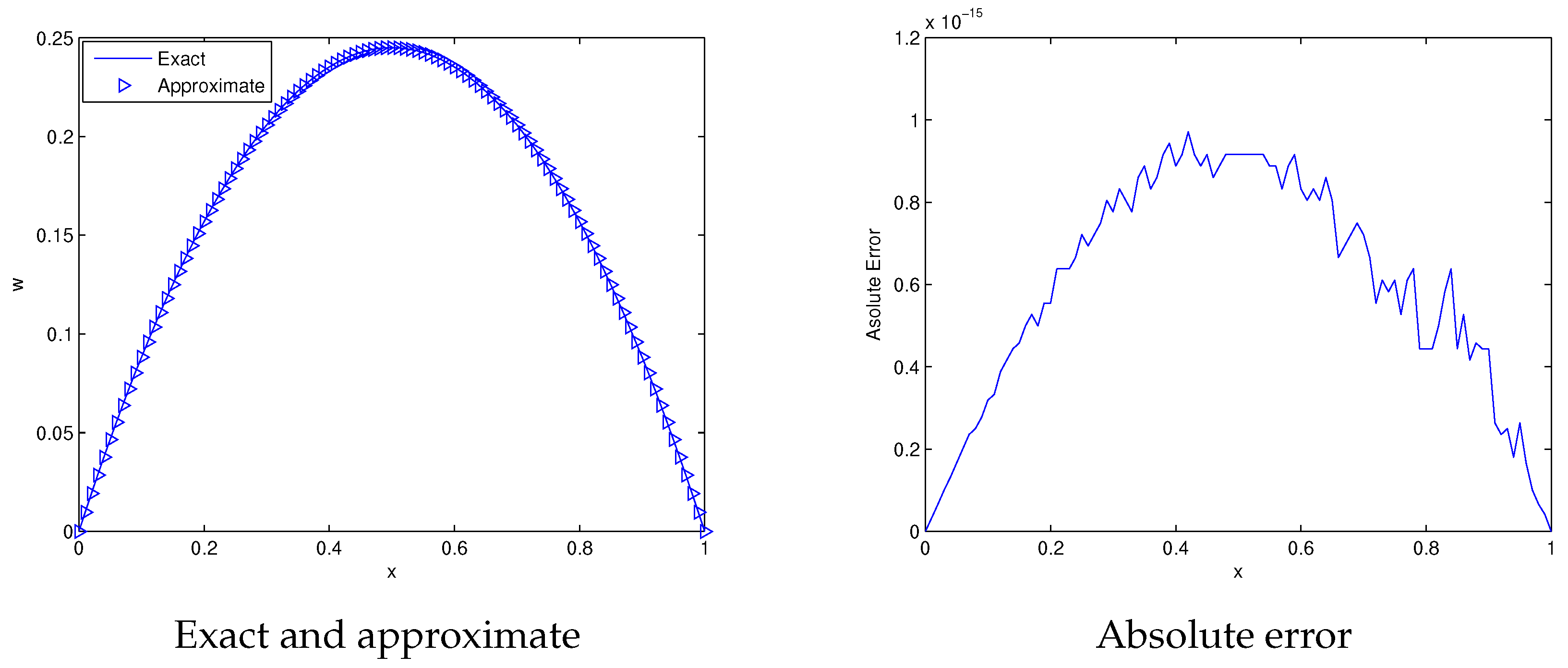
Let us take the following (1 + 1)-dimensional TFDWE with damping
c D t δ w ( x , t ) = w t ( x , t ) + w x x ( x , t ) + A ( x , t ) , x [ 0 , 1 ] , t [ 0 , 1 ] , 1 < δ 2 ,
with A ( x , t ) = 2 x ( 1 x ) t 2 δ Γ ( 3 δ ) + 2 t x ( 1 x ) + 2 t 2 . Initial and boundary conditions are derived from the exact solution w ( x , t ) = t 2 x ( 1 x ) . This problem has been solved for parameters J = 4 , t = 0.01 , 0.1 , 1 , δ = 1.1 , 1.3 , 1.5 , 1.7 , 1.9 . The obtained error norms are shown in Table 1. From table it is obvious that results of the present scheme match well with exact solution. Also in Table 2 it has been observed that accuracy increases with increasing resolution level which shows the convergence in the spatial direction. In the same table, the results have been matched with existing results in the literature which clarify that computed solutions are in good agreement with the work of Chen et al. [28]. Table 3 shows convergence in time for fixed d x = 1 / 32 . The convergence rate of the proposed scheme has been addressed in Table 4. the graphical solution and error plot are given in Figure 1. From this Figure it is clear that approximate solutions are matchable with exact.
  • Problem 5.2:
Consider the following TFDWE with damping
c D t δ w ( x , t ) = w t ( x , t ) + w x x ( x , t ) + A ( x , t ) , x [ 0 , 1 ] , t [ 0 , 1 ] , 1 < δ 2 ,
coupled with initial and boundary conditions
w ( x , 0 ) = 0 , w t ( x , 0 ) = 0 x ( 0 , 1 ) w ( 0 , t ) = t 3 , w ( 1 , t ) = e t 3 , t [ 0 , 1 ] .
The exact solution and source term are given by w ( x , t ) = e x t 3 and A ( x , t ) = 6 t 3 δ e x Γ ( 4 δ ) + 3 t 2 e x t 3 e x . In Table 5 the obtained error norms are shown for parameters t = 0.01 , 0.1 , δ = 1.1 , 1.3 , 1.5 , 1.7 , 1.9 , J = 4 . Table 5 shows that exact and approximate solutions agree with each other. The solution profile and absolute error are displayed Figure 2. From the Figure, the coincidence of both solutions are visible.
  • Problem 5.3:
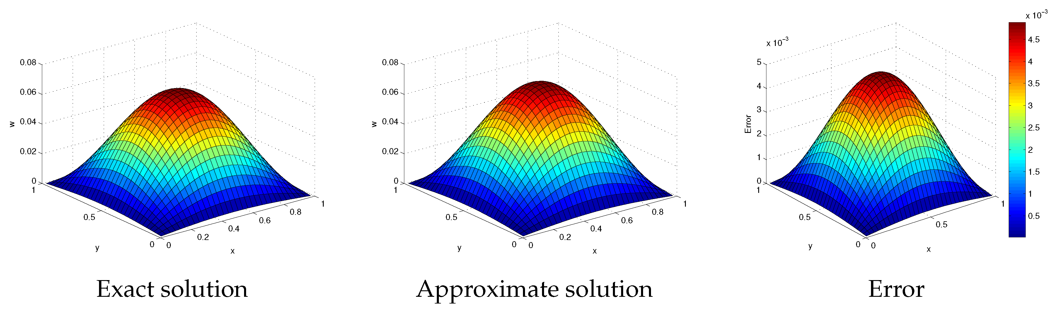
Now we consider (1+2)-dimensional TFDWE [29]
c D t δ w ( x , y , t ) = Δ w ( x , y , t ) + B ( x , y , t ) , ( x , y ) [ 0 , 1 ] × [ 0 , 1 ] , t [ 0 , 1 ] , 1 < δ 2 ,
with exact solution w ( x , y , t ) = s i n ( π x ) s i n ( π y ) t δ + 3 , and source term
B ( x , y , t ) = s i n ( π x ) s i n ( π y ) Γ ( δ + 3 ) t 2 2 2 t δ + 2 .
We solved this problem for resolution level J = 4 and the obtained results are recorded in Table 6 for different values of time and τ . From Table 6 it is clear that the proposed scheme works well for the solution of two dimensional problems. Table 7 shows the comparison of the computed results with the previous work of Zhang [29]. One can see that our results are matchable with existing results. The same table presents convergence in time for ( 1 + 2 ) -dimensional problems. The graphical solution and absolute error of the problem are shown in Figure 3. It is obvious from Figure 3 that the exact and approximate solutions have strong agreement.
  • Problem 5.4:
Consider the following TFDWE with reaction term [19]
c D t δ w ( x , t ) + w ( x , t ) = w x x ( x , t ) + A ( x , t ) , x [ 0 , 1 ] , t [ 0 , 1 ] , 1 < δ 2 ,
coupled with initial and boundary conditions
w ( x , 0 ) = 0 , w t ( x , 0 ) = 0 x ( 0 , 1 ) w ( 0 , t ) = o , w ( 1 , t ) = 0 , t [ 0 , 1 ] ,
where the forcing terms are A ( x , t ) = 2 t 2 δ x ( 1 x ) Γ ( 3 δ ) + t 2 x ( 1 x ) 2 t 2 . This problem has been solved with the help of the proposed scheme. In Table 8 we presented the solutions at different points. Also the obtained results have been compared with the work presented in Reference [19]. It is clear from table that our results are more accurate. From the table it is also obvious that the exact and numerical solutions are in good agreement. Exact verses numerical solutions are plotted in Figure 4. Graphical solutions also indicate that the proposed scheme works in the case where the reaction term exists.
  • Problem 5.5:
Now we consider the following equation
c D t δ w ( x , y , t ) = a 1 Δ w ( x , y , t ) b 1 sin ( w ( x , y , t ) ) , ( x , y ) Φ , t [ 0 , T ] , 1 < δ 2 ,
where a 1 and b 1 are constants and the initial and boundary conditions are
w ( x , y , 0 ) = arctan exp ( 1 2 15 x 2 + 15 y 2 ) , w t ( x , y , 0 ) = 0 , ( x , y ) Φ ˜ = Φ Φ , w ( x , y , t ) = 0 , ( x , y ) Φ , t [ 0 , T ] .
Here, we examine the behaviour of circular ring soliton numerically. Due to pulsating behaviour, such waves are also known as pulsons. We choose different values of parameters a 1 , b 1 to present surface plots to study the time evolution of the circular ring soliton. We observe the effect of a 1 and b 1 on solutions. In Figure 5, numerical solutions for different values of a 1 and b 1 have been plotted. Figure 6 shows the numerical solution for a 1 = 0.05 while varying b 1 . In Figure 7 the results are plotted for b 1 = 10 , in which the wave peak value at the centre becomes lower as a 1 increases. This reveals that the solitary wave moves in a stable way up to a large time under finite initial condition.

7. Conclusions

In this paper, we proposed a hybrid method based on finite difference and Haar wavelets approximations. The scheme is applied for the numerical solution of (1 + 1)- and (1 + 2)-dimensional time fraction partial differential equations. The accuracy and applicability of the scheme is validated through some test problems. The tabulated data and graphical solution show that the scheme works very well for time fractional problems.

Author Contributions

Conceptualization, A.G. and S.H.; Methodology, A.G.; Software, A.G.; Validation, S.H., M.H. and M.A.J.; Formal Analysis, A.G.; Investigation, M.A.J.; Resources, P.K.; Writing–Original Draft Preparation, A.G.; Writing–Review and Editing, M.H.; Visualization, P.K.; Supervision, S.H. and P.K.; Project Administration, P.K.; Funding Acquisition, P.K.

Funding

The project was supported by the Center of Excellence in Theoretical and Computational Science (TaCS-CoE), Faculty of Science, King Mongkut’s University of Technology Thonburi (KMUTT).

Acknowledgments

The authors are thankful to anonymous reviewers for their fruitful suggestion which improved the quality of the manuscript. Also we are thankful for the financial support of the Center of Excellence in Theoretical and Computational Science(TaCS-CoE), Faculty of Science, King Mongkut’s University of Technology Thonburi (KMUTT).

Conflicts of Interest

The authors declare no conflict of interest.

References

  1. Kilbas, A.A.; Srivastava, H.M.; Trujillo, J.J. Theory and Applications of the Fractional Differential Equations; Elsevier: Amsterdam, The Netherlands, 2006; Volume 204. [Google Scholar]
  2. Oldham, K.B. Fractional differential equations in electrochemistry. Adv. Eng. Softw. 2010, 41, 9–12. [Google Scholar] [CrossRef]
  3. Hilfer, R. Applications of Fractional Calculus in Physics; World Scientific Pub. Company: Singapore, 2000. [Google Scholar]
  4. Machado, J.A.T. Analysis and design of fractional-order digital control systems. Syst. Aanl. Model. Simul. 1997, 27, 107–122. [Google Scholar]
  5. Baleanu, D.; Defterli, O.; Agrawal, O.P. A central difference numerical scheme for fractional optimal control problems. J. Vib. Control. 2009, 15, 583–597. [Google Scholar] [CrossRef]
  6. Ichise, M.; Nagayanagi, Y.; Kojima, T. An analog simulation of noninteger order transfer functions for analysis of electrode process. J. Electroanal. Chem. 1971, 33, 253–265. [Google Scholar] [CrossRef]
  7. Koeller, R.C. Applications of fractional calculus to the theory of viscoelasticity. J. Appl. Mech. 1984, 51, 299–307. [Google Scholar] [CrossRef]
  8. Sun, H.H.; Abdelwahad, A.A.; Onaral, B. Linear approximation of transfer function with a pole of fractional order. IEEE Trans. Autom. Control 1984, 29, 441–444. [Google Scholar] [CrossRef]
  9. Mainardi, F. Some basic problems in continuum and statistical mechanics. In Fractals and Fractional Calculus in Continuum Mechanics; Carpinteri, A., Mainardi, F., Eds.; Springer: Vienna, Austria, 1997; pp. 291–348. [Google Scholar]
  10. Nigmatullin, R.R. To the theoretical explanation of the universal response. Phys. Status Solidi (B) Basic Res. 1984, 123, 739–745. [Google Scholar] [CrossRef]
  11. Nigmatullin, R.R. Realization of the generalized transfer equation in a medium with fractal geometry. Phys. Status Solidi (B) Basic Res. 1986, 133, 425–430. [Google Scholar] [CrossRef]
  12. Tadjeran, C.; Meerschaert, M.M.; Scheffler, H.-P. A second-order accurate numerical approximation for the fractional diffusion equation. J. Comput. Phys. 2006, 213, 205–213. [Google Scholar] [CrossRef]
  13. Zhuang, P.; Liu, F.; Anh, V.; Turner, I. New solution and analytical techniques of the implicit numerical methods for the anomalous sub-diffusion equation. SIAM J. Numer. Anal. 2008, 46, 1079–1095. [Google Scholar] [CrossRef]
  14. Yuste, S.B.; Acedo, L. An explicit finite difference method and a new von Neumann-type stability analysis for fractional diffusion equations. SIAM J. Numer. Anal. 2005, 43, 1862–1874. [Google Scholar] [CrossRef]
  15. Chen, C.M.; Liu, F.; Turner, I.; Anh, V. A Fourier method for the fractional diffusion equation describing sub-diffusion. J. Comput. Phys. 2007, 227, 886–897. [Google Scholar] [CrossRef] [Green Version]
  16. Hosseini, V.R.; Chen, W.; Avazzadeh, Z. Numerical solution of fractional telegraph equation by using radial basis functions. Anal. Bound. Elem. 2014, 38, 31–39. [Google Scholar] [CrossRef]
  17. Zhou, F.; Xu, X. Numerical solution of time-fractional diffusion-wave equations via Chebyshev wavelets collocation method. Adv. Math. Phys. 2017, 2017, 2610804. [Google Scholar] [CrossRef]
  18. Bhrawya, A.H.; Doha, E.H.; Baleanu, D.; Ezz-Eldien, S.S. A spectral tau algorithm based on Jacobi operational matrix for numerical solution of time fractional diffusion-wave equations. J. Comput. Phys. 2015, 293, 142–156. [Google Scholar] [CrossRef]
  19. Yaseen, M.; Abbas, M.; Nazir, T.; Baleanu, D. A finite difference scheme based on cubic trigonometric B-splines for a time fractional diffusion-wave equation. Adv. Differ. Equ. 2017, 274, 2–18. [Google Scholar] [CrossRef]
  20. Khader, M.M.; Adel, M.H. Numerical solutions of fractional wave equations using an efficient class of FDM based on the Hermite formula. Adv. Differ. Equ. 2016, 34, 2–10. [Google Scholar] [CrossRef]
  21. Kanwal, A.; Phang, C.; Iqbal, U. Numerical Solution of Fractional Diffusion Wave Equation and Fractional Klein–Gordon Equation via Two-Dimensional Genocchi Polynomials with a Ritz–Galerkin Method. Computation 2018, 6, 40. [Google Scholar] [CrossRef]
  22. Datsko, B.; Podlubny, I.; Povstenko, Y. Time-Fractional Diffusion-Wave Equation with Mass Absorption in a Sphere under Harmonic Impact. Mathematics 2019, 7, 433. [Google Scholar] [CrossRef]
  23. Lepik, U. Solving PDEs with the aid of two-dimensional Haar wavelets. Comput. Math. Appl. 2011, 61, 1873–1879. [Google Scholar] [CrossRef] [Green Version]
  24. Majak, M.; Shvartsman, B.S.; Kirs, M.; Herranen, H. Convergence theorem for the Haar wavelet based discretization method. Compos. Struct. 2015, 126, 227–232. [Google Scholar] [CrossRef]
  25. Arbabi, S.; Nazari, A.; Darvishi, M.T. A two-dimensional Haar wavelets method for solving systems of PDEs. Appl. Math. Comput. 2017, 292, 33–46. [Google Scholar] [CrossRef]
  26. Haq, S.; Ghafoor, A.; Hussain, M. Numerical solutions of variable order time fractional (1 + 1)- and (1 + 2)-dimensional advection dispersion and diffusion models. Appl. Math. Comp. 2019, 360, 107–121. [Google Scholar] [CrossRef]
  27. Haq, S.; Ghafoor, A. An Efficient Numerical Algorithm for Multi-Dimensional Time Dependent Partial Differential Equations. Comput. Math. Appl. 2018, 75, 2723–2734. [Google Scholar] [CrossRef]
  28. Chen, J.; Liu, F.; Anh, V.; Shen, S.; Liu, Q.; Liao, C. The analytical solution and numerical solution of the fractional diffusion-wave equation with damping. Appl. Math. Comput. 2012, 219, 1737–1748. [Google Scholar] [CrossRef] [Green Version]
  29. Zhang, Y.; Sun, Z.; Zhao, X. Compact alternating direction implicit scheme for the two-dimensional fractional diffusion-wave equation. SIAM J. Numer. Anal. 2012, 50, 535–1555. [Google Scholar] [CrossRef]
Figure 1. Graphical behaviour of problem 5.1 when t = 1, δ = 1.5 .
Mathematics 07 00923 g001
Figure 2. Graphical behaviour of problem 5.2 at t = 0.3 , δ = 1.1 .
Mathematics 07 00923 g002
Figure 3. Graphical behaviour of problem 5.3 when t = 0.5, δ = 1.9 .
Mathematics 07 00923 g003
Figure 4. Graphical behaviour of problem 5.4 at δ = 1.1 , t = 1 .
Mathematics 07 00923 g004
Figure 5. Graphical behaviour of problem 5.5 at δ = 1.9 , a 1 = 0.1 , b 1 = 10 .
Mathematics 07 00923 g005
Figure 6. Graphical behaviour of problem 5.5 at δ = 1.9 , a 1 = 0.05 .
Mathematics 07 00923 g006
Figure 7. Graphical behaviour of problem 5.5 at δ = 1.9 , b 1 = 10 .
Mathematics 07 00923 g007
Table 1. Error norms of problem 5.1 for at J = 4 .
δ t = 0.01 , τ = 0.0001 t = 0.1 , τ = 0.001 t = 1 , τ = 0.01
L L 2 L L 2 L L 2
1.17.0694 × 10 8 2.9496 × 10 7 1.0799 × 10 5 4.5921 × 10 5 2.1556 × 10 3 8.9537 × 10 3
1.33.1776 × 10 8 1.3294 × 10 7 7.6592 × 10 6 3.2979 × 10 5 2.1082 × 10 3 8.7615 × 10 3
1.51.1646 × 10 8 4.8890 × 10 8 4.8457 × 10 6 2.1318 × 10 5 2.0653 × 10 3 8.5871 × 10 3
1.75.2296 × 10 9 2.1899 × 10 8 3.3635 × 10 6 1.4944 × 10 5 2.1431 × 10 3 8.8989 × 10 3
1.92.2087 × 10 9 9.2078 × 10 9 2.1386 × 10 6 9.3949 × 10 5 2.4382 × 10 3 1.0094 × 10 2
Table 2. Comparison of maximum error of problem 5.1 with previous work at t = 1 and δ = 1.7 .
[28] Present Method
h τ Error dx τ Error
0.050.054.4333 × 10 3 1/40.058.2306 × 10 4
0.0250.01257.7368 × 10 4 1/85.4184 × 10 4
0.01250.006253.1827 × 10 4 1/164.9195 × 10 4
Table 3. Error norms of problem 5.1 for different values of τ and δ .
δ = 1.5 δ = 1.7
τ L L 2 L L 2
1/45.4216 × 10 2 2.2515 × 10 1 5.4689 × 10 2 2.2708 × 10 1
1/82.7891 × 10 2 1.1571 × 10 1 2.8861 × 10 2 1.1961 × 10 1
1/161.3645 × 10 2 5.6647 × 10 2 1.4343 × 10 2 5.9443 × 10 2
1/326.6683 × 10 3 2.7699 × 10 2 7.0022 × 10 3 2.9034 × 10 2
1/643.2674 × 10 3 1.3580 × 10 2 3.4061 × 10 3 1.4135 × 10 2
Table 4. Convergence rate of maximum error of problem 5.1 at t = 1 and δ = 1.7 .
J τ Error Rate
11/102.6194 × 10 3 -
21/201.3086 × 10 3 1.0012
31/405.5920 × 10 4 1.2265
41/802.2921 × 10 4 1.2866
51/1609.3261 × 10 5 1.2973
61/3203.7377 × 10 5 1.3191
Table 5. Error norms of problem 5.2 at J = 4 .
δ t = 0.01 , τ = 0.0001 t = 0.1 , τ = 0.001
L L 2 L L 2
1.11.7079 × 10 7 6.8446 × 10 7 1.2504 × 10 4 5.3397 × 10 4
1.36.5331 × 10 7 2.5683 × 10 6 4.4278 × 10 4 1.8777 × 10 3
1.51.2494 × 10 6 4.7989 × 10 6 8.7071 × 10 4 3.6354 × 10 3
1.71.3386 × 10 6 5.0827 × 10 6 1.0489 × 10 3 4.2541 × 10 3
1.95.6739 × 10 7 2.1936 × 10 6 5.1085 × 10 4 2.0046 × 10 3
Table 6. Comparison of problem 5.4 at t = 1 and δ with previous results.
δ t = 0.1 , τ = 0.001 t = 0.2 , τ = 0.01 t = 0.5 , τ = 0.05
L L 2 L L 2 L L 2
1.51.6049 × 10 4 8.0439 × 10 5 4.3534 × 10 4 2.1819 × 10 4 2.5390 × 10 2 1.2725 × 10 2
1.71.1635 × 10 4 5.8320 × 10 5 5.9673 × 10 4 2.9908 × 10 4 7.5824 × 10 3 3.8003 × 10 3
1.93.0965 × 10 5 1.5519 × 10 5 3.9390 × 10 4 1.9742 × 10 4 4.8842 × 10 3 2.4480 × 10 3
Table 7. Error norms of problem 5.3 for different values of τ and δ .
L
δ τ Present [29]
1.251/108.1748 × 10 3 8.1577 × 10 2
1/206.5092 × 10 3 3.4379 × 10 2
1/405.7150 × 10 3 1.4484 × 10 2
1.51/106.7087 × 10 3 2.9942 × 10 2
1/204.8922 × 10 3 1.0749 × 10 2
1/404.1390 × 10 3 3.8291 × 10 3
1.751/106.7087 × 10 3 8.4482 × 10 3
1/204.8922 × 10 3 2.5877 × 10 3
1/404.1390 × 10 3 7.8500 × 10 4
Table 8. Absolute error at different points of example 5.4 at τ = 0.001 .
( x , t ) δ = 1.1 δ = 1.3 δ = 1.5 δ = 1.9
L L [19] L L [19] L L [19] L L [19]
( 0.1 , 0.1 ) 2.1684 × 10 19 9.5133 × 10 9 1.0842 × 10 19 6.6004 × 10 9 3.2526 × 10 19 4.4920 × 10 9 5.8546 × 10 18 1.9326 × 10 9
( 0.2 , 0.2 ) 9.5409 × 10 18 1.0530 × 10 7 2.1684 × 10 17 7.9127 × 10 8 3.4694 × 10 18 5.7844 × 10 8 1.8735 × 10 16 2.8903 × 10 8
( 0.3 , 0.3 ) 4.1633 × 10 17 9.6665 × 10 7 4.1633 × 10 17 3.3461 × 10 7 1.0755 × 10 16 2.5678 × 10 7 1.3634 × 10 15 1.4105 × 10 7
( 0.4 , 0.4 ) 1.3877 × 10 17 1.0813 × 10 6 1.8735 × 10 16 9.1574 × 10 7 7.0776 × 10 16 7.3594 × 10 7 4.5033 × 10 15 4.3402 × 10 7
( 0.5 , 0.5 ) 1.3877 × 10 16 2.2190 × 10 6 3.9551 × 10 16 1.6516 × 10 6 2.0261 × 10 15 1.6516 × 10 6 1.4231 × 10 14 1.0367 × 10 6

