Article

Numerical Gradient Schemes for Heat Equations Based on the Collocation Polynomial and Hermite Interpolation

1
School of Mathematical Sciences, University of Electronic Science and Technology of China, Chengdu 611731, China
2
School of Economic Mathematics, Southwestern University of Finance and Economics, Chengdu 611130, China
*
Authors to whom correspondence should be addressed.
Mathematics 2019, 7(1), 93; https://doi.org/10.3390/math7010093
Submission received: 26 November 2018 / Revised: 31 December 2018 / Accepted: 2 January 2019 / Published: 17 January 2019

Abstract

:
As is well-known, the advantage of the high-order compact difference scheme (H-OCD) is that it is unconditionally stable and convergent on the order O ( τ 2 + h 4 ) (where τ is the time step size and h is the mesh size), under the maximum norm for a class of nonlinear delay partial differential equations with initial and Dirichlet boundary conditions. In this article, a new numerical gradient scheme based on the collocation polynomial and Hermite interpolation is presented. The convergence order of this kind of method is also O ( τ 2 + h 4 ) under the discrete maximum norm when the spatial step size is twice the one of H-OCD, which accelerates the computational process. In addition, some corresponding analyses are made and the Richardson extrapolation technique is also considered in the time direction. The results of numerical experiments are consistent with the theoretical analysis.

1. Introduction

Recently, a great deal of effort has been devoted to the development of numerical approximations to heat equation problems (see [1,2,3,4]). It is well known that the traditional numerical schemes have low accuracy, and thus need fine discretization in order to obtain the desired accuracy, which leads to many computational challenges due to prohibitive computer memory and time requirements (see [3]).
For heat equations, the forward Euler, backward Euler, and Crank–Nicolson methods were presented many years ago (see Reference [2]). In addition, three layer implicit schemes also appeared in Reference [4]. The forward and backward Euler methods only have first-order accuracy in time and second-order accuracy in space. Also, the forward Euler method is not stable when c τ / h 2 > 1 / 2 . The three layer implicit compact format can reach O ( τ 2 + h 4 ) , but the format is complex. The Crank–Nicolson method has second-order accuracy in time and space, which is not better when compared to the high-order compact difference scheme (see Reference [3]), with second-order accuracy in time and fourth-order accuracy in space. The high-order compact difference format (H-OCD) has many advantages such as its use of less grid backplane points, its high accuracy, its unconditionally stability, and its convergence order O ( τ 2 + h 4 ) under the maximum norm for a class of nonlinear delay partial differential equations with initial and Dirichlet boundary conditions.
In this paper, based on the H-OCD rough grids, we introduce numerical gradients and utilize local information to improve the calculation accuracy of the rough grids, and the purpose of acceleration is achieved. Our strategy is as follows: first, we obtain the intermediate points of the H-OCD rough mesh grid by cubic and bi-cubic Hermite interpolation. Then, according to these intermediate points, a new explicit scheme on the gradient of the discrete solutions of the heat equation is deduced based on the collocation polynomial. This greatly reduces the amount of calculation for the same accuracy as the high-order compact difference schemes.
The outline of the article is organized as follows. In Section 2, the compact difference scheme is derived for one-dimensional heat equations, the numerical gradient method is presented, and then its convergence is analyzed in detail. In Section 3, we generalize the previous one-dimensional numerical gradient scheme to a two-dimensional one, and some similar results are obtained. In addition, the Richardson extrapolation on the time term is also considered. Finally, some numerical results are reported in Section 4.

2. One-Dimensional Numerical Gradient Schemes Based on the Local Hermite Interpolation and Collocation Polynomial

For the convenience of description, let us firstly consider the one-dimensional case and then generalize to the two-dimensional case.

2.1. The High-Order Compact Difference Scheme in One-Dimension

First, let us consider the following one-dimensional heat equation problem:
u t ( x , t ) = c 2 u x 2 ( x , t ) , ( x , t ) ( 0 , 1 ) × ( 0 , T ] , u ( x , 0 ) = φ ( x ) , x [ 0 , 1 ] , u ( 0 , t ) = g 1 ( t ) , u ( 1 , t ) = g 2 ( t ) , t ( 0 , T ] ,
Here T is a positive number. Denote Ω = ( 0 , 1 ) × ( 0 , T ] . In addition, the solution u ( x , t ) is assumed to be sufficiently smooth and has the required continuous partial derivative.
Next, let us recall the compact difference scheme, which has been introduced in Reference [5].
Let Ω h = { x j | x j = j h , 0 j N } be a uniform partition of [ 0 , 1 ] with the mesh size h = 1 / N and Ω τ = { t k | t k = k τ , 0 k M } be a uniform partition of [ 0 , T ] with the time step size τ = T / M . We denote Ω h τ = Ω h × Ω τ . Let { u j k | 0 j N , 0 k M } be a mesh function defined on Ω h τ . For convenience, some other notations are introduced below:
[ u ] j k = u ( x j , t k ) , u j k u ( x j , t k ) , u j k + 1 2 = u j k + u j k + 1 2 , δ t u j k + 1 2 = u j k + 1 u j k , u j 1 2 k = u j k + u j 1 k 2 , δ x u j 1 2 k = u j k u j 1 k , and δ x 2 u j k = u j 1 k 2 u j k + u j + 1 k .
In addition, we sometimes use the index pair ( j , k ) to represent the mesh point ( x j , t k ) . In order to obtain the high-order compact difference scheme on the Equation (1), let us first recall the following lemma.
Lemma 1
([3,5]). Suppose g ( x ) C 6 [ x i 1 , x i + 1 ] , then
1 12 [ g ( x i 1 ) + 10 g ( x i ) + g ( x i + 1 ) ] 1 h 2 [ g ( x i 1 ) 2 g ( x i ) + g ( x i + 1 ) ] = h 4 240 g 6 ( ω i ) ,
where ω i ( x i 1 , x i + 1 ) .
Next, let us consider the Equation (1) at the point ( x j , t k + 1 2 ) :
u t ( x j , t k + 1 2 ) = c 2 u x 2 ( x j , t k + 1 2 ) , 0 i N , 0 k M 1 .
Then for g = [ g 0 , g 1 , , g N ] , we introduce the operator β with the help of Lemma 1, where we denote:
β g j = 1 12 [ g j 1 + 10 g j + g j + 1 ] , 1 j N 1 .
By the famous Taylor formula, we have that:
1 12 τ δ t u j 1 k + 1 2 + 10 δ t u j k + 1 2 + δ t u j + 1 k + 1 2 = c h 2 δ x 2 u ( x j , t k + 1 2 ) + R j k ,
and:
R j k = τ 2 β r j k + c h 4 480 6 u x 6 ( θ j k , t k ) + 6 u x 6 ( θ j k + 1 , t k + 1 ) ,
where r j k = 1 24 3 u t 3 ( x j , ξ j k ) c 8 4 u x 2 t 2 ( x j , η j k ) , and ξ j k , η j k , θ j k , θ j k + 1 ( x j 1 , x j + 1 ) , 1 j N 1 , and 0 k M 1 .
Noting the initial and boundary conditions in Equation (1), we obtain the following high-order compact difference scheme:
( u j 1 k + 1 u j 1 k ) + 10 ( u j k + 1 u j k ) + ( u j + 1 k + 1 u j + 1 k ) = 6 c τ h 2 δ x 2 ( u j k + u j k + 1 ) ,
where 1 j N 1 , and 0 k M 1 and with:
u j 0 = φ ( x j ) , 0 j N ,
u 0 k = g 1 ( k τ ) , u N k = g 2 ( k τ ) , 0 k M .
Denoting u h k = [ u 1 k , u 2 k , , u N 1 k ] T , for k = 0 , 1 , 2 , , M 1 , the above Equations (7)–(9) can be written as:
T 1 6 c τ h 2 T 2 u h k + 1 = T 1 + 6 c τ h 2 T 2 u h k + F 0 ,
where:
T 1 = 10 1 0 0 0 1 10 1 0 0 0 0 0 1 10 and T 2 = 2 1 0 0 0 1 2 1 0 0 0 0 0 1 2 .
In addition, if we denote:
C = max c 240 max 0 x 1 , 0 t T 6 u ( x , t ) x 6 , 1 24 max 0 x 1 , 0 t T 3 u ( x , t ) t 3 + c 8 max 0 x 1 , 0 t T 4 u ( x , t ) x 2 t 2 ,
then, according to Reference [5], we have:
| R j k | C ( τ 2 + h 4 ) , 1 j N 1 , 0 k M 1 .
That is, the truncation error of the compact difference scheme in Equation (7) is O ( τ 2 + h 4 ) .

2.2. One-Dimensional Numerical Gradient Scheme Based on Local Hermite Interpolation and the Collocation Polynomial

As is stated in previous Section 1 and Section 2.1, the compact difference method has some advantages. However, the amount of calculation will be rapidly increased with an increase in the number of mesh grid points, see the numerical experiments in Section 4. In order to deal with this problem, next we give a new numerical gradient scheme based on the collocation polynomial and Hermite interpolation.
Let U h be the vector space of the grid function on Ω τ h , and let u h denote the discrete solution satisfying Equations (7)–(9). Denote:
P j = u ( x j , t ) x , and P j k = u ( x j , t k ) x .
Our strategy is as follows:
  • First, get the values of points u j T by the H-OCD scheme, Equations (7)–(9);
  • Then obtain a formula (see Equation (17)) for P j with the help of the collocation polynomial; i.e.,:
    P j = 1 12 h [ 8 u ( x j + 1 , t ) 8 u ( x j 1 , t ) + u ( x j 2 , t ) u ( x j + 2 , t ) ] ;
  • Finally, determine the values (see Equation (14)) of the intermediate points u j + 1 2 t based on Hermite interpolation; i.e.,:
    u j + 1 2 t = 1 2 ( u j t + u j + 1 t ) + h 8 ( P j P j + 1 ) .
Thus, combining the H-OCD scheme with the above improvements, a new explicit numerical gradient scheme for the gradient terms of the discrete solutions of heat equations is deduced, which will greatly reduce the amount of calculation at the same accuracy as the high-order compact difference method. Next, let us give a concrete analysis of this approach.

2.2.1. Local Hermite Interpolation and Refinement in the One-Dimensional Case

For convenience, we just consider Hermite cubic and bi-cubic interpolation functions u H ( x , t ) on the interval [ x j , x j + 1 ] Ω h ; its vertexes are as follows:
z 1 ( x j , t ) , z 2 ( x j + 1 , t ) Ω τ h .
On the segment z 1 z 2 , let the cubic interpolation function satisfy the conditions:
u H ( z 1 ) = u ( z 1 ) , u H ( z 2 ) = u ( z 2 ) ,
( u H ) x ( z 1 ) = u x ( z 1 ) , and ( u H ) x ( z 2 ) = u ( z 2 ) .
Based on Reference [6], we can get the Hermite interpolation polynomial as follows:
u H ( x j + 1 2 , t ) = 1 2 [ u ( z 1 ) + u ( z 2 ) ] + h 8 [ u x ( z 1 ) u x ( z 2 ) ] ,
where j = 1,2 , , N 1 . The interpolation errors are
u H ( x j + 1 2 , t ) u ( x j + 1 2 , t ) = 1 4 ! u x x x x ( ξ j ) ( x j + 1 2 x j ) 2 ( x j + 1 2 x j + 1 ) 2 = h 4 24 × 16 u x x x x ( ξ j ) , j = 1 , 2 , , N 1 ,
where ξ j lies between z 1 and z 2 (see Reference [6]). So, by Equation (11), we have the refinemed computation format:
u j + 1 2 t = 1 2 [ u ( x j , t ) + u ( x j + 1 , t ) ] + h 8 ( P j P j + 1 ) , j = 1 , 2 , , N 2 .
From Equation (13), we know that the above refinement schemes have fourth-order accuracy in the space direction.

2.2.2. The Collocation Polynomial in the One-Dimensional Case

From Equation (14), we know that we must obtain the expression of P j in order to get the specific formula of the intermediate points. Here, we choose the collocation polynomial method. For convenience, we first consider the sub-domain:
[ x j 1 , x j + 1 ] Ω , j = 1,2 , , N 1 .
Then, we denote:
ξ = x x j , x Ω , j = 1,2 , , N 1 .
In order to get the approximation polynomial of u, we consider the polynomial space:
H 4 = s p a n { 1 , ξ , ξ 2 , ξ 3 , ξ 4 } ,
and the approximation polynomial of u:
H ( ξ ) = a 0 + a 1 ξ + a 2 ξ 2 + a 3 ξ 3 + a 4 ξ 4 .
Let:
H ( x j 1 ) = u j 1 t , H ( x j + 1 ) = u j + 1 t , c 2 H ( x j 1 ) x 2 = u t ( x j 1 , t ) , c 2 H ( x j ) x 2 = u t ( x j , t ) , and c 2 H ( x j + 1 ) x 2 = u t ( x j + 1 , t ) , j = 2 , 3 , , N 2 .
Thus, by Equations (1) and (11), the approximation of P j can be described as follows:
P j = 1 2 h [ u ( x j + 1 , t ) u ( x j 1 , t ) ] + h 12 c [ u t ( x j 1 , t ) u t ( x j + 1 , t ) ] = 1 12 h [ 8 u ( x j + 1 , t ) 8 u ( x j 1 , t ) + u ( x j 2 , t ) u ( x j + 2 , t ) ] , P 1 = 1 6 h [ 2 g 1 ( t ) 3 u ( x 1 , t ) + 6 u ( x 2 , t ) u ( x 3 , t ) ] , P N 1 = 1 6 h [ 2 g 2 ( t ) + 3 u ( x N 1 , t ) 6 u ( x N 2 , t ) + u ( x N 3 , t ) ] ,
where j = 2 , 3 , N 3 .
Thus:
u j + 1 2 t = 1 2 [ u ( x j , t ) + u ( x j + 1 , t ) ] + h 8 ( P j P j + 1 ) = 1 2 [ u ( x j , t ) + u ( x j + 1 , t ) ] + 1 96 [ 8 u ( x j + 1 , t ) 8 u ( x j 1 , t ) + u ( x j 2 , t ) u ( x j + 2 , t ) ] 1 96 [ 8 u ( x j + 2 , t ) 8 u ( x j , t ) + u ( x j 1 , t ) u ( x j + 3 , t ) ] = 1 96 [ 56 u ( x j , t ) + 56 u ( x j + 1 , t ) + u ( x j 2 , t ) 9 u ( x j + 2 , t ) + u ( x j + 3 , t ) ] , u 3 2 t = 1 2 [ u ( x 1 , t ) + u ( x 2 , t ) ] + h 8 ( P 1 P 2 ) = 1 96 [ 50 u ( x 1 , t ) + 60 u ( x 2 , t ) 10 u ( x 3 , t ) u ( x 0 , t ) + u ( x 4 , t ) 4 g 1 ( t ) ] , u N 3 2 t = 1 2 [ u ( x N 2 , t ) + u ( x N 1 , t ) ] + h 8 ( P N 2 P N 1 ) = 1 96 [ 60 u ( x N 2 , t ) + 50 u ( x N 1 , t ) 10 u ( x N 3 , t ) + u ( x N 4 , t ) u ( x N , t ) 4 g 2 ( t ) ] ,
where j = 2 , 3 , , N 3 .
Next, according to our improvement scheme, let us analyze the convergence order of this kind of numerical gradient scheme.
Theorem 1.
If u ( x , t ) C x 6 ( Ω ) and u ( x , t ) C t 3 ( Ω ) , then we have:
u ( x j , t k ) x P j k O ( h 4 ) ,
where j = 2 , 3 , 4 , N 2 .
Proof. 
When T = k τ , we know that:
P j k = 1 12 h [ 8 u ( x j + 1 , t k ) 8 u ( x j 1 , t k ) + u ( x j 2 , t k ) u ( x j + 2 , t k ) ] = 4 3 u ( x j + 1 , t k ) u ( x j 1 , t k ) 2 h 1 3 u ( x j + 2 , t k ) u ( x j 2 , t k ) 4 h .
So, by the H-OCD method and the energy method with the Sobolev embedding theorem in Reference [7]:
u ( x j , t k ) x 4 3 u ( x j + 1 , t k ) u ( x j 1 , t k ) 2 h 1 3 u ( x j + 2 , t k ) u ( x j 2 , t k ) 4 h = O ( h 4 ) ,
where j = 2 , 3 , 4 , N 2 . Thus the proof is completed. □
By the above theorem, we know that the accuracy of the partial derivative of u (i.e., P j ) in the space direction is O ( h 4 ) when T = k τ . In fact, due to Equation (14), it is easy to prove that the accuracy of the intermediate points is O ( h 4 ) as well. The corresponding analysis is as follows.
Theorem 2.
If u ( x , t ) C x 6 ( Ω ) and u ( x , t ) C t 3 ( Ω ) , and u ( x , t ) is the exact solution of Equation (1), then:
u ( x j + 1 2 , t k ) u j + 1 2 k O ( τ 2 + h 4 ) ,
where j = 2 , 3 , N 3 .
Proof. 
First, note that:
u ( x j + 1 2 , t k ) u j + 1 2 k = u ( x j + 1 2 , t k ) u H ( x j + 1 2 , t k ) + u H ( x j + 1 2 , t k ) u j + 1 2 k u ( x j + 1 2 , t k ) u H ( x j + 1 2 , t k ) | + | u H ( x j + 1 2 , t k ) u j + 1 2 k ,
then, by the Taylor expansion at ( x j + 1 2 , T ) (where T = k τ ), we have:
u ( x j , t k ) = u ( x j + 1 2 , t k ) h 2 u x ( x j + 1 2 , t k ) + h 2 8 u x x ( x j + 1 2 , t k ) h 3 48 u x x x ( x j + 1 2 , t k ) + O ( h 4 ) ,
u ( x j + 1 , t k ) = u ( x j + 1 2 , t k ) + h 2 u x ( x j + 1 2 , t k ) + h 2 8 u x x ( x j + 1 2 , t k ) + h 3 48 u x x x ( x j + 1 2 , t k ) + O ( h 4 ) .
Thus, by Equation (14), we can obtain:
u ( x j + 1 2 , t k ) = 1 2 [ u ( x j , t k ) + u ( x j + 1 , t k ) ] h 2 8 u x x ( x j + 1 2 , t k ) + O ( h 4 ) = 1 2 [ u ( x j , t k ) + u ( x j + 1 , t k ) ] h 2 8 x u x ( x j + 1 2 , t k ) + O ( h 4 ) = 1 2 [ u ( x j , t k ) + u ( x j + 1 , t k ) ] h 2 8 x [ 1 h δ x u ( x j + 1 2 , t k ) + O ( h 2 ) ] + O ( h 4 ) = 1 2 [ u ( x j , t k ) + u ( x j + 1 , t k ) ] + h 2 8 x u ( x j , t k ) u ( x j + 1 , t k ) h + O ( h 4 ) = 1 2 [ u ( x j , t k ) + u ( x j + 1 , t k ) ] + h 8 [ u x ( x j , t k ) u x ( x j + 1 , t k ) ] + O ( h 4 ) = u H ( x j + 1 2 , t k ) + O ( h 4 ) ,
where j = 2 , 3 , N 3 .
Note that there is no change in the time direction corresponding to the H-OCD method. Therefore, by Equations (12) and (14), and Theorem 1, we have:
u H ( x j + 1 2 , T ) u j + 1 2 T = 1 2 [ u ( z 1 ) + u ( z 2 ) ] + h 8 [ u x ( z 1 ) u x ( z 2 ) ] 1 2 [ u ( x j , T ) + u ( x j + 1 , T ) ] h 8 ( P j P j + 1 ) = h 8 [ u x ( z 1 ) u x ( z 2 ) ] h 8 ( P j P j + 1 ) = h 8 [ u x ( z 1 ) P j u x ( z 2 ) + P j + 1 ] O ( τ 2 + h 4 ) .
So:
u ( x j + 1 2 , t k ) u j + 1 2 k u ( x j + 1 2 , t k ) u H ( x j + 1 2 , t k ) + u H ( x j + 1 2 , t k ) u j + 1 2 k O ( h 4 ) + O ( τ 2 + h 4 ) O ( τ 2 + h 4 ) .
Thus the proof is completed. □

2.3. Richardson Extrapolation on the H-OCD Scheme in the One-Dimensional Case

For the compact difference H-OCD scheme considered in Section 2.1, the numerical solution and its difference quotient in space direction are unconditionally convergent with a convergence order O ( τ 2 + h 4 ) under the maximum norm. Furthermore, the convergence of the difference quotient in space direction can be proved by the energy method with the Sobolev embedding theorem, that is:
u ( x j , t k ) x 4 3 u ( x j + 1 , t k ) u ( x j 1 , t k ) 2 h 1 3 u ( x j + 2 , t k ) u ( x j 2 , t k ) 4 h = O ( τ 2 + h 4 ) ,
and:
u ( x j , t k ) u j k = O ( τ 2 + h 4 ) , 1 j N 1 , 1 k M .
Next, we consider Richardson extrapolation [8] on this H-OCD scheme, Equations (7)–(9), in the time direction in order to reduce the total computation time, as in Reference [9].
Lemma 2
([10]). Let { V j k | 0 j N , 0 k M } be the solution of the equation below:
1 τ δ t V j k + 1 2 a h 2 δ x 2 V j k + 1 2 = g j k + 1 2 , 0 j N 1 , 0 k M 1 , V j 0 = φ j , 0 j N 1 , V 0 k = 0 , V N k = 0 , 0 k M .
Then:
| V k | 1 2 | V 0 | 1 2 + τ 2 a l = 0 k 1 | g l + 1 2 | 2 1 2 , 0 k N ,
where:
| g l + 1 2 | 2 = h j = 1 N 1 ( g j l + 1 2 ) 2 .
Theorem 3.
Let u j k ( h , τ ) be the solution of H-OCD scheme in Equations (7)–(9) with the time step τ and the spatial step h. Then:
u ( x j , t k ) 4 3 u j 2 k ( h , τ 2 ) 1 3 u j k ( h , τ ) = O ( τ 4 + h 4 ) , 1 j N 1 , 1 k M .
Proof. 
Let us consider the following initial–boundary problem:
u t Δ u = F u ( x , t ) , ( x , t ) ( 0 , 1 ) × ( 0 , T ] , u ( 0 , t ) = u ( 1 , t ) = 0 , 0 t T , u ( x , 0 ) = 0 , x ( 0 , 1 )
with the smooth solution p ( x , t ) , where:
F p ( x , t ) = 1 24 3 u ( x , t ) t 3 c 8 4 u ( x , t ) x 2 t 2 .
By Equation (6), we know:
R j k = F p ( x j , t k + 1 2 ) τ 2 + O ( τ 4 + h 4 ) , 1 j N 1 , 0 k M 1 .
So:
δ t e j k + 1 2 τ c h 2 δ x 2 e j k + 1 2 = F p ( x j , t k + 1 2 ) τ 2 + O ( τ 4 + h 4 ) , 1 j N 1 , 0 k M 1 , e j 0 = 0 , 0 j N , e 0 k = 0 , e m k = 0 , 1 k M .
Here e j k = u ( x j , t k ) u j k , 0 j N , and 0 k M .
In addition, according to the H-OCD in Equations (7)–(9), we obtain:
δ t p j k + 1 2 τ c h 2 δ x 2 p j k + 1 2 = F p ( x j , t k + 1 2 ) , 1 j N 1 , 0 k M 1 , p j 0 = 0 , 0 j N , p 0 k = 0 , p m k = 0 , 1 k M .
Then:
u ( x j , t k ) p j k ( h , τ ) = O ( τ 2 + h 4 ) , 1 j N 1 , 0 k M .
By denoting:
r j k = e j k + τ 2 p j k , 1 j N , 0 k M ,
and combining the above equations, we get:
δ t r j k + 1 2 τ c h 2 δ x 2 r j k + 1 2 = O ( τ 4 + h 4 ) , 1 j N 1 , 0 k M 1 , r j 0 = 0 , 0 j N , r 0 k = 0 , r N k = 0 , 1 k M .
Then by Lemma 2 we have:
| r k | 1 2 | r 0 | 1 2 + τ 2 a l = 0 k 1 | O l + 1 2 ( τ 4 + h 4 ) | 2 1 2 , 0 k N ,
where:
| O l + 1 2 ( τ 4 + h 4 ) | 2 = h j = 1 N 1 ( g j l + 1 2 ( τ 4 + h 4 ) ) 2 .
That is:
| r k | = O ( τ 4 + h 4 ) , 1 k M ,
i.e.,:
u j k ( h , τ ) = u ( x j , t k ) + τ 2 p ( x j , t k ) + O ( τ 4 + h 4 ) , 1 j N 1 , 0 k M ,
u j 2 k ( h , τ 2 ) = u ( x j , t k ) + ( τ 2 ) 2 p ( x j , t k ) + O ( ( τ 2 ) 4 + h 4 ) , 1 j N 1 , 0 k M .
Finally:
u ( x j , t k ) 4 3 u j 2 k ( h , τ 2 ) 1 3 u j k ( h , τ = O ( τ 4 + h 4 ) , 1 j N 1 , 1 k M .
Thus, the conclusion is proved. □
Remark 1.
With the Richardson extrapolation method above, the truncation errors in the time direction for the H-OCD scheme is O ( τ 4 + h 4 ) in terms of the maximum norm. Similarly, the extrapolation 16 15 u 2 j 4 k ( τ 4 , h 2 ) 1 15 u j k ( τ , h ) can obtain the following result for any 1 j N 1 , 1 k M :
u ( x j , t k ) 16 15 u 2 j 4 k ( τ 4 , h 2 ) 1 15 u j k ( τ , h ) = O ( τ 4 + h 6 ) .

3. Two-Dimensional Numerical Gradient Scheme Based on Local Hermite Interpolation and the Collocation Polynomial

3.1. The High-Order Compact Difference Scheme in Two-Dimensions

Next, let us generalize the previous one-dimensional H-OCD scheme to the two-dimensional one. Similar to the previous Section 2, the following two-dimensional heat equation problem is considered:
u t = 2 u x 2 + 2 u y 2 , ( x , y , t ) Ω × ( 0 , T ] , u ( x , y , 0 ) = φ ( x , y ) , ( x , y ) [ a , b ] × [ c , d ] , u ( a , y , t ) = g 1 ( y , t ) , u ( b , y , t ) = g 2 ( y , t ) , ( y , t ) [ c , d ] × ( 0 , T ] , u ( x , c , t ) = g 3 ( x , t ) , u ( x , d , t ) = g 4 ( x , t ) , ( x , t ) [ a , b ] × ( 0 , T ] ,
where T is a positive number. Denote Ω = ( a , b ) × ( c , d ) . In addition, the solution u ( x , y , t ) is assumed to be sufficiently smooth and has the required continuous partial derivative.
Let h x = b a N x , h y = d c N y , and Ω h = { x i , y j | x i = i h x , y j = j h y , 0 i , j N } . When τ = T / M , define Ω τ = { t k | t k = k τ , 0 k M } and Ω h τ = Ω h × Ω τ . In addition, we denote { u i j k | 0 i , j N , 0 k M } as the mesh function defined on Ω h τ . Moreover, some other notations are introduced below:
u i j k = u x i , y j , t k , u i j k u x i , y j , t k ; δ x 2 u i j k = u i 1 , j k 2 u i j k + u i + 1 , j k , and δ y 2 u i j k = u i , j 1 k 2 u i j k + u i , j + 1 k .
For convenience, define the operators D x = d d x , D y = d d y , E = k = 0 1 k ! h D k = e h D and its inverse operator E 1 = e h D . Obviously:
δ 2 = E 1 2 + E = e h D 2 + e h D = h 2 D 2 + 1 / 12 h 4 D 4 + O ( h 6 ) .
Note that δ 2 = h 2 D 2 + O h 4 , therefore:
δ 2 = h 2 D 2 + 1 12 h 2 D 2 δ 2 O h 4 + O h 6 = 1 + 1 12 δ 2 h 2 D 2 + O h 6 .
That is:
( 1 + 1 12 δ 2 ) 1 δ 2 = h 2 D 2 + O h 6 .
Applying Equation (23) to Equation (22), we obtain:
1 + 1 12 δ x 2 + 1 12 δ y 2 u t = 1 + 1 12 δ y 2 h x 2 δ x 2 u + 1 + 1 12 δ x 2 h y 2 δ y 2 u + O h 4 ,
where O h 4 = O h x 4 + h y 4 . In addition, according to the Crank–Nicolson difference scheme [1,7], we further have:
1 + 1 12 δ x 2 + 1 12 δ y 2 u n + 1 u n τ = 1 + 1 12 δ y 2 h x 2 δ x 2 + 1 + 1 12 δ x 2 h y 2 δ y 2 u n + 1 + u n 2 ,
which can be written as:
1 + 1 12 δ x 2 + 1 12 δ y 2 τ 1 + 1 12 δ y 2 2 h x 2 δ x 2 τ 1 + 1 12 δ x 2 2 h y 2 δ y 2 u n + 1 = 1 + 1 12 δ x 2 + 1 12 δ y 2 + τ 1 + 1 12 δ y 2 2 h x 2 δ x 2 + τ 1 + 1 12 δ x 2 2 h y 2 δ y 2 u n .
Next, in order for convenience of description, let h = h x = h y , N = N x = N y , and define r = τ / 2 h 2 , then the above equation can be reduced to the following discrete form by the initial and boundary conditions:
2 3 + 10 3 r u i j n + 1 2 r 3 1 12 u i 1 , j n + 1 + u i + 1 , j n + 1 + u i , j 1 n + 1 + u i , j + 1 n + 1 r 6 ( u i 1 , j 1 n + 1 + u i 1 , j + 1 n + 1 + u i + 1 , j 1 n + 1 + u i + 1 , j + 1 n + 1 ) = 2 r 3 + 1 12 u i 1 , j n + u i + 1 , j n + u i , j 1 n + u i , j + 1 n + 2 3 10 3 r u i j n + r 6 u i 1 , j 1 n + u i 1 , j + 1 n + u i + 1 , j 1 n + u i + 1 , j + 1 n ,
where i , j = 1 , 2 , , N 1 . Furthermore, u i j 0 = u 0 x i , y j , u 0 j k = g 1 y j , t k , u N j k = g 2 y j , t k , u i 0 k = g 3 x i , t k , and u i N k = g 4 x i , t k , with i , j = 1 , 2 , , N 1 , k = 1 , 2 , , M . The concrete computation process of the above discrete scheme may be described as follows:
A 1 B 1 B 1 A 1 0 0 0 0 0 0 B 1 A 1 u h 1 n + 1 u h 2 n + 1 u h N 1 n + 1 = A 2 B 2 B 2 A 2 0 0 0 0 0 0 B 2 A 2 u h 1 n u h 2 n u h N 1 n + U h 1 n + 1 U h 2 n + 1 U h N 1 n + 1 + B 1 u h 0 n + 1 0 B 1 u h N n + 1 + U h 1 n U h 2 n U h N 1 n + B 2 u h 0 n 0 B 2 u h N n ,
where:
U h j n + 1 = 8 r 1 12 u 0 j n + 1 + r 6 u 0 j + 1 n + 1 + r 6 u 0 j 1 n + 1 , 0 0 , 8 r 1 12 u N j n + 1 + r 6 u N , j + 1 n + 1 + r 6 u N , j 1 n + 1 T , U h j n = 8 r + 1 12 u 0 j n + r 6 u 0 j + 1 n + r 6 u 0 j 1 n , 0 0 , 8 r + 1 12 u N j n + r 6 u N , j + 1 n + r 6 u N , j 1 n T , j = 1 , 2 , , N 1 .
u h 0 n + 1 = u 10 n + 1 , u 20 n + 1 , , u N 1 , 0 n + 1 T , u h N n + 1 = u 1 N n + 1 , u 2 N n + 1 , , u N 1 , N n + 1 T , u h 0 n = u 10 n , u 20 n , , u N 1 , 0 n T , u h N n = u 1 N n , u 2 N n , , u N 1 , N n T .
and:
A 1 = 2 + 10 r 3 1 8 r 12 1 8 r 12 2 + 10 r 3 1 8 r 12 1 8 r 12 1 8 r 12 1 8 r 12 2 + 10 r 3 , A 2 = 2 10 r 3 1 + 8 r 12 1 + 8 r 12 2 10 r 3 1 + 8 r 12 1 + 8 r 12 1 + 8 r 12 1 + 8 r 12 2 10 r 3 ;
B 1 = 8 r 1 12 r 6 r 6 8 r 1 12 r 6 r 6 r 6 r 6 8 r 1 12 , B 2 = 8 r + 1 12 r 6 r 6 8 r + 1 12 r 6 r 6 r 6 r 6 8 r + 1 12 .
This is the compact difference scheme (H-OCD) for Equation (22). The truncation errors O ( τ 2 + h 4 ) can be directly obtained by the derivation process.

3.2. Two-Dimensional Numerical Gradient Scheme

Next, analogous to Section 2, let us consider the two-dimensional numerical gradient scheme on the above discrete form, Equation (25), by local Hermite interpolation and the collocation polynomial. The intermediate points u ( x i + 1 2 , y j + 1 2 ) can be expressed (see Equation (28)) by the values of the mesh points and the partial derivatives P ( x i , y j ) (i.e., K i j and L i j , see Equations (34) and (35)) around it (see Figure 1), where P ( x i , y j ) is computed by the difference points around u ( x i , y j ) (see Figure 2).

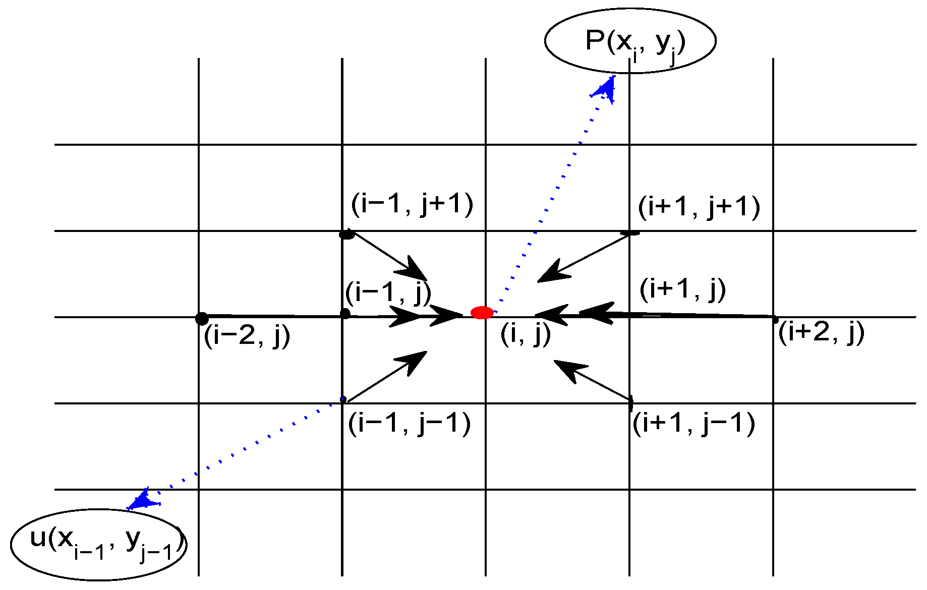
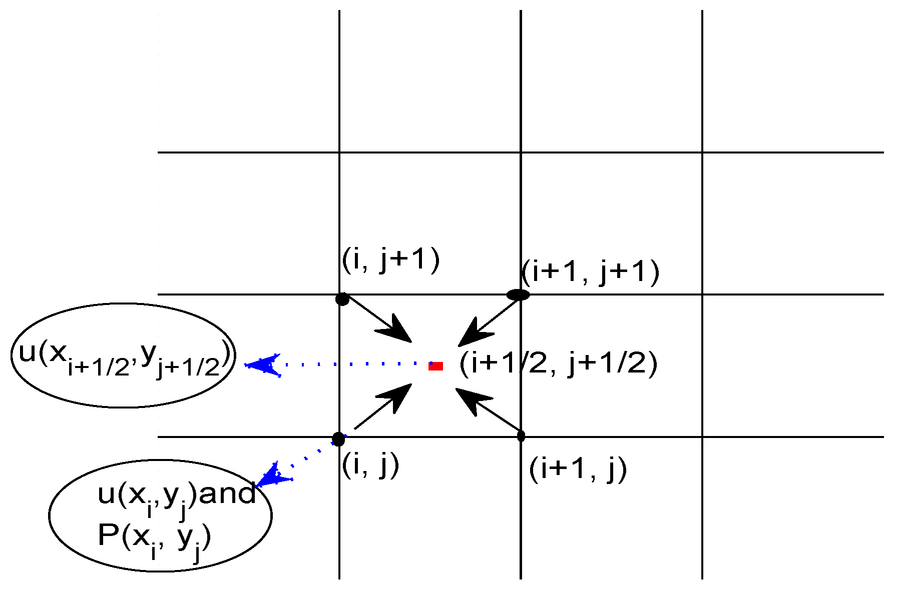
3.2.1. Local Hermite Interpolation and Refinement in the Two-Dimensional Case

For convenience, we denote:
K i , j = u x i , y j , t x = Δ u x x i , y j , t , and L i , j = u x i , y j , t y .
Let us consider Hermite bilinear interpolation functions Ψ H ( x , y , t ) on the rectangular mesh [ x i , x i + 1 ] × [ y j , y j + 1 ] Ω h , where its four vertexes are as follows:
z 1 : x i , y j , t , z 2 : x i + 1 , y j , t , z 3 : x i , y j + 1 , t , z 4 : x i + 1 , y j + 1 , t Ω h .
On the segment z 1 z 2 , let the bilinear interpolation function satisfy the following conditions:
Ψ H ( z 1 ) = u ( z 1 ) , Ψ H ( z 2 ) = u ( z 2 ) ,
( Ψ H ) x ( z 1 ) = u x ( z 1 ) , and ( Ψ H ) x ( z 2 ) = u ( z 2 ) .
Based on Reference [6], we can obtain the following Hermite interpolation polynomial:
Ψ H ( x i + 1 2 , y j , t ) = 1 2 [ u ( z 1 ) + u ( z 2 ) ] + h 8 [ u x ( z 1 ) u x ( z 2 ) ] ,
where i = 1,2 , , N 1 . The interpolation errors are:
Ψ H x i + 1 2 , y j , t u x i + 1 2 , y j , t = u x x x x ξ i , y j , t 4 ! x i + 1 2 x i 2 x i + 1 2 x i + 1 2 = h x 4 384 u x x x x ξ i , y j , t , i , j = 1 , 2 , , N 1 .
where ξ j lies between z 1 and z 2 (see Reference [6]). Thus, we obtain the following approximate computation formula for any i = 2,3 , , , N 1 , j = 1,2 , , N 1 :
u i + 1 2 , j k = 1 2 u i j k + u i + 1 , j k + h x 8 K i j K i + 1 , j .
Similarly, we have also that:
u i , j + 1 2 k = 1 2 u i j k + u i , j + 1 k + h y 8 L i j L i , j + 1 .
Therefore, for i , j = 2,3 , , N 3 , u i + 1 2 , j + 1 2 k can be approximated as follows:
u i + 1 2 , j + 1 2 k = 1 2 u i , j + 1 2 k + u i + 1 , j + 1 2 k + h 8 K i , j + 1 2 K i + 1 , j + 1 2 = 1 4 u i j k + u i , j + 1 k + h 16 L i j L i , j + 1 + L i + 1 , j L i + 1 , j + 1 + 1 4 u i + 1 , j k + u i + 1 , j + 1 k + h 16 K i j K i + 1 j + K i j + 1 K i + 1 j + 1 .
In Section 3.3, we will prove that the above refinement scheme has fourth-order accuracy in the space direction, see Theorem 5.

3.2.2. The Collocation Polynomial in the Two-Dimensional Case

Next, we use the collocation polynomial method to obtain the approximate values of K i j and L i j . For convenience, we consider the sub-domain:
[ x i 1 , x i + 1 ] × [ y j 1 , y j + 1 ] Ω , i , j = 1,2 , , N 1 ,
and denote:
ξ = x x i , η = y y j , x , y Ω h , i , j = 1 , 2 , , N 1 .
In order to get the approximation polynomial of u, we consider the polynomial space:
H 4 = s p a n 1 , ξ , η , ξ 2 , ξ η , η 2 , ξ 3 , ξ 2 η , ξ η 2 , η 3 , ξ 4 , ξ 2 η 2 , η 4 ,
and define the approximation polynomial as follows:
H ( ξ , η ) = a 0 + a 1 ξ + a 2 η + a 3 ξ 2 + a 4 ξ η + a 5 η 2 + a 6 ξ 3 + a 7 ξ 2 η + a 8 ξ η 2 + a 9 η 3 + a 10 ξ 4 + a 11 ξ 2 η 2 + a 12 η 4 .
Let:
H x m , y n = u x m , y n ; m = i 1 , i , i + 1 ; n = j 1 , j , j + 1 ; m i n j 0 ; 2 H x m , y n x 2 + 2 H x m , y n y 2 = u t x m , y n , t ,
where n = j ; m = i 1 , i , i + 1 and n = j ± 1 , m = i . Then, we can obtain the following numerical gradient approximate scheme:
K i j = 1 12 h 8 u x i + 1 , y j , t 8 u x i 1 , y j , t + u x i 2 , y j , t u x i + 2 , y j , t , i = 2 , 3 , , N 2 , j = 1 , 2 , , N 1 ;
L i j = 1 12 h 8 u x i , y j + 1 , t 8 u x i , y j 1 , t + u x i , y j 2 , t u x i , y j + 2 , t , i = 1 , 2 , , N 1 , j = 2 , 3 , , N 2 .

3.3. The Truncation Errors of the Numerical Gradient Scheme

As stated in the previous Section 2, the truncation errors of the compact difference method in Reference [5] are O ( τ 2 + h 4 ) . In fact, the above numerical gradient schemes, Equations (34) and (35), also have the same convergence order.
Theorem 4.
If u ( x , y , t ) C x 6 ( Ω ) and u ( x , y , t ) C y 6 ( Ω ) , then we have:
K i j u x i , y j , t x < O h 4 , ( i = 2 , 3 , , N 2 ; j = 1 , 2 , , N 1 ) ,
L i j u x i , y j , t y < O h 4 , j = 2 , 3 , , N 2 ; i = 1 , 2 , , N 1 .
Proof. 
According to Equation (34), we know:
K i j = 1 12 h 8 u x i + 1 , y j , t 8 u x i 1 , y j , t + u x i 2 , y j , t u x i + 2 , y j , t = 4 3 u x i + 1 , y j , t u x i 1 , y j , t 2 h 1 3 u x i 2 , y j , t u x i + 2 , y j , t 4 h .
In addition, according to the Taylor series expansion theorem, we have:
u x i , y j , t x = 4 3 u x i + 1 , y j , t u x i 1 , y j , t 2 h 1 3 u x i 2 , y j , t u x i + 2 , y j , t 4 h + O h 4
So:
u x i , y j , t x K i j = O h 4 .
Similarly, we may also prove that:
u x i , y j , t y L i j = O h 4 .
Thus the proof is completed. □
By the above theorem, we know that the accuracy of the numerical gradient schemes in Equations (34) and (35) is O ( h 4 ) in the space direction. In fact, in the intermediate points ( x i + 1 2 , y j + 1 2 , t ) , the above refinement scheme, Equation (31), also has fourth-order accuracy in space direction.
Theorem 5.
If u ( x , y , t ) C x 6 ( Ω ) and u ( x , y , t ) C y 6 ( Ω ) , then:
u x i + 1 2 , y j + 1 2 , t k u i + 1 2 , j + 1 2 k O h 4 , i , j = 2,3 , , N 3 .
Proof. 
First, by the Taylor expansion of u x i , y j , t k at ( x j + 1 2 , T ) , we have:
u x i , y j , t k = u x i + 1 2 , y j , t k h 2 u x x i + 1 2 , y j , t k + h 2 8 u x x x i + 1 2 , y j , t k h 3 48 u x x x x i + 1 2 , y j , t k + O h 4 ,
u x i + 1 , y j , t k = u x i + 1 2 , y j , t k + h 2 u x x i + 1 2 , y j , t k + h 2 8 u x x x i + 1 2 , y j , t k + h 3 48 u x x x x i + 1 2 , y j , t k + O h 4 .
Therefore:
u x i + 1 2 , y j + 1 2 , t k = 1 4 u x i , y j , t k + u x i , y j + 1 , t k + u x i + 1 , y j , t k + u x i + 1 , y j + 1 , t k h 2 8 u x x x i + 1 2 , y j + 1 2 , t k h 2 16 [ u y y x i , y j + 1 2 , t k u y y x i + 1 , y j + 1 2 , t k ] + O h 4 = 1 4 u x i , y j , t k + u x i , y j + 1 , t k + u x i + 1 , y j , t k + u x i + 1 , y j + 1 , t k h 16 y δ y u x i , y j + 1 2 , t k u x i + 1 , y j + 1 2 , t k h 8 x δ x u x i + 1 2 , y j + 1 2 , t k + O h 4 = 1 4 u i j k + u i , j + 1 k + u i + 1 , j k + u i + 1 , j + 1 k h 16 L i j L i , j + 1 + L i + 1 j L i + 1 j + 1 h 16 K i j K i + 1 , j + K i , j + 1 K i + 1 , j + 1 + O h 4 = u i + 1 2 , j + 1 2 k + O h 4 .
That is, the conclusion holds. □
In addition, to reduce the total computing time, we also consider the Richardson extrapolation on the H-OCD scheme of Equation (25) in the two-dimensional case. For convenience, we take the following initial–boundary problem as a simple example:
u t Δ u = F u x , y , t , x , y , t a , b × c , d × 0 , T , u x , c , t = u x , d , t = u a , y , t = u b , y , t = 0 , x , y a , b × c , d , 0 t T , u x , y , 0 = 0 , x , y a , b × c , d
with the smooth solution u ( x , y , t ) , where:
F u x , y , t = 1 24 3 u x , y , t t 3 1 8 4 u x , y , t x 2 t 2 .
Theorem 6.
Let u x , y , t C 8 , 6 Ω h × 0 , T be the solution of Equation (22) for the initial–boundary problem of Equation (39), and let u i j k h , τ be the numerical solution of the H-OCD scheme, Equation (25), with time step τ and spatial step h. Then:
max 1 i , j N 1 , 1 k M u x i , y j , t k 4 3 u i j 2 k h , τ 2 1 3 u j k h , τ = O τ 4 + h 4 .
Proof. 
The proof is similar to that of Theorem 3. □
In addition, the corresponding numerical experiments will be shown in Table 10.

4. Numerical Experiments

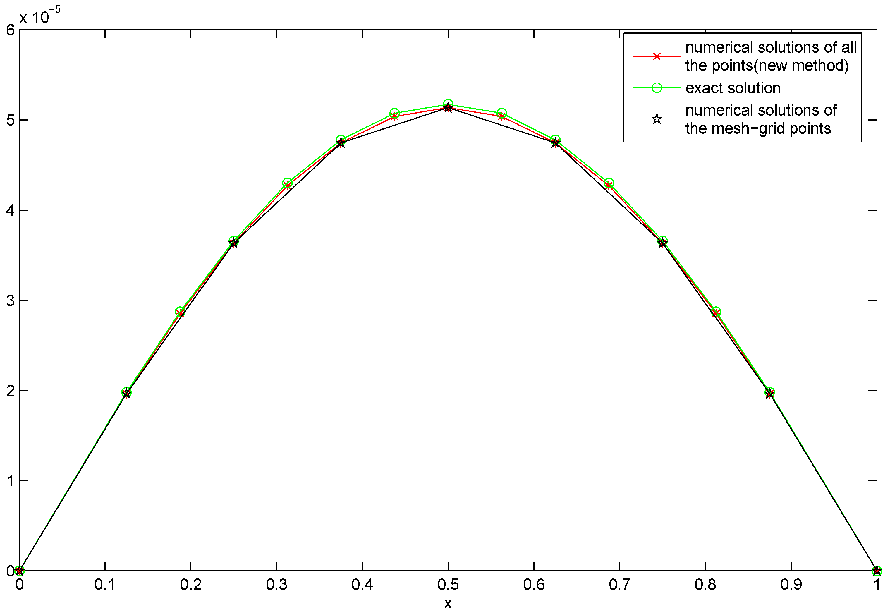
4.1. Numerical Experiments for the One-Dimensional Case

Example 1.
Let u ( x , 0 ) = sin ( π x ) , u ( 0 , t ) = u ( 1 , t ) = 0 for Equation (1) with ( x , t ) ( 0 , 1 ) × ( 0 , T ] . Then the exact solution of Equation (1) is:
u ( x , t ) = exp ( π 2 t ) sin ( π x ) .
Next, let us observe and compare the numerical solutions and computation times for the same number of points in the above two schemes.
First, we note that matrix computations are based on LAPACK, and the optimized basic linear algebra subroutines (BLAS) on the Matlab platform which speeds up matrix multiplications and the LAPACK routines themselves, according to Matlab user manual. Therefore, all the numerical experiments were performed in Matlab 2011b. In addition, for convenience, we denote R a t e ( h ) = log 2 E r r o r ( h ) E r r o r ( h 2 ) and E r r o r ( h ) = max x k = x 0 + k h , k = 0 , 1 , N { ( u ( x k , T ) u k T ) } , where u ( x k , T ) represents the exact solution and u k T is the numerical solution. Let:
E r r o r ( P ) = max x k = x 0 + k h , k = 0 , 1 , N u x ( x j , T ) P k T ) .
Table 1 lists the computational results for the mesh grid points, the intermediate points, and u x with different spatial step sizes, when time step size is fixed as τ = 1 / 100,000 . We can see that the convergence order in space can reach O ( h 4 ) which is consistent with the theoretical analysis in this article.
Figure 3 displays the errors curves with different step sizes for the mesh grid points (by the H-OCD method) and for all the points (by the new method) when T = 1 . This displays that the changes of the truncation errors in the mesh grid points and the other points are large with large h and τ . At the same time, the shape of the curves is approximately the same. That means that the points obtained through the new method are not worse than the H-OCD method.
Figure 4 shows that the numerical solution (the red line), for all the points calculated by the new method, is closer to the exact solution (the green line) when h = 1 / 8 , τ = 1 / 100 , T = 1 . That is to say, the simulation result of the red line is better than the other one. In order to make Figure 4 more clear, we choose h = 1 / 8 .
Figure 5 displays the error surface maps with different step sizes in both the spatial and time directions for the mesh grid points (by the H-OCD method) and for all the points (by the new method) when t = 1 . This display that the truncation errors in the mesh grid points and the other points are large when h and τ are large. At the same time, the shape of the curves is approximately the same. That means that the points obtained through the new method work very well too.
In addition, from Table 2, we know that the H-OCD method takes more time to compute the same number of difference points, compared to the new method. For example, if we need the numerical solutions of 255 points to simulate the real figure, we only need h = 1 / 128 . Through the method proposed in this article, we can get the numerical solutions for the 255 points.
Example 2.
For u ( x , 0 ) = exp ( x ) , u ( 0 , t ) = exp ( t ) , u ( 1 , t ) = exp ( 1 + t ) with ( x , t ) ( 0 , 1 ) × ( 0 , T ] , the exact solution of Equation (1) is:
u ( x , t ) = exp ( x + t ) .
In the following, we compare the numerical solution with the exact solution as follows (see Table 3, Table 4, Table 5 and Table 6).
From Table 3 and Table 4, we know that the numerical results are consistent with our theoretical results.
In addition, the conclusion in the space direction we get from Table 5 is the same as that from Table 2. Thus, combining with Figure 6, the advantage of the numerical gradient scheme is obvious. In Table 6, we consider the Richardson extrapolation on the H-OCD scheme of Equations (7)–(9) in the time direction. This result is consistent with Theorem 3.

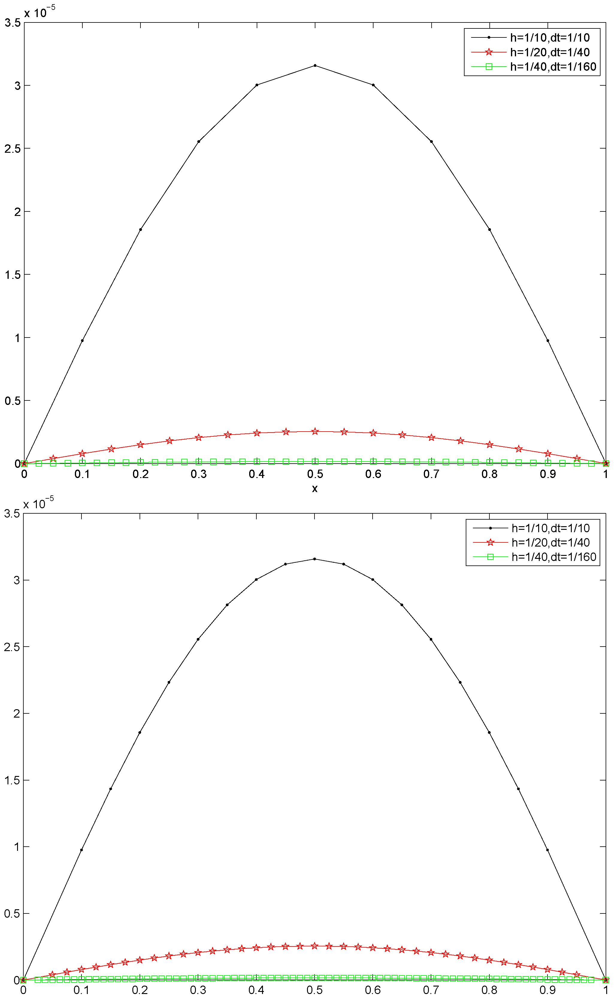
4.2. Numerical Experiments for the Two-Dimensional Case

Example 3.
When:
u x , y , 0 = sin π x sin π y , u 0 , y , t = u 1 , y , t = u x , 0 , t = u x , 1 , t = 0 ,
the exact solution of Equation (22) is:
u x , y , t = e 2 π 2 t sin π x sin π y , x , y , t Ω × 0 , T .
Next, let us observe and compare the numerical solutions from the different methods.
Table 7 lists the computational results for the mesh grid points and intermediate points with different spatial step sizes, when the time step size is fixed as τ = 1 / 100,000 . We can see that the convergence orders in space can reach O ( h 4 ) which is consistent with the theoretical analysis (see Theorems 4 and 5) in this article. In addition, from Table 8, we see also that the numerical gradient scheme has the same convergence order O ( τ 2 + h 4 ) as the H-OCD method when the time and space step sizes are the same.
In addition, Table 9 and Figure 6 also show similar results to those of Table 5 and Figure 3 and Figure 4, respectively. Table 10 lists the computational results for the Richardson extrapolation scheme. These results show that the convergence order in time direction can reach O ( τ 4 ) , which is consistent with the theoretical analysis (see Theorem 6).
For this two-dimension problem, we have obtained similar experimental results as the previous one-dimension problem, which shows that this method is effective.

5. Conclusions

Recently, many people have devoted themselves to the development of numerical approximations of heat equation problems. By numerical comparisons, we know that the high-order compact difference scheme (H-OCD) of Reference [5] is better than the traditional numerical schemes. In this article, we further improve this method to a new numerical gradient scheme. Moreover, our theoretical analysis and numerical experiments show that this numerical gradient scheme has the same convergence order as the H-OCD in Reference [5]. We hope that this is a useful supplement to the existing results. The results also provide potential for several applications for example those in References [11,12,13,14].
In addition, many new methods have recently emerged for solving differential equations such as the Lie algebra method [15,16]. Absorbing or drawing on the advantages of these methods to obtain better results is a problem worthy of further study.

Author Contributions

Conceptualization, E.-J.Z.; Funding acquisition, H.-B.L.; Date, X.-M.G.; Supervision, H.-B.L. and X.-M.G.; Writing-original draft, M.-Y.S. and H.-B.L.; and Writing-review and editing, H.-B.L. and X.-M.G.

Funding

This work was financially supported by the National Natural Science Foundation of China (11271001, 11101071), and the Fundamental Research Funds for the Central Universities(ZYGX2016J138).

Acknowledgments

The authors would like to thank reviewers and editors for providing us some good suggestions and help.

Conflicts of Interest

The authors declare no conflict of interest.

References

  1. Hu, J.W.; Tang, H.M. Numerical Methods of Differential Equations; Science Press: Berlin, Germany, 2007. [Google Scholar]
  2. Morton, K.W. Numerical Solutions of Partial Differential Equations, 2nd ed.; Posts and Telecom Press: Beijing, China, 2006. [Google Scholar]
  3. Sun, Z.Z. Compact Difference Schemes for Heat Equations with the Neumann Boundary Conditions. Numer. Method Partial Differ. Equ. 2009, 25, 1320–1341. [Google Scholar] [CrossRef]
  4. Zhang, W.S. Finite Difference Methods for Partial Difference Equations in Science Computation; Higher Education Press: Beijing, China, 2006. [Google Scholar]
  5. Sun, Z.Z.; Zhang, Z.B. A Linearized Compact Difference Schemes for a Class of Nonlinear Delay Partial Differential Equations. Appl. Math. Model. 2013, 37, 742–752. [Google Scholar] [CrossRef]
  6. Timothy, S. Numerical Analysis; Posts and Telecom Press: Beijing, China, 2010. [Google Scholar]
  7. Liao, H.L.; Sun, Z.Z.; Shi, H.S. Error Estimate of Fourth-order Compact Scheme for Linear Schromdinger Equations. SIAM Numer. Anal. 2010, 47, 4381–4401. [Google Scholar] [CrossRef]
  8. Richardson, L.F. The approximate arithmetical solution by finite differences of physical problems including differential equations, with an application to the stresses in a masonry dam. Philos. Trans. R. Soc. A 1911, 210, 307–357. [Google Scholar] [CrossRef]
  9. Liao, H.L.; Sun, Z.Z. Maxmum Norm Error Bounds of ADI and Compact ADI methods for Solving Parabolic Equations. Numer. Method Partial Differ. Equ. 2010, 26, 37–60. [Google Scholar] [CrossRef]
  10. Sun, Z.Z. Numerical Methods of Partial Differential Equations; Science Press: Berlin, Germany, 2012. [Google Scholar]
  11. Ikota, R.E. Yanagida. Stability of stationary interfaces of binary-tree type. Calc. Var. Partial Differ. Equ. 2004, 22, 375–389. [Google Scholar] [CrossRef]
  12. Dassios, I. Stability of basic steady states of networks in bounded domains. Comput. Math. Appl. 2015, 70, 2177–2196. [Google Scholar] [CrossRef]
  13. Dassios, I. Stability of Bounded Dynamical Networks with Symmetry. Symmetry 2018, 10, 121. [Google Scholar] [CrossRef]
  14. Xiaofeng, R.; Wei, J. A Double Bubble in a Ternary System with Inhibitory Long Range Interaction. Arch. Ration. Mech. Anal. 2013, 208, 201–253. [Google Scholar]
  15. Shang, Y. A Lie algebra approach to susceptible-infected-susceptible epidemics. Electron. J. Differ. Equ. 2012, 2012, 147–154. [Google Scholar]
  16. Shang, Y. Analytical Solution for an In-host Viral Infection Model with Time-inhomogeneous Rates. Acta Phys. Pol. Ser. B 2015, 46, 1567–1577. [Google Scholar] [CrossRef]
Figure 1. The relationships between u ( x i + 1 2 , y j + 1 2 ) , and the surrounding points u ( x i , y j ) and partial derivatives P ( x i , y j ) .
Mathematics 07 00093 g001
Figure 2. The relationships between P ( x i , y j ) and the surrounding points u ( x i , y j ) .
Mathematics 07 00093 g002
Figure 3. (Top) The error curves of the mesh grid points in the high-order compact difference (H-OCD) method, when T = 1 ; (Bottom) The error curves of all the points in the new method, when T = 1 .
Mathematics 07 00093 g003
Figure 4. The numerical solutions and the exact solution for all the points in the new method and for the mesh grid points in the H-OCD method, when h = 1 / 8 , τ = 1 / 100 , t = 1 .
Mathematics 07 00093 g004
Figure 5. (Top) The error surface map of the compact difference scheme for the mesh grid points; (Bottom) The error surface map of the numerical gradient scheme for the intermediate points.
Mathematics 07 00093 g005
Figure 6. Curves of the numerical solutions and the exact solution for Example 3 when h = 1 / 20 , τ = 1 / 400 , T = 1 .
Mathematics 07 00093 g006
Table 1. Errors and rate for calculations of the intermediate points and numerical gradients P in space direction, with τ = 1 / 100,000 .
hMesh Grid PointsRateIntermediate PointsRateP (i.e., u x )Rate
ErrorErrorError
1/4 8.3491 × 10 7 4.0355 5.4790 × 10 7 3.5729 3.7721 × 10 6 3.7762
1/8 5.0915 × 10 8 4.0073 4.6043 × 10 8 3.9694 2.5732 × 10 7 3.9370
1/16 3.1660 × 10 9 4.0045 2.9394 × 10 9 3.9952 1.7976 × 10 8 3.9823
1/32 1.9725 × 10 10 4.0466 1.8433 × 10 10 4.0474 1.1374 × 10 9 3.9715
1/64 1.1936 × 10 11 - 1.1148 × 10 11 - 7.2504 × 10 11 -
Table 2. Errors of the numerical solutions in the mesh grid points (H-OCD method), and in all the points (numerical gradient scheme), and the total time to calculate the solutions when τ = h 2 , T = 1 , h = 1 / ( n 1 ) .
Grid Node NumberH-OCD MethodTimeNumerical Gradient SchemeTime
ErrorError
N = 15 6.0041 × 10 8 0.1544 9.5518 × 10 7 0.0312
N = 31 3.7541 × 10 9 0.5725 6.0041 × 10 8 0.1560
N = 63 2.3464 × 10 10 2.5389 3.7623 × 10 9 0.5839
N = 127 1.4665 × 10 11 11.505 2.3536 × 10 10 2.7233
N = 255 9.1633 × 10 13 142.64 1.4713 × 10 11 12.8879
Table 3. Errors and rates of the H-OCD scheme, Equations (7)–(9), the intermediate points (new method), and the numerical gradient P j in the spatial direction, with τ = 1 / 100,000 .
hMesh-Grid PointsRateIntermediate PointsRateP (i.e., u x )Rate
ErrorErrorError
1/4 8.4064 × 10 6 3.9974 2.9136 × 10 4 3.8091 6.8324 × 10 3 2.7543
1/8 5.2636 × 10 7 3.9895 2.0787 × 10 5 3.9099 1.1027 × 10 3 2.8763
1/16 3.3138 × 10 8 3.9993 1.3828 × 10 6 3.9564 1.3792 × 10 4 2.9379
1/32 2.0721 × 10 9 4.0472 8.9081 × 10 8 3.9787 1.7998 × 10 5 2.9689
1/64 1.2534 × 10 10 - 5.6505 × 10 9 - 2.2987 × 10 6 -
Table 4. Errors and rates of the H-OCD scheme, Equations (7)–(9), the intermediate points (new method), and the numerical gradient P j in the time direction, with h = 1 / 10,000 .
τ Compact DifferenceRateIntermediate PointsRateP (i.e., u x )Rate
ErrorErrorError
1/10 4.3449 × 10 4 1.9988 4.3449 × 10 4 1.9988 2.0491 × 10 3 1.9769
1/20 1.0871 × 10 4 1.9998 1.0871 × 10 4 1.9998 5.2055 × 10 4 1.9887
1/40 2.7183 × 10 5 1.9999 2.7183 × 10 5 1.9999 1.3116 × 10 4 1.9945
1/80 6.7960 × 10 6 2.0005 6.7960 × 10 6 2.0005 3.2914 × 10 5 1.9987
1/160 1.6984 × 10 6 2.0053 1.6984 × 10 6 2.0053 8.2362 × 10 6 2.0053
1/320 4.2303 × 10 7 2.0246 4.2303 × 10 7 2.0246 2.0515 × 10 6 2.0259
1/640 1.0397 × 10 7 - 1.0397 × 10 7 - 5.0375 × 10 7 -
Table 5. Errors of the numerical solutions for the mesh grid points and for all points in the new method, and the time to get these solutions when τ = h 2 , t = 1 , h = 1 / ( n 1 ) .
Grid Node NumberH-OCD MethodTimeNumerical Gradient SchemeTime
ErrorError
N = 15 6.2975 × 10 7 0.1248 1.3540 × 10 5 0.0406
N = 31 3.9376 × 10 8 0.5725 1.1199 × 10 6 0.1265
N = 63 2.4630 × 10 9 3.1590 8.0259 × 10 8 0.5959
N = 127 1.5453 × 10 10 20.117 5.3654 × 10 9 3.1844
N = 255 1.2050 × 10 11 128.44 3.4669 × 10 10 21.542
Table 6. Errors and rates for all points in the new method for Examples 1 and 2 when τ = h , T = 1 .
τ = h Example 1 error ( h , τ ) error ( h / 2 , τ / 2 ) Example 2 error ( h , τ ) error ( h / 2 , τ / 2 )
ErrorError
1/8 5.5147 × 10 6 14.2567 2.0369 × 10 5 14.9661
1/16 3.8682 × 10 7 15.6251 1.3610 × 10 6 15.4867
1/32 2.4756 × 10 8 15.9066 8.7881 × 10 8 15.7438
1/64 1.5563 × 10 9 15.9741 5.5819 × 10 9 15.8711
1/128 9.7429 × 10 11 15.9934 3.5170 × 10 10 15.9209
1/256 6.0918 × 10 12 - 2.2091 × 10 11 -
Table 7. Errors and rates for intermediate points and numerical gradients P in spatial direction with τ = 1 / 100,000 .
hH-OCD Mesh-Grid PointsRateIntermediate Points (New Method)Rate
ErrorError
1/4 5.3017 × 10 11 3.9403--
1/8 3.4536 × 10 12 3.9878 4.6576 × 10 12 3.9629
1/16 2.1769 × 10 13 3.9805 2.9869 × 10 13 3.9791
1/32 1.3791 × 10 14 - 1.8939 × 10 14 -
Table 8. Errors and rates of all points (new method) for Example 3 when τ = h 2 , h = 1 / n 1 , T = 1 .
NH-OCD Method error ( h , τ ) error ( h / 2 , τ / 2 ) Numerical Gradient error ( h , τ ) error ( h / 2 , τ / 2 )
ErrorError
N = 5 1.6485 × 10 9 9.7908 1.8257 × 10 9 11.0802
N = 10 1.6838 × 10 10 15.6079 1.6477 × 10 10 15.3196
N = 20 1.0788 × 10 11 15.9751 1.0755 × 10 11 15.9015
N = 40 6.7530 × 10 13 - 6.7638 × 10 13 -
Table 9. A comparison of the computation time between the H-OCD method and the numerical gradient scheme.
Grid NumberH-OCD Method Grid NumberNumerical Gradient
ErrorTimeErrorTime
n = 16 1.6485 × 10 9 0.0374n = 17 1.8257 × 10 9 0.0421
n = 81 1.6838 × 10 10 0.4563n = 117 1.6838 × 10 10 0.5756
n = 224 3.3602 × 10 11 2.8782n = 433 3.4081 × 10 11 2.8860
n = 361 1.0788 × 10 11 9.0527n = 745 1.0788 × 10 11 10.8556
n = 624 4.4056 × 10 12 25.2347n = 1233 4.4370 × 10 12 26.8556
n = 899 2.1338 × 10 12 63.2506n = 1783 2.1347 × 10 12 66.8199
n = 1599 6.7530 × 10 13 422.8602n = 3183 6.7638 × 10 13 424.2073
Table 10. The convergence order for the Richardson extrapolation scheme of Example 3 when τ = h / 20 , T = 1 .
hH-OCD Method error ( h , τ ) error ( h / 2 , τ / 2 ) Numerical Gradient error ( h , τ ) error ( h / 2 , τ / 2 )
ErrorError
h = 1/5 2.1070 × 10 11 14.1419 3.2895 × 10 11 16.4508
h = 1/10 1.4899 × 10 12 15.9254 1.9996 × 10 12 15.7474
h = 1/20 9.3555 × 10 14 15.9822 1.2698 × 10 13 15.9392
h = 1/40 5.8537 × 10 15 15.9955 7.9665 × 10 15 15.9848
h = 1/40 3.6596 × 10 16 - 4.9838 × 10 16 -

